DESY 98–116
TPR–98–23
HUB–EP–98/49
September 1998
Composite operators in lattice QCD: nonperturbative renormalization

Abstract

We investigate the nonperturbative renormalization of composite operators in lattice QCD restricting ourselves to operators that are bilinear in the quark fields. These include operators which are relevant to the calculation of moments of hadronic structure functions. The computations are based on Monte Carlo simulations using quenched Wilson fermions.

1 INTRODUCTION

Lattice investigations of hadronic structure require the calculation of hadronic matrix elements of composite operators. In general, one has to convert the bare lattice operators into renormalized continuum operators by multiplication with the appropriate renormalization coefficient $Z$. The accuracy of perturbative calculations of these $Z$ factors remains uncertain, even if tadpole improvement [1] is used, as more than a one-loop computation is rarely available. Therefore a nonperturbative calculation by Monte Carlo simulations appears to be an attractive alternative [2].

We have performed such a computation for operators that determine moments of hadronic structure functions. Computing the $Z$ factors for a rather large range of renormalization scales we try to find out at which scales (if at all) perturbative behavior sets in such that the multiplication with perturbative Wilson coefficients makes sense. For further details and results see Ref. [3].

We use standard Wilson fermions in the quenched approximation. At $\beta=6.0$ ($\beta=6.2$) we work on a $16^{3}\times 32$ ($24^{3}\times 48$) lattice. For both $\beta$’s we have studied three values of the hopping parameter $\kappa$.

In this talk, we shall concentrate on one particular example, namely the operator

$${\cal O}=\bar{q}\left(\gamma_{4}\mbox{ \parbox[b]{0.0pt}{$D$}\raisebox{7.3194pt}{$\leftrightarrow$}${}_{\!4}$}-\frac{1}{3}\sum_{i=1}^{3}\gamma_{i}\mbox{ \parbox[b]{0.0pt}{$D$}\raisebox{7.3194pt}{$\leftrightarrow$}${}_{\!i}$}\right)q\,,$$ (1)

(${\cal O}_{v_{2,b}}$ in the notation of Ref. [3]) whose hadronic matrix elements are proportional to the momentum fraction $\langle x\rangle$ carried by the quarks. Working with Wilson fermions it is straightforward to write down a lattice version of the above operator. One simply replaces the continuum covariant derivative by its lattice analogue.

2 THE METHOD

We follow the procedure proposed by Martinelli et al. [2]. It applies the definitions used in (continuum) perturbation theory to vertex functions calculated by Monte Carlo simulations on the lattice. To be more specific, we calculate the quark-quark Green function (a matrix in color and Dirac space) with one insertion of the operator ${\cal O}$ at momentum zero in the Landau gauge. Amputating the external quark legs we obtain the vertex function $\Gamma(p)$ as a function of the quark momentum $p$. Defining the renormalized vertex function by $\Gamma_{\mathrm{R}}(p)=Z_{q}^{-1}Z\Gamma(p)$ we fix the renormalization constant $Z$ by imposing the condition

$$\mbox{\small$\frac{1}{12}$}{\rm tr}\left(\Gamma_{\mbox{\scriptsize R}}(p)\Gamma_{\mbox{\scriptsize Born}}(p)^{-1}\right)=1$$ (2)

at $p^{2}=\mu^{2}$, where $\mu$ is the renormalization scale. So we calculate $Z$ from

$$Z_{q}^{-1}Z\mbox{\small$\frac{1}{12}$}{\rm tr}\left(\Gamma(p)\Gamma_{\mbox{\scriptsize Born}}(p)^{-1}\right)=1$$ (3)

with $p^{2}=\mu^{2}$. Here $\Gamma_{\mbox{\scriptsize Born}}(p)$ is the Born term in the vertex function of ${\cal O}$ computed on the lattice, and $Z_{q}$ denotes the quark field renormalization constant. The latter is calculated from the quark propagator $S(p)$:

$$Z_{q}(p)=\frac{{\rm tr}\left(-{\rm i}\sum_{\lambda}\gamma_{\lambda}\sin(ap_{\lambda})aS^{-1}(p)\right)}{12\sum_{\lambda}\sin^{2}(ap_{\lambda})}\,,$$ (4)

again at $p^{2}=\mu^{2}$.

3 PERTURBATIVE INPUT

Eq. (2) defines a renormalization scheme of the momentum subtraction type, which we call MOM scheme. In order to convert our results into the more popular $\overline{\mbox{MS}}$ scheme we have to perform a finite renormalization. The corresponding renormalization constant $Z^{\overline{\mathrm{M}S}}_{\mathrm{M}OM}$ is computed in continuum perturbation theory using dimensional regularization.

Neglecting quark masses we obtain in the Landau gauge

$$\begin{array}[]{l}\displaystyle Z^{\overline{\mathrm{M}S}}_{\mathrm{M}OM}=1+\frac{g^{2}}{16\pi^{2}}C_{F}\Bigg{[}-\frac{31}{9}\\ \displaystyle\quad{}-\frac{\left(p_{4}^{2}-\mbox{\small$\frac{1}{3}$}(p_{1}^{2}+p_{2}^{2}+p_{3}^{2})\right)^{2}}{3p^{2}\left(p_{4}^{2}+\mbox{\small$\frac{1}{9}$}(p_{1}^{2}+p_{2}^{2}+p_{3}^{2})\right)}\Bigg{]}+O(g^{4})\,,\end{array}$$ (5)

where $C_{F}=4/3$ for the gauge group SU(3). Because of the noncovariance of the condition (2), $Z^{\overline{\mathrm{M}S}}_{\mathrm{M}OM}$ depends on the direction of the momentum $p$.

For the scale dependence, the renormalization group predicts (at fixed bare parameters)

$$\begin{array}[]{l}\displaystyle R(\mu,\mu_{0}):=\frac{Z(\mu)}{Z(\mu_{0})}\\ \displaystyle\quad{}=\exp\left\{-\int_{\bar{g}(\mu_{0}^{2})}^{\bar{g}(\mu^{2})}\mathrm{d}g\frac{\gamma(g)}{\beta(g)}\right\}\end{array}$$ (6)

in terms of the running coupling $\bar{g}(\mu^{2})$, the $\beta$-function $\beta(g)$, and the anomalous dimension $\gamma(g)$. An analogous formula describes the $\beta$ dependence at fixed renormalized quantities.

4 RESULTS

Calculating the necessary two- and three-point functions with the help of momentum sources [3, 4, 5] we achieve small statistical errors with a moderate number of configurations. After extrapolating to the chiral limit (linearly in $1/\kappa$) we multiply by $Z^{\overline{\mathrm{M}S}}_{\mathrm{M}OM}$.

For the presentation of our results we convert lattice units to physical units using $a^{-2}=3.8$ GeV² ($\beta=6.0$) and $a^{-2}=7.0$ GeV² ($\beta=6.2$) as determined from the string tension [6]. The $\Lambda$ parameter is taken to be $\Lambda_{\overline{\mathrm{MS}}}=230$ MeV.

The scale dependence of our $Z$’s should be described by the renormalization group factor $R$ (see (6)). Hence we divide our numerical results by this expression (evaluated in two-loop approximation with $\mu_{0}^{2}=4$ GeV²) and define $Z_{\mathrm{RGI}}=Z/R$. For $Z_{\mathrm{RGI}}$ we hope to obtain a $\mu$ independent answer, at least in a reasonable window of $\mu$ values. There $\mu^{2}$ would be large enough to allow for perturbative scaling behavior. On the other hand, $\mu^{2}$ should be small enough to avoid strong cut-off effects.

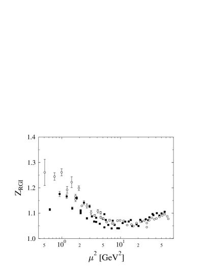
Figure 1: $Z_{\mathrm{RGI}}$ for the operator ${\cal O}$ (Eq. (1)). The open circles (filled squares) represent the data for $\beta=6.2$ ($\beta=6.0$). The $\beta=6.2$ data have been rescaled perturbatively to $\beta=6.0$.

In Fig. 1 we plot $Z_{\mathrm{RGI}}$ versus the renormalization scale $\mu^{2}$ for our operator ${\cal O}$. The errors are purely statistical. A “flat” region seems to start at $\mu^{2}\approx 5$ GeV². Note that the $\beta=6.0$ data and the (perturbatively rescaled) $\beta=6.2$ data agree except for the lowest values of $\mu^{2}$. This indicates that the observed $\mu$ dependence is physical. For other operators, the results look qualitatively similar, although in most cases a window starts only at $\mu^{2}\approx 10$ GeV², where it is hard to believe that cut-off effects are negligible.

In Fig. 2 we compare the nonperturbative values for $Z$ in the $\overline{\mathrm{MS}}$ scheme with (tadpole improved) one-loop lattice perturbation theory. We plot the results for all operators with derivatives studied in Ref. [3] at $\mu^{2}=a^{-2}$ versus $n_{D}$, the number of derivatives. One-loop perturbation theory underestimates the increase of $Z$ with $n_{D}$. Tadpole improvement works in the right direction for $n_{D}>1$ without being quantitatively satisfactory. However, the differences between the three methods decrease as $\beta$ (and $\mu^{2}$) becomes larger.

Figure 2: Collection of $Z$’s in the $\overline{\mathrm{MS}}$ scheme versus the number of derivatives in the operators. The squares represent the nonperturbative results, the diamonds (filled circles) correspond to the values obtained in lattice perturbation theory (with tadpole improvement). The $\beta=6.0$ ($\beta=6.2$) data are displaced to the left (right).

5 SUMMARY

In summary, we have performed a comprehensive study of nonperturbative renormalization for various operators in the framework of lattice QCD. Twist-2 operators appearing in unpolarized (polarized) deep-inelastic scattering have been studied for all spins $\leq 4$ ($\leq 3$) [3]. The scale dependence of $Z$ for the operator considered in this talk agrees with perturbative expectations to a good approximation already for moderate values of $\mu^{2}$. However, most of the other operators containing covariant derivatives seem to approach perturbative scaling only for rather large values of the renormalization scale where cut-off effects might contaminate the results. The behavior at smaller $\mu^{2}$ could be nonperturbative physics, but at present we cannot exclude the possibility that it is faked, e.g., by finite-size effects. In any case, it might not always be sensible to combine these nonperturbative $Z$’s with perturbative Wilson coefficients using a scale of, say, $\mu^{2}=4$ GeV². We have therefore started a nonperturbative calculation of the Wilson coefficients. First results are reported in Ref. [7].

References

- [1] G.P. Lepage and P.B. Mackenzie, Phys. Rev. D48 (1993) 2250.
- [2] G. Martinelli et al., Nucl. Phys. B445 (1995) 81.
- [3] M. Göckeler et al., Preprint DESY 98-097 (hep-lat/9807044).
- [4] M. Göckeler et al., Nucl. Phys. B (Proc. Suppl.) 63 (1998) 868.
- [5] H. Oelrich, Thesis (Hamburg, 1998).
- [6] M. Göckeler et al., Phys. Rev. D57 (1998) 5562.
- [7] D. Petters, these proceedings.