BI-TP 98/23 
August 1998

The Calculation of Critical Amplitudes
in SU(2) Lattice Gauge Theory

J. Engels and T. Scheideler

Fakultät für Physik, Universität Bielefeld, D-33615 Bielefeld, Germany

Abstract

We calculate the critical amplitudes of the Polyakov loop and its susceptibility at the deconfinement transition of (3+1) dimensional $SU(2)$ gauge theory. To this end we study the corrections due to irrelevant exponents in the scaling functions. As a guiding line for determining the critical amplitudes we use envelope equations which we derive from the finite size scaling formulae of the observables. We have produced new high precision data on $N_{\sigma}^{3}\times 4$ lattices for $N_{\sigma}=12,18,26$ and 36. With these data we find different corrections to the asymptotic scaling behaviour above and below the transition. Our result for the universal ratio of the susceptibility amplitudes is $C_{+}/C_{-}=4.72(11)$ and thus in excellent agreement with a recent measurement for the $3d$ Ising model.

1 Introduction

The calculation of critical exponents at the critical point of second order transitions with Monte Carlo methods is by now standard. To this end one has to simulate the theory under consideration in different volumes in the immediate neighbourhood of the transition point. The behaviour of thermodynamic quantities in the thermodynamic limit is then inferred from extrapolation formulae which are derived from finite size scaling (FSS) theory. This allows in principle a classification of the underlying theory, because the critical exponents are universal for all models belonging to the same universality class. Yet the differences between the exponents of different classes may be rather small. Further tests on universality should then be performed. Indeed, since members of the same class are also sharing various scaling functions it can be shown that certain critical point amplitude combinations are universal as well [1]. Their calculation using finite volume simulations is, however, far more demanding, than in the case of the critical indices. The reason for this is that the amplitudes have to be taken from the $tL^{1/\nu}\rightarrow\infty$ limit of the scaling functions, where $t~{}$is the reduced temperature and $L$ is the characteristic length scale, $L=V^{1/d}$, i.e. essentially from very large volumes.

Recently Caselle and Hasenbusch [2] were able to show that it is possible to obtain Monte Carlo estimates for critical point amplitude ratios in the $3d$ Ising model with a precision comparable to those of other approaches [3]$-$[10]. In the more complex $SU(2)$ gauge theory in (3+1) dimensions, which is a member of the same universality class, this has been a dream for quite some time. An early attempt [11] to deduce information on amplitudes from Monte Carlo data in $SU(2)$ led to the conclusion, that the existing data were still inadequate for meaningful comparisons to results from analytic calculations. As we shall see later, both the quality of the data and the method of determination of the amplitudes are of great importance for the success of the project. There are other difficulties : the critical point has to be known with high accuracy, because a shift changes the estimates of the scaling functions. In the $3d$ Ising model the critical point has been determined with extreme precision, and simulations on really large lattices - up to $L=120$ in [2] - have been performed. Such lattice sizes are still out of reach for $SU(2)$ calculations.

In view of this situation we have chosen a different method from Caselle and Hasenbusch. We proceed in the following way. In section 2 we describe how one can control the approach to the asymptotic scaling form. For this purpose we consider the envelope function to the family of curves, which one obtains for different volumes. In the following section we present our data. Section 4 contains the analysis. Here, we first ascertain again the location of the critical point [12] with the new data, then we study the scaled observables and examine the corrections to the scaling functions. The critical amplitudes are finally derived from the estimates of the corrected scaling functions. We close with a summary and the conclusions.

2 The Approach to the Asymptotic Scaling Form

2.1 Critical point amplitudes

To stay as general as possible we use in this section the notation for magnetic systems. We define the reduced temperature $t$ as

$$t={T-T_{c}\over T_{c}},$$ (2.1)

where $T$ ist the temperature and $T_{c}$ the critical temperature. In the thermodynamic limit the correlation length $\xi$ diverges at a second order transition as

$$\xi=f_{\pm}|t|^{-\nu}.$$ (2.2)

Here the index of the critical amplitude $f$ refers to the symmetric (+) or to the broken phase ($-$) and coincides for magnetic systems with the sign of $t$. The magnetization or order parameter ${\langle M\rangle}$ and the magnetic susceptibility $\chi$ behave for zero external magnetic field $H$ close to the critical point as follows

$${\langle M\rangle}=B(-t)^{\beta}~{}~{}{\rm for~{}}t<0~{},$$ (2.3)

and

$$\chi=C_{\pm}|t|^{-\gamma}.$$ (2.4)

Though the amplitudes $C_{+}$ and $C_{-}$ are not universal, their ratio is. The same is true for $f_{+}$ and $f_{-}$. More universal amplitude ratios are obtained by making use of the hyperscaling relations among the critical exponents.

2.2 Finite size scaling

The approach to the just mentioned asymptotic scaling forms of the thermodynamic quantities is described by finite size scaling equations. In particular, it can be shown [13] using renormalization group theory that the singular part of the free energy density has the form

$$f_{s}(t,H,L)=L^{-d}Q_{f_{s}}(g_{T}L^{1/\nu},g_{H}L^{{(\beta+\gamma)}/\nu},g_{i}L^{\lambda_{i}})~{}.$$ (2.5)

The scaling function $Q_{f_{s}}$ depends on the temperature $T$ and the external field strength $H$ in terms of a thermal and a magnetic scaling field

$$g_{T}=c_{T}t+O(tH,t^{2})~{},$$ (2.6)

$$g_{H}=c_{H}H+O(tH,H^{2})~{},$$ (2.7)

and possibly further irrelevant scaling fields $g_{i}$ with negative exponents $\lambda_{i}$. All scaling fields are independent of $L$.

The order parameter ${\langle M\rangle}$, the susceptibility $\chi$ and the normalized fourth cumulant $g_{r}$ of the magnetization

$$g_{r}={{\langle M^{4}\rangle}\over{{\langle M^{2}\rangle}}^{2}}-3~{},$$ (2.8)

are obtained from $f_{s}$ by taking derivatives with respect to $H$ at $H=0$. The general form of the scaling relations derived in this way for an observable $O$ is

$$O(t,L)=L^{\rho/\nu}\cdot{\bar{Q}}(g_{T}L^{1/{\nu}},g_{i}L^{\lambda_{i}})~{}.$$ (2.9)

Here $O$ is ${\langle M\rangle},\chi$ or $g_{r}$ with $\rho=-\beta,\gamma~{}{\rm and}~{}0$, respectively. Taking into account only the largest irrelevant exponent $\lambda_{1}=-\omega$ and inserting the expansion 2.6 into $\bar{Q}$ we arrive for small $|t|$ at

$$O(t,L)=L^{\rho/\nu}\cdot Q(tL^{1/{\nu}},L^{-\omega})~{}.$$ (2.10)

2.3 Control of approach to the thermodynamic limit

The functions $O(t,L)$ for a specific observable build a family of curves, parametrized by $L$. For increasing $L$ these functions are supposed to approach the limiting form

$$O_{\infty}(t)=a_{0}|t|^{-\rho}{\rm~{}~{}for~{}~{}}|t|\rightarrow 0.$$ (2.11)

An inspection of such an ensemble of curves from Monte Carlo measurements on different volumes suggests that one calculate the envelope function to the family of curves. An example of this is the magnetization in $SU(2)$ shown in Fig. 1.

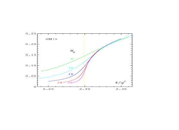
Figure 1: The modulus of the Polyakov loop ${\langle|M|\rangle}$ as function of $4/g^{2}$ on $N_{\sigma}^{3}\times 4$ lattices. The dashed line shows the location of the critical point.

At least the leading term in $t$ of this function should coincide with the limiting form eq. 2.11. The amplitude could then be determined from the envelope function.

We derive the envelope function from the FSS formula 2.10

$$F_{e}=OL^{-\rho/\nu}-Q=0,$$ (2.12)

by solving the equation

$${\partial F_{e}\over\partial L}=0$$ (2.13)

for $L=L(t)$ and insertion into eq. 2.12. Here $L(t)$ defines the matching point $t$, where the envelope function touches the curve with parameter $L(t)$. The scaling function $Q$ depends only on the scaled reduced temperature $x$ and the correction-to-scaling variable $y$

$$x=tL^{1/\nu},~{}~{}y=L^{-\omega}~{}.$$ (2.14)

Eq. 2.13 can then be written as

$$0=\rho Q+x{\partial Q\over\partial x}-\omega\nu y{\partial Q\over\partial y}~{}.$$ (2.15)

In the following we assume a linear dependence of $Q$ on $y$

$$Q(x,y)=Q_{0}(x)+yQ_{1}(x)~{},$$ (2.16)

which is certainly justified for large $L$. We will check our data for this point. Inserting the last equation into eq. 2.15 leads to

$$0=\rho Q_{0}(x)+xQ_{0}^{\prime}(x)+y\left[(\rho-\omega\nu)Q_{1}(x)+xQ_{1}^{\prime}(x)\right]~{}.$$ (2.17)

The last equation can be solved in a first approximation for $y=0$ by determining $x_{0}$ from

$$0=\rho Q_{0}(x_{0})+x_{0}Q_{0}^{\prime}(x_{0})~{},$$ (2.18)

which corresponds to the approximate matching point

$$L_{0}=\left({x_{0}\over t}\right)^{\nu}.$$ (2.19)

The next approximation $L_{1}$ is obtained from the ansatz

$$L_{1}^{1/\nu}={x_{0}\over t}(1+\epsilon(t))={x_{1}\over t}~{}~{},$$ (2.20)

with the result

$$\epsilon(t)={(t/x_{0})^{\omega\nu}\tilde{Q}_{1}\over\rho(\rho+1)Q_{0}-x_{0}^{2}Q_{0}^{\prime\prime}-(t/x_{0})^{\omega\nu}(\omega\nu\tilde{Q}_{1}+x_{0}\tilde{Q}_{1}^{\prime})}~{}~{},$$ (2.21)

where

$$\tilde{Q}_{1}=(\rho-\omega\nu)Q_{1}+x_{0}Q_{1}^{\prime}~{}~{},$$ (2.22)

and all $Q$ have to be taken at $x=x_{0}$.

Inserting $L_{1}(t)$ into eq. 2.12 gives the envelope function

$$O_{e}=({t\over x_{0}})^{-\rho}\left\{Q_{0}(x_{0})+({t\over x_{0}})^{\omega\nu}Q_{1}(x_{0})+O(|t|^{2\omega\nu})\right\}~{}.$$ (2.23)

The sign of $t$ and $x_{0}$ are here the same, the envelope function exists only on that side of the transition, where a solution $x_{0}$ to eq. 2.18 is found. We note that the correction term $\epsilon(t)$ does not enter the first correction-to-scaling term in $O_{e}$. The form of $O_{e}$ is the same as the one expected for $O_{\infty}$, eq. 2.11. Also the correction-to-scaling term has the correct exponent, namely

$$\theta=\omega\nu~{}.$$ (2.24)

Comparing the expressions 2.11 and 2.23 we find

$$a_{0}=|x_{0}|^{\rho}Q_{0}(x_{0})~{}.$$ (2.25)

Of course, this result does not come as a surprise. Suppose, there are no scaling corrections, so that

$$O(t,L)=L^{\rho/\nu}Q_{0}(x)=|t|^{-\rho}|x|^{\rho}Q_{0}(x)~{}.$$ (2.26)

As a consequence we get in the thermodynamic limit

$$O_{\infty}=|t|^{-\rho}\lim\limits_{x\to\infty}|x|^{\rho}Q_{0}(x)~{}.$$ (2.27)

Consider now the function

$$A_{0}(x)=|x|^{\rho}Q_{0}(x)~{},$$ (2.28)

and its approach to asymptopia. Its derivative is given by

$$A_{0}^{\prime}(x)={\rm sign}(x)|x|^{\rho-1}(\rho Q_{0}+xQ_{0}^{\prime})~{}.$$ (2.29)

The bracket expression in the last equation becomes zero at the matching point $x_{0}$ and also if $Q_{0}(x)\sim|x|^{-\rho}$, that is when it reaches its asymptotic form. Then $A_{0}(x)$ attains an extreme value, the critical point amplitude $a_{0}$.

From the above considerations we deduce our method of calculation of the critical point amplitudes. In a first step, we estimate the scaling function $Q_{0}(x)$ from the data, by carefully examining the corrections-to-scaling contributions to $Q(x,y)$. Next we control the approach to the correct scaling form of $Q_{0}(x)$, by calculating the function

$$F_{O}=\rho Q_{0}+xQ_{0}^{\prime}~{}.$$ (2.30)

It should become zero inside the error bars if $x$ is large enough. A single zero at small $x$ is obviously not what we are looking for.

3 $SU(2)$ gauge theory in (3+1) dimensions

In the following we consider $SU(2)$ gauge theory on $N_{\sigma}^{3}\times N_{\tau}$ lattices, where $N_{\sigma}$ and $N_{\tau}$ are the number of lattice points in the space and time directions. Volume and characteristic length scale $L$ are given by

$$V=(N_{\sigma}a)^{3}~{},~{}~{}~{}L=N_{\sigma}a~{}.$$ (3.1)

Here, $a$ is the lattice spacing. For all practical purposes we can take $a=1$, so that $L$ and $N_{\sigma}$ are equivalent. We use the standard Wilson action

$$S(U)={4\over g^{2}}\sum_{p}(1-{1\over 2}TrU_{p})~{},$$ (3.2)

where $U_{p}$ is the product of link operators around a plaquette. In contrast to magnetic systems, where the phase of spontaneous magnetization or symmetry breaking is at physical temperatures $T<T_{c}$, the situation at the deconfinement transition is just reverse: the symmetric phase is below $T_{c}$. Correspondingly the sign of the reduced temperature belonging to a certain phase is opposite to the usual one. The reduced temperature may be approximated in $SU(2)$ near the transition through

$${\bar{t}}={4/g^{2}-4/g^{2}_{c}\over 4/g^{2}_{c}}~{},$$ (3.3)

where $4/g^{2}$ is the coupling constant and we have denoted the reduced temperature with $\bar{t}$ to keep the sign difference in mind.

On an infinite volume lattice the order parameter or magnetization for the deconfinement transition is the expectation value of the Polyakov loop

$$M({\bf x})={1\over 2}Tr\prod_{\tau=1}^{N_{\tau}}U_{\tau,{\bf x};4}~{},$$ (3.4)

or else, that of its lattice average

$$M={1\over V}\sum_{\bf x}M({\bf x})~{},$$ (3.5)

where the $U_{\tau,{\bf x};4}$ are the $SU(2)$ link matrices in time direction. Due to system flips between the two ordered states on finite lattices the expectation value ${\langle M\rangle}$ is always zero. Therefore we replace it by the expectation value of the modulus of the magnetization, ${\langle|M|\rangle}$. This observable was shown to converge to the correct infinite volume value in the broken phase at least for the $3d$ Ising model [2, 14]. The FSS investigations in $SU(2)$, which used this observable (see e.g. [12]) confirmed this finding. Correspondingly we use instead of the true susceptibility the definition

$$\chi=V({\langle M^{2}\rangle}-{\langle|M|\rangle}^{2})~{}.$$ (3.6)

In the symmetric phase, however, the finite volume susceptibility

$$\chi_{v}=V{\langle M^{2}\rangle}~{},$$ (3.7)

is the appropriate choice. At the critical point $\bar{t}=0$, the data for both $\chi$ and $\chi_{v}$ show FSS behaviour with the same critical exponent $\gamma$.

3.1 The data

Originally we started our analysis with Monte Carlo data from $N_{\sigma}^{3}\times 4$ lattices, which we took from refs. [12] and [15]. They were well suited for the determination of the critical indices and the critcal coupling $4/g^{2}_{c}$. It turned however soon out that they were not precise enough to reliably estimate the scaling function $Q_{0}(x)$ and secondly that we needed data in a larger range of $x-$values. We have therefore produced four complete new sets of data on $N_{\sigma}^{3}\times 4$ lattices with $N_{\sigma}=12,18,26$ and 36 on our workstation cluster. Between the measurements five updates, consisting of one heatbath and two overrelaxation steps were performed. Compared to the old data the integrated autocorrelation time $\tau_{int}$ is now considerably reduced. The minimal number of measurements per coupling was 20000, close to the critical point between 40000 and 80000. The different coupling values were so densely chosen, that their plaquette distributions were overlapping to a large extent. It was therefore easy to apply the density of states method (DSM)[16] in the whole range. Our subsequent analysis of the data will be based on their DSM interpolations. A general survey of our data is given in Table 1. In the appendix we list the results in detail.

$N_{\sigma}$	$4/g^{2}{\rm-range}$	${\rm No.}(4/g^{2})$	$\tau_{int}(\bar{t}<0)$	$\tau_{int}(\bar{t}\approx 0)$	$\tau_{int}(\bar{t}>0)$
12	2.205-2.38	74	3-5	8-12	4-7
18	2.25 -2.35	49	3-9	10-20	3-9
26	2.27 -2.32	29	3-9	15-40	7-20
36	2.283-2.31	26	3-10	20-70	15-40

Table 1: Survey of the Monte Carlo simulations for different lattices. Here No.$(4/g^{2})$ is the number of different couplings at which runs were performed; $\tau_{int}$ is the integrated autocorrelation time for the measured plaquette lattice averages.

In Fig. 1 we showed already the DSM interpolations to our data for the modulus of the Polyakov loop, in Fig. 2 the corresponding ones are plotted for $\chi_{v}$ All figures contain also previous results for $N_{\sigma}=8$ from [15]. In order to give an impression of the amount and quality of our new data, we present in Fig. 3 the results for the directly measured data points for the susceptibility $\chi$. We note that the susceptibility has much larger statistical errors than ${\langle|M|\rangle}$ and $\chi_{v}$.

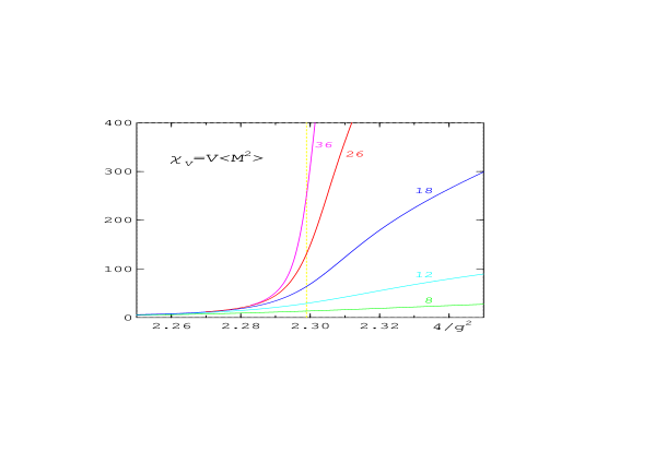
Figure 2: The finite volume susceptibility $\chi_{v}$ as function of $4/g^{2}$. The numbers indicate $N_{\sigma}$ and the vertical line shows the location of the critical point.

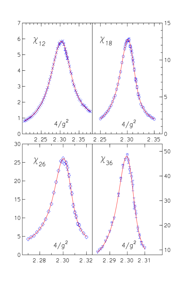
Figure 3: The susceptibility $\chi$ as function of $4/g^{2}$. The index on $\chi$ is $N_{\sigma}$, the lines are the DSM interpolations.

As was the case for the $3d$ Ising model [2], the simulations in the symmetric phase required fewer measurements for the same accuracy. This is observed also in Fig. 3, where the errors for $\bar{t}>0$ are larger than for $\bar{t}<0$, though we made in general more measurements there. In Fig. 4 we compare the results for $\chi$ for the different volumes.

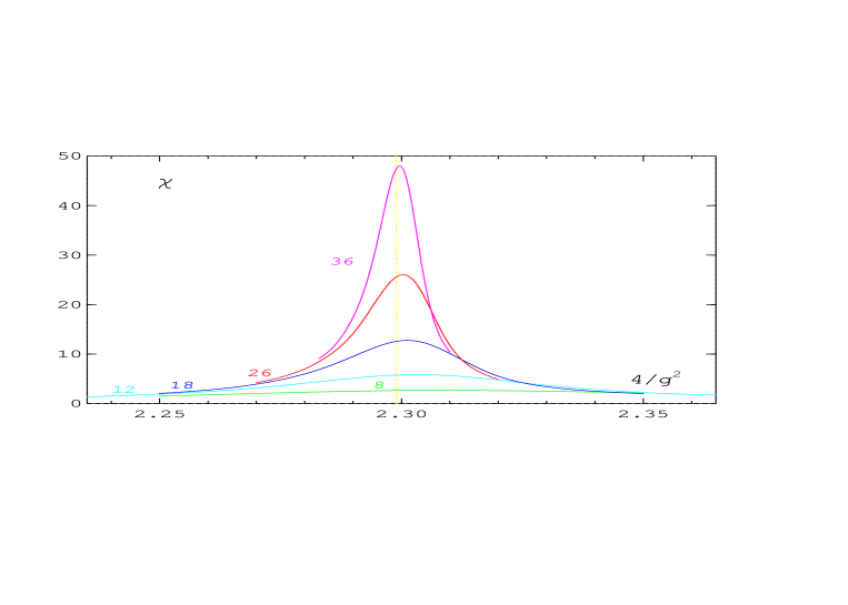
Figure 4: The susceptibility $\chi$ as function of $4/g^{2}$. The numbers are $N_{\sigma}$, the lines are the DSM interpolations and the dashed line shows the location of the critical point.

4 Scaling analysis of the data

4.1 The critical point

For our scaling analysis it is important to know the exact location of the critical point. We have therefore repeated the determination of the critical point with our new data and the $\chi^{2}-$method as proposed in ref. [12]. That method is a test on the $L-$dependence of an observable $O$ at the critical point $t=0,x=0$

$$O(t=0,L)=L^{\rho/\nu}\cdot\left(Q_{0}(0)+L^{-\omega}Q_{1}(0)\right)~{}.$$ (4.1)

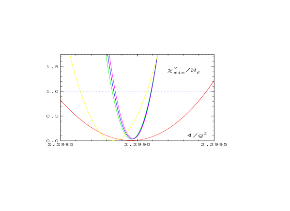
Figure 5: The minimal $\chi^{2}$ per degree of freedom for fits of ${\langle|M|\rangle}$ at fixed $4/g^{2}$ according to eq. 4.1: from [12](red); fit of new data, leading term only(yellow) and full fit with $\omega=1.1,1.2,1.3$ (green,blue,magenta).

If $x\not=0$ the $L-$dependence is drastically changed. At the critical point a fit to the form 4.1 has therefore the least minimal $\chi^{2}$ . Taking into account only the leading term in 4.1, a fit of ln$O$ as a function of ln$L$ gives at the same time the value of $\rho/\nu$. The results for $\beta/\nu$ and $\gamma/\nu$ in [12] were each about 1$\%$ off the values calculated from the Ising exponents used in ref. [2]

$$\beta=0.327~{},~{}~{}\gamma=1.239~{},~{}~{}\nu=0.631~{},$$ (4.2)

though the hyperscaling relation $d=2\beta/\nu+\gamma/\nu~{}$ was fulfilled up to 0.2$\%$. The set of data we have used in the current critical point analysis consisted of the new $L=12,18,26$ data and a new sample for $L=8$ calculated in the range $4/g^{2}=2.296-2.302$; the $L=36$ data were omitted here, because close to the critical point still more statistics would have been needed. As expected the better data produced a narrower $\chi^{2}-$parabola, the minimum was shifted to a slightly smaller $4/g^{2}-$value, yet the 1$\%-$difference of the exponent ratios remained. The apparent problem with the universality prediction disappeared however, when we included a correction-to-scaling term like in eq. 4.1 into our fit, as it was done already in the case of the observable $g_{r}$. In fig. 5 we compare the different minimal $\chi^{2}-$curves for the observable ${\langle|M|\rangle}$. In the $\omega$ dependent fits and in the subsequent scaling analysis we used as input the same set of critical exponents as [2]. The corresponding minimal $\chi^{2}-$parabolae are even narrower than in the leading term fits, the result for $4/g^{2}_{c}$ is essentially independent of $\omega$ for $\omega=1.1-1.3$  and is equal to the critical coupling found already in ref. [12]

$$4/g_{c}^{2}=2.29895(10)~{}.$$ (4.3)

Using the observables $\chi_{v}$ and $g_{r}$ leads to similar, consistent results, preferring $\omega\approx 1.2$. Here one should note that we describe the whole correction-to-scaling contributions with a single term. Consequently, the value of $\omega$ is somewhat higher as expected from the relation $\theta=\omega\nu=0.51(3)$ [2].

4.2 The scaling functions

In Figs. 6 and 7 we show the scaling functions $Q=L^{-\rho/\nu}O$ as a function of $x=\bar{t}L^{1/\nu}$ for $O={\langle|M|\rangle},\chi_{v}$ and $\chi$. The remnant dependence of the scaling functions on the characteristic length scale $L$ is due to corrections to scaling. A consistent succession of curves at fixed $x$ for different $L$ emerged only after using very high statistics and many couplings for the reweighting. To estimate $Q_{0}(x)$ we perform linear fits in $y=L^{-\omega}$ of $Q(x,y)$ at fixed $x$. We find a remarkable difference in the correction-to-scaling behaviours in the two phases $\bar{t}<0$ and $\bar{t}>0$. In the symmetric phase, here for $\chi_{v}$, the correction-to-scaling contribution is indeed linear in $y$. The best value of $\omega$ is again about 1.2. In the broken phase the correction is certainly not linear in $y$ for small $L$, both in $Q_{M}$ and $Q_{\chi}$. Therefore we have estimated $Q_{0}$ here from the two largest lattices with $\omega$ in the range 1.1-1.3. As can be seen from Fig. 7 the signs of the correction-to-scaling contributions are different for the susceptibility in the two phases. The universal ratio for the correction-to-scaling amplitudes is therefore negative. From a high temperature expansion Butera and Comi [10] predict that the correction amplitude of the $N-$vector spin model $a_{1\chi}(N)$ is negative for $N\mbox{}_{\textstyle\sim}^{\textstyle<}2$. Our finding of a negative correction-to-scaling contribution in the symmetric phase is in accord with this statement for $N=1$.

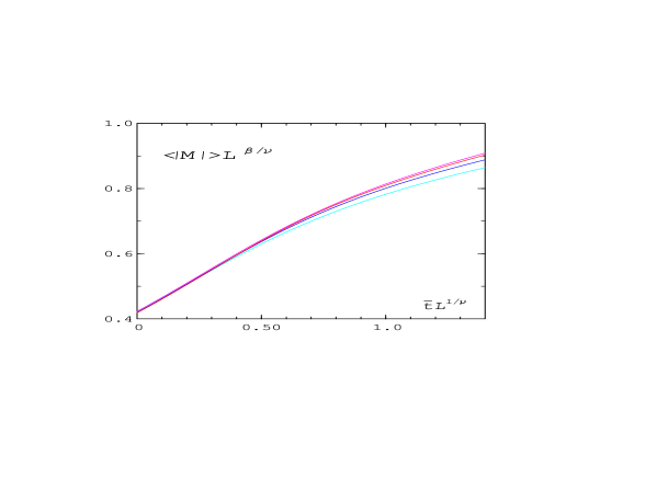
Figure 6: The scaling function ${\langle|M|\rangle}L^{\beta/\nu}$ vs. $x=\bar{t}L^{1/\nu}$ for $L=12$ (cyan), 18 (blue), 26 (red) and 36 (magenta).

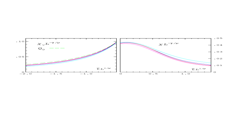
Figure 7: The scaling functions $\chi_{v}L^{-\gamma/\nu}$ (left) and $\chi L^{-\gamma/\nu}$ (right) vs. $x=\bar{t}L^{1/\nu}$ for $L=12$ (cyan), 18 (blue), 26 (red) and 36 (magenta). The green curve shows the estimated $Q_{0}(\chi_{v})$ for $\omega=1.2$ .

Kiskis [11] considered another interesting scaling function. It is defined by

$$h={{\langle M^{2}\rangle}\over{\langle|M|\rangle}^{2}}-1.$$ (4.4)

At the critical point $h$ is universal; there we find the value $h=0.240(5)$ from the $L=12,18,26$ lattices. In the strong coupling limit $4/g^{2}\rightarrow 0$ the function $h$ converges to $\pi/2-1$, because then the distribution of the magnetization is Gaussian [17]. This prediction can be checked in Fig. 8. At a fixed negative $x-$value the smallest lattice is at the lowest $4/g^{2}-$value. Correspondingly the result on the lattice with $L=12$ reaches the predicted value earlier.

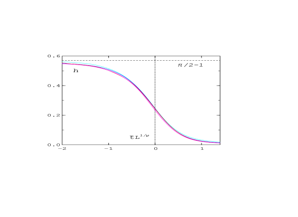
Figure 8: The scaling function $h$ vs. $x=\bar{t}L^{1/\nu}$ for $L=12$ (cyan), 18 (blue), 26 (red) and 36 (magenta).

4.3 The critical amplitudes

In Figs. 9-11 we show the functions $F_{O}$, eq. 2.30, which are obtained from the scaling functions $Q_{0}$ for ${\langle|M|\rangle},\chi_{v}$ and $\chi$, respectively. In determining $Q_{0}$ the Jackknife errors of the reweighted onservables were taken into account, the critical exponents from

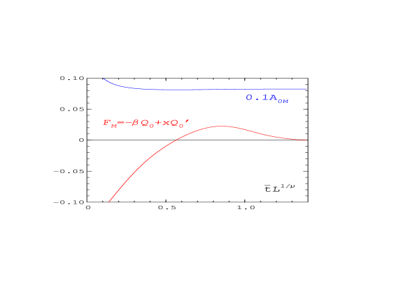
Figure 9: The control function $F_{M}$ (red) and the amplitude function $0.1A_{0M}$ (blue).

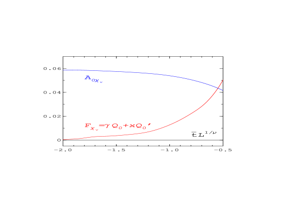
Figure 10: The control function $F_{\chi_{v}}$ (red) and the amplitude function $A_{0\chi_{v}}$ (blue).

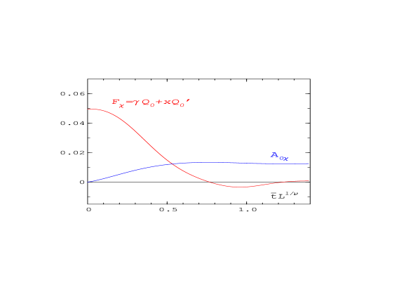
Figure 11: The control function $F_{\chi}$ (red) and the amplitude function $A_{0\chi}$ (blue).

the set 4.2 were used as input and $\omega$ was varied in the range 1.1-1.3 . The curves plotted in Figs. 9-11 correspond to $\omega=1.2$ .We observe again a different behaviour below and above the critical point. Whereas in the broken phase ($\bar{t}>0$) both the control functions $F_{M}$ and $F_{\chi}$ have a single zero at small $x$ and become essentially zero already around $x=1.4$, the approach to asymptopia in the symmetric phase (for $\chi_{v}$) is much slower. There the asymptotic region is reached only at $x\mbox{}_{\textstyle\sim}^{\textstyle<}-2$. The different behaviours are reflected as well in the amplitude functions $A_{0}$ which are also shown in the figures. We may now obtain the critical amplitudes from the amplitude functions in the asymptotic domain where $F_{O}$ is compatible with zero. We find

$$~{}~{}~{}B~{} = 0.825(1)~{},$$

$$~{}~{}~{}C_{+} = 0.0587(8)~{},$$

$$~{}~{}~{}C_{-} = 0.01243(12)~{}.$$

This amounts to a universal ratio for the susceptibility of

$$C_{+}/C_{-}=4.72(11)~{}.$$ (4.5)

The errors in the amplitudes come from different sources. Apart from the errors in $A_{0}$ due to errors from the data, the main error comes from variations in $\omega$ and errors from the point of onset of the asymptotic region. That leads to a bigger error for $C_{+}$ than for the other quantities. Our result for $C_{+}/C_{-}$ agrees nicely with the $3d$ Ising model value 4.75(3) of [2] and the latest field theoretic value 4.79(10) of [9].

From our envelope formula 2.23 we can even derive an estimate for the next-to-leading amplitude

$$a_{1}=|x|^{-\omega\nu}Q_{1}(x)/Q_{0}(x)~{}.$$ (4.6)

Though variations of $\omega$ influence strongly these correction-to-scaling amplitudes, their ratio is less affected. For the susceptibility we obtain the amplitude ratio $~{}a_{1+}/a_{1-}=-0.37(2)~{}$. As discussed already this ratio is negative. The overall size of the ratio is however of comparable magnitude to other estimates [18].

5 Summary and conclusion

We have shown that it is possible to determine critical point amplitudes in $SU(2)$ from Monte Carlo simulations in finite, not extremely large volumes.

Very accurate data are however required for the necessary estimate of correction-to-scaling contributions to the scaling functions and the control of their approach to asymptopia.

In the symmetric phase and in the broken phase we find different correction-to-scaling dependencies of the scaling functions.

Our result for $C_{+}/C_{-}$ is in excellent agreement with the $3d$ Ising model value from Monte Carlo simulations and field theory calculations of the $N=1-$vector model. The agreement of this critical amplitude ratio for the (3+1) dimensional $SU(2)$ gauge theory and the $3d$ Ising model is a further strong support of the universality hypothesis of Svetitsky and Yaffe [19] beyond the level of critical exponents.

Acknowledgements

We thank David Miller for a careful reading of the manuscript.

Appendix

In Tables 2-7 we present more details on our Monte Carlo simulations.

$4/g^{2}$	$N_{m}$	$\langle|M|\rangle$	$\chi_{v}$	$\Delta\chi_{v}$	$\chi$	$\Delta\chi$	$g_{r}$
2.28300	20000	0.0189 (02)	25.7	0.6	9.05	0.21	-0.167 (45)
2.28400	30501	0.0198 (02)	28.2	0.4	9.87	0.21	-0.240 (50)
2.28500	20000	0.0200 (02)	29.0	0.6	10.43	0.26	-0.153 (34)
2.28600	30000	0.0210 (02)	31.8	0.5	11.23	0.22	-0.176 (52)
2.28750	30000	0.0237 (02)	39.6	0.6	13.51	0.24	-0.316 (48)
2.28850	30000	0.0248 (02)	43.7	0.9	15.07	0.35	-0.287 (22)
2.29000	29436	0.0270 (05)	51.4	1.6	17.48	0.54	-0.346 (44)
2.29120	32180	0.0294 (06)	60.9	2.3	20.67	0.73	-0.368 (42)
2.29250	36751	0.0319 (04)	70.3	1.4	22.85	0.42	-0.540 (51)
2.29500	26350	0.0409 (05)	110.6	2.3	32.40	0.71	-0.818 (34)
2.29630	30000	0.0473 (08)	143.1	3.8	38.72	0.82	-0.974 (36)
2.29750	40107	0.0553 (09)	186.7	4.6	44.02	0.79	-1.191 (27)
2.29880	61070	0.0656 (11)	247.5	6.7	46.64	0.54	-1.400 (21)
2.30000	57600	0.0738 (11)	302.1	6.8	48.27	0.87	-1.522 (20)
2.30060	35000	0.0809 (11)	351.5	7.5	45.99	0.96	-1.618 (15)
2.30130	36051	0.0881 (11)	404.4	7.8	42.41	1.44	-1.699 (15)
2.30250	35622	0.0963 (10)	472.4	7.7	39.53	1.94	-1.759 (13)
2.30320	41213	0.1023 (10)	524.8	7.6	36.12	2.15	-1.806 (11)
2.30380	32000	0.1085 (10)	577.9	8.2	28.91	2.22	-1.852 (11)
2.30440	41400	0.1113 (05)	605.7	4.8	27.28	0.94	-1.861 (04)
2.30500	33600	0.1163 (05)	655.7	5.1	24.46	1.39	-1.885 (05)
2.30600	20430	0.1224 (07)	717.6	6.6	18.54	1.10	-1.914 (04)
2.30700	20000	0.1279 (06)	778.8	6.0	15.57	0.95	-1.930 (04)
2.30800	20000	0.1334 (05)	843.0	6.1	12.79	0.73	-1.945 (03)
2.30900	25513	0.1377 (02)	896.5	2.6	11.55	0.31	-1.953 (01)
2.31000	20272	0.1422 (05)	954.3	5.7	10.74	0.52	-1.959 (02)

Table 2: The data from the $36^{3}\times 4$ lattice.

$4/g^{2}$	$N_{m}$	$\langle|M|\rangle$	$\chi_{v}$	$\Delta\chi_{v}$	$\chi$	$\Delta\chi$	$g_{r}$
2.27000	30000	0.0207 (2)	11.8	0.2	4.25	0.06	-0.082 (38)
2.27250	30518	0.0221 (2)	13.4	0.2	4.77	0.07	-0.121 (37)
2.27500	30043	0.0233 (2)	14.7	0.2	5.18	0.08	-0.161 (44)
2.27750	20800	0.0254 (3)	17.5	0.4	6.14	0.15	-0.215 (27)
2.28000	30000	0.0273 (2)	20.1	0.4	7.09	0.15	-0.245 (14)
2.28250	20800	0.0298 (5)	23.9	0.7	8.23	0.24	-0.270 (46)
2.28500	24204	0.0329 (4)	28.7	0.7	9.65	0.25	-0.432 (38)
2.28750	20000	0.0369 (7)	35.6	1.3	11.74	0.35	-0.472 (41)
2.29000	25000	0.0420 (5)	44.8	0.7	13.77	0.21	-0.686 (37)
2.29200	30000	0.0470 (7)	55.6	1.4	16.83	0.27	-0.744 (35)
2.29400	41525	0.0543 (8)	71.6	1.8	19.68	0.17	-0.955 (28)
2.29600	60000	0.0626 (4)	91.6	1.0	22.76	0.29	-1.134 (11)
2.29800	70000	0.0718 (4)	115.9	0.9	25.36	0.14	-1.281 (08)
2.29900	40004	0.0782 (6)	132.6	1.6	25.19	0.27	-1.405 (12)
2.30000	70000	0.0832 (4)	147.7	1.0	26.11	0.31	-1.456 (09)
2.30120	59446	0.0922 (4)	174.0	1.6	24.64	0.28	-1.582 (04)
2.30250	60761	0.0984 (7)	195.0	2.4	24.97	0.40	-1.630 (09)
2.30370	60000	0.1069 (9)	224.3	2.6	23.57	0.71	-1.703 (11)
2.30500	81780	0.1146 (6)	252.5	1.8	21.50	0.53	-1.760 (06)
2.30620	60000	0.1218 (8)	279.2	2.8	18.58	0.71	-1.808 (08)
2.30750	81059	0.1288 (5)	308.2	1.7	16.61	0.47	-1.845 (04)
2.30870	40000	0.1352 (4)	334.7	1.4	13.39	0.54	-1.876 (04)
2.31000	38400	0.1414 (5)	362.9	2.2	11.49	0.39	-1.899 (03)
2.31120	60000	0.1461 (3)	385.7	1.1	10.36	0.47	-1.913 (03)
2.31250	35000	0.1511 (3)	409.7	1.5	8.39	0.41	-1.929 (02)
2.31380	20000	0.1553 (5)	431.9	2.6	8.05	0.39	-1.936 (02)
2.31500	20000	0.1595 (6)	454.2	2.8	6.81	0.35	-1.946 (03)
2.31750	20000	0.1672 (4)	497.3	2.0	5.84	0.24	-1.957 (02)
2.32000	20000	0.1743 (2)	538.8	1.2	4.81	0.07	-1.966 (00)

Table 3: The data from the $26^{3}\times 4$ lattice.

$4/g^{2}$	$N_{m}$	$\langle|M|\rangle$	$\chi_{v}$	$\chi$	$g_{r}$
2.25000	20000	0.0253 (01)	5.79   (08)	2.05 (04)	-0.137 (23)
2.25250	20000	0.0265 (01)	6.33   (06)	2.24 (03)	-0.208 (23)
2.25500	25000	0.0271 (02)	6.64   (08)	2.36 (03)	-0.146 (42)
2.25750	21500	0.0280 (02)	7.10   (09)	2.53 (04)	-0.127 (21)
2.26000	32816	0.0293 (02)	7.78   (12)	2.77 (05)	-0.127 (18)
2.26250	22497	0.0308 (02)	8.52   (12)	2.99 (05)	-0.200 (29)
2.26500	30000	0.0321 (02)	9.21   (13)	3.21 (04)	-0.212 (21)
2.26750	30857	0.0342 (02)	10.40   (11)	3.58 (04)	-0.302 (20)
2.27000	20000	0.0355 (03)	11.22   (19)	3.86 (07)	-0.286 (38)
2.27250	20200	0.0382 (04)	12.84   (23)	4.35 (06)	-0.353 (28)
2.27500	20000	0.0404 (04)	14.38   (23)	4.87 (08)	-0.382 (29)
2.27750	20000	0.0426 (05)	15.78   (30)	5.20 (07)	-0.489 (31)
2.28000	20000	0.0464 (03)	18.60   (25)	6.03 (11)	-0.539 (26)
2.28250	20000	0.0494 (03)	20.95   (25)	6.72 (08)	-0.598 (22)
2.28500	20000	0.0536 (05)	24.35   (41)	7.59 (11)	-0.673 (24)
2.28750	20490	0.0581 (05)	28.06   (43)	8.40 (08)	-0.771 (27)
2.29000	30000	0.0654 (10)	34.61   (81)	9.64 (09)	-0.934 (37)
2.29250	25000	0.0718 (06)	40.58   (62)	10.49 (13)	-1.067 (16)
2.29500	30075	0.0796 (05)	48.40   (46)	11.49 (11)	-1.182 (15)
2.29600	30000	0.0839 (06)	52.92   (67)	11.85 (11)	-1.261 (11)
2.29700	30000	0.0851 (09)	54.38   (93)	12.18 (17)	-1.260 (15)
2.29800	45000	0.0890 (09)	58.48   (79)	12.32 (13)	-1.315 (20)
2.29900	45000	0.0946 (06)	64.72   (68)	12.59 (09)	-1.387 (08)
2.30000	45000	0.0990 (06)	69.71   (61)	12.61 (14)	-1.441 (11)
2.30200	50151	0.1064 (10)	78.73 (115)	12.68 (24)	-1.518 (14)

Table 4: List(a) of data from the $18^{3}\times 4$ lattice.

$4/g^{2}$	$N_{m}$	$\langle|M|\rangle$	$\chi_{v}$	$\chi$	$g_{r}$
2.30350	50856	0.1113 (08)	84.92   (85)	12.74 (27)	-1.560 (14)
2.30500	49940	0.1208 (09)	96.95 (106)	11.85 (19)	-1.643 (09)
2.30600	39257	0.1232 (06)	100.36   (73)	11.87 (17)	-1.660 (07)
2.30700	20157	0.1269 (08)	105.25 (107)	11.40 (30)	-1.686 (09)
2.30850	40574	0.1336 (08)	115.04 (101)	10.97 (34)	-1.728 (08)
2.31000	40000	0.1395 (09)	123.64 (117)	10.15 (28)	-1.765 (07)
2.31100	20000	0.1434 (12)	129.55 (165)	9.70 (35)	-1.785 (08)
2.31300	40000	0.1506 (05)	140.89   (72)	8.70 (23)	-1.820 (03)
2.31500	30000	0.1586 (04)	154.14   (52)	7.39 (24)	-1.854 (03)
2.31650	25000	0.1617 (06)	159.70   (87)	7.21 (29)	-1.863 (04)
2.31800	20115	0.1668 (05)	168.54   (81)	6.32 (22)	-1.882 (02)
2.32000	30000	0.1728 (05)	179.55   (91)	5.37 (19)	-1.902 (03)
2.32200	22721	0.1780 (05)	189.71   (79)	4.98 (29)	-1.914 (03)
2.32500	20000	0.1851 (03)	203.80   (53)	4.03 (11)	-1.931 (01)
2.32750	20000	0.1900 (02)	214.13   (38)	3.67 (09)	-1.939 (01)
2.33000	21071	0.1949 (02)	225.07   (38)	3.53 (13)	-1.945 (01)
2.33250	20000	0.1992 (02)	234.60   (48)	3.09 (08)	-1.952 (01)
2.33500	20015	0.2042 (02)	245.93   (35)	2.85 (03)	-1.957 (00)
2.33750	20000	0.2080 (02)	254.92   (49)	2.57 (05)	-1.962 (01)
2.34000	20000	0.2118 (01)	264.19   (31)	2.51 (05)	-1.965 (00)
2.34250	20000	0.2154 (03)	273.05   (62)	2.40 (04)	-1.967 (01)
2.34500	20026	0.2191 (02)	282.24   (48)	2.18 (02)	-1.970 (00)
2.34750	20000	0.2224 (02)	290.62   (43)	2.15 (01)	-1.972 (00)
2.35000	20086	0.2257 (02)	299.15   (40)	2.00 (04)	-1.974 (00)

Table 5: List(b) of data from the $18^{3}\times 4$ lattice.

$4/g^{2}$	$N_{m}$	$\langle|M|\rangle$	$\chi_{v}$	$\chi$	$g_{r}$
2.20500	20000	0.0286 (1)	2.22 (01)	0.80 (1)	-0.058 (50)
2.20750	20000	0.0294 (2)	2.34 (03)	0.85 (1)	-0.012 (34)
2.21000	20460	0.0300 (1)	2.41 (02)	0.85 (1)	-0.123 (43)
2.21250	20000	0.0304 (2)	2.51 (03)	0.91 (1)	-0.026 (39)
2.21500	20000	0.0311 (2)	2.61 (03)	0.94 (1)	-0.109 (39)
2.21750	20000	0.0319 (1)	2.75 (02)	0.99 (1)	-0.081 (25)
2.22000	20000	0.0326 (2)	2.87 (04)	1.03 (1)	-0.069 (57)
2.22250	20512	0.0335 (2)	3.00 (03)	1.06 (1)	-0.166 (29)
2.22500	20000	0.0339 (2)	3.09 (03)	1.11 (1)	-0.085 (31)
2.22750	20000	0.0350 (1)	3.28 (02)	1.17 (1)	-0.114 (22)
2.23000	20000	0.0362 (1)	3.51 (02)	1.25 (1)	-0.156 (32)
2.23250	20498	0.0370 (2)	3.66 (04)	1.29 (1)	-0.172 (14)
2.23500	20014	0.0382 (3)	3.88 (05)	1.36 (2)	-0.224 (28)
2.23750	20000	0.0392 (3)	4.08 (05)	1.43 (1)	-0.207 (36)
2.24000	20000	0.0406 (2)	4.36 (04)	1.52 (1)	-0.250 (35)
2.24250	20000	0.0422 (2)	4.71 (05)	1.64 (2)	-0.261 (19)
2.24500	20000	0.0431 (2)	4.92 (05)	1.71 (3)	-0.284 (31)
2.24750	20000	0.0443 (3)	5.20 (06)	1.81 (2)	-0.261 (23)
2.25000	20000	0.0459 (3)	5.54 (06)	1.90 (2)	-0.328 (06)
2.25250	20000	0.0470 (4)	5.81 (08)	1.99 (3)	-0.347 (32)
2.25500	20000	0.0488 (2)	6.27 (06)	2.16 (3)	-0.329 (14)
2.25750	20000	0.0513 (3)	6.83 (05)	2.28 (1)	-0.449 (23)
2.26000	20974	0.0533 (4)	7.34 (07)	2.43 (2)	-0.453 (26)
2.26250	20000	0.0556 (4)	7.95 (11)	2.61 (3)	-0.498 (14)
2.26500	20000	0.0576 (5)	8.52 (12)	2.79 (3)	-0.529 (17)
2.26750	26000	0.0607 (4)	9.29 (10)	2.92 (3)	-0.603 (11)
2.27000	20000	0.0640 (4)	10.29 (12)	3.21 (3)	-0.660 (18)
2.27250	20000	0.0669 (6)	11.16 (16)	3.43 (3)	-0.697 (21)
2.27500	20000	0.0690 (3)	11.83 (11)	3.61 (4)	-0.724 (17)
2.27750	20000	0.0730 (7)	13.07 (21)	3.87 (4)	-0.803 (21)
2.28000	20056	0.0764 (3)	14.22 (11)	4.14 (4)	-0.839 (09)
2.28250	20000	0.0814 (8)	15.85 (27)	4.40 (4)	-0.931 (16)
2.28500	20415	0.0858 (6)	17.40 (20)	4.67 (4)	-1.009 (18)
2.28750	20000	0.0904 (7)	18.97 (21)	4.86 (4)	-1.079 (17)
2.29000	40000	0.0952 (3)	20.78 (09)	5.13 (4)	-1.129 (09)
2.29250	40000	0.1014 (8)	23.17 (29)	5.39 (4)	-1.207 (13)
2.29500	40000	0.1066 (9)	25.12 (30)	5.50 (4)	-1.277 (15)

Table 6: List(a) of data from the $12^{3}\times 4$ lattice.

$4/g^{2}$	$N_{m}$	$\langle|M|\rangle$	$\chi_{v}$	$\chi$	$g_{r}$
2.29700	40000	0.1105 (6)	26.80 (22)	5.70 (04)	-1.308 (09)
2.29800	40000	0.1129 (8)	27.66 (27)	5.62 (04)	-1.344 (11)
2.29900	50000	0.1165 (5)	29.19 (17)	5.74 (03)	-1.375 (07)
2.30000	30000	0.1193 (6)	30.29 (20)	5.71 (05)	-1.407 (08)
2.30200	30107	0.1234 (8)	32.16 (35)	5.84 (05)	-1.439 (10)
2.30500	30000	0.1326 (7)	36.17 (29)	5.78 (05)	-1.522 (08)
2.30700	50000	0.1362 (7)	37.90 (31)	5.86 (05)	-1.540 (07)
2.31000	30000	0.1447 (9)	41.85 (37)	5.66 (09)	-1.604 (09)
2.31300	20000	0.1546 (8)	46.66 (37)	5.35 (09)	-1.668 (07)
2.31500	20000	0.1592 (8)	48.96 (35)	5.15 (12)	-1.694 (07)
2.31700	20000	0.1636 (12)	51.26 (56)	5.01 (15)	-1.717 (09)
2.31900	20000	0.1687 (5)	53.96 (24)	4.79 (10)	-1.742 (04)
2.32000	20000	0.1707 (8)	55.11 (40)	4.75 (08)	-1.750 (04)
2.32250	20000	0.1754 (8)	57.66 (40)	4.53 (06)	-1.772 (04)
2.32500	39432	0.1814 (5)	61.15 (26)	4.27 (06)	-1.795 (03)
2.32750	40000	0.1879 (5)	64.94 (25)	3.92 (08)	-1.821 (03)
2.33000	40000	0.1917 (3)	67.30 (18)	3.80 (04)	-1.832 (01)
2.33250	20000	0.1976 (4)	70.84 (24)	3.34 (04)	-1.854 (02)
2.33500	40000	0.2019 (5)	73.54 (30)	3.13 (06)	-1.866 (03)
2.33750	39618	0.2063 (4)	76.59 (25)	3.02 (06)	-1.876 (02)
2.34000	20000	0.2106 (5)	79.38 (35)	2.74 (06)	-1.888 (02)
2.34250	20000	0.2139 (3)	81.72 (20)	2.63 (07)	-1.896 (02)
2.34500	18371	0.2180 (2)	84.60 (14)	2.48 (07)	-1.904 (01)
2.34750	20000	0.2210 (3)	86.76 (20)	2.35 (06)	-1.908 (02)
2.35000	20000	0.2249 (2)	89.62 (17)	2.19 (05)	-1.916 (01)
2.35250	20000	0.2283 (4)	92.19 (30)	2.13 (06)	-1.921 (02)
2.35500	20000	0.2305 (3)	93.86 (20)	2.07 (06)	-1.924 (01)
2.35750	20000	0.2342 (3)	96.65 (20)	1.87 (03)	-1.931 (01)
2.36000	20000	0.2365 (4)	98.47 (24)	1.85 (06)	-1.933 (02)
2.36250	20000	0.2395 (3)	100.89 (24)	1.79 (07)	-1.937 (02)
2.36500	20000	0.2414 (3)	102.50 (25)	1.77 (06)	-1.939 (01)
2.36750	20222	0.2441 (2)	104.61 (19)	1.67 (04)	-1.942 (01)
2.37000	20000	0.2467 (3)	106.80 (24)	1.63 (04)	-1.945 (01)
2.37250	20000	0.2493 (3)	108.95 (21)	1.53 (03)	-1.948 (01)
2.37500	20000	0.2515 (3)	110.75 (23)	1.47 (02)	-1.950 (01)
2.37750	20000	0.2543 (2)	113.19 (21)	1.44 (02)	-1.953 (00)
2.38000	20000	0.2563 (3)	114.96 (24)	1.41 (02)	-1.954 (01)

Table 7: List(b) of data from the $12^{3}\times 4$ lattice.

References

- [1] V. Privman, P.C. Hohenberg, A. Aharony, Universal Critical Point Amplitude Relations, in ”Phase Transitions and Critical Phenomena”, vol. 14, C. Domb and J.L. Lebowitz eds. (Academic Press 1991).
- [2] M. Caselle and M. Hasenbusch, J. Phys. A30 (1997) 4963; Nucl. Phys. B(Proc.Suppl.)63 (1998) 613.
- [3] E. Brezin, J.-C. LeGuillou and J. Zinn-Justin, Phys. Lett. 47A (1974) 285.
- [4] A. Aharony and P.C. Hohenberg, Phys. Rev. B13 (1976) 3081.
- [5] P.C. Albright and J.F. Nicoll, Phys. Rev. B31 (1985) 4576.
- [6] C. Bervillier, Phys. Rev. B34 (1986) 8141.
- [7] C. Bagnuls, C. Bervillier, D.I. Meiron and B.G. Nickel, Phys. Rev. B35 (1987)3585.
- [8] R. Guida and J. Zinn-Justin, Nucl. Phys. B489[FS] (1997) 626.
- [9] R. Guida and J. Zinn-Justin,Critical exponents of the N-vector model, Preprint SPhT-t97/040, cond-mat/9803240 v2.
- [10] P. Butera and M. Comi, hep-lat/9805025.
- [11] J. Kiskis, Phys. Rev. D45 (1992) 4640.
- [12] J. Engels, S. Mashkevich, T. Scheideler and G. Zinovjev, Phys. Lett. B365 (1996) 219.
- [13] M.N. Barber, in ”Phase Transitions and Critical Phenomena”, vol. 8, C. Domb and J.L. Lebowitz eds. (Academic Press 1983).
- [14] A.L. Talapov and H.W.J. Blöte, J. Phys. A29 (1996) 5727.
- [15] J. Engels, J. Fingberg and D.E. Miller, Nucl. Phys. B387 (1992) 501.
-
[16]
M. Falconi, E. Marinari, M.L. Paciello,
G. Parisi and B. Taglienti, Phys. Lett. 108B (1982) 331;
E. Marinari, Nucl. Phys. B235 (1984) 123;
G. Bhanot, S. Black, P. Carter and R. Salvador, Phys. Lett. 183B (1986) 331;
A.M. Ferrenberg and R.H. Swendsen, Phys. Rev. Lett. 61 (1988) 2635; 63 (1989) 1195. - [17] J. Kiskis, private communication.
- [18] J. Zinn-Justin, Quantum field theory and critical phenomena (1993) Clarendon Press, Oxford.
- [19] B. Svetitsky and G. Yaffe, Nucl. Phys. B210FS6 (1982) 423.