Probing finite size effects in $\left(\lambda\Phi^{4}\right)_{4}$ MonteCarlo calculations

Abstract

The Constrained Effective Potential (CEP) is known to be equivalent to the usual Effective Potential (EP) in the infinite volume limit. We have carried out MonteCarlo calculations based on the two different definitions to get informations on finite size effects. We also compared these calculations with those based on an Improved CEP (ICEP) which takes into account the finite size of the lattice. It turns out that ICEP actually reduces the finite size effects which are more visible near the vanishing of the external source.

1 CEP and its properties

The effective potential is defined as the Legendre transform of the Schwinger function $W\left(\Omega,j\right)$ ($j$ constant external source, $\Omega$ lattice size)

$$\Gamma\left(\Omega,\bar{\phi}\right)=\sup_{j}\left(j\bar{\phi}-W\left(\Omega,j\right)\right)$$ (1)

with

$$\exp\left(\Omega W\left(\Omega,j\right)\right)=$$

$$\int\mathcal{D}\phi\exp\left\{-S\left[\phi\right]+\Omega j\mathcal{M}\left[\phi\right]\right\}$$

$$\mathcal{M}\left[\phi\right] = \frac{1}{\Omega}\int_{\Omega}\phi\left(x\right)\mathrm{d}^{d}x$$

$$S\left[\phi\right] = \int_{\Omega}\left(\frac{1}{2}\left(\partial_{\mu}\phi\right)^{2}+V\left[\phi\right]\right)\mathrm{d}^{d}x$$

$$V\left[\phi\right] = \frac{1}{2}\mathrm{r}_{0}\phi^{2}+\frac{1}{4}\lambda_{0}\phi^{4}.$$

According to ref. [1] the CEP $U\left(\Omega,\bar{\phi}\right)$ is defined as

$$\exp\left(-\Omega U\left(\Omega,\bar{\phi}\right)\right)=$$ (2)

$$\int\mathcal{D}\phi\delta\left(\mathcal{M}\left[\phi\right]-\bar{\phi}\right)\times\exp\left(-S\left[\phi\right]\right)\equiv\mathcal{N}$$

which entails

$$\exp\left(\Omega W\left(\Omega,j\right)\right)=$$ (3)

$$\int\mathrm{d}\bar{\phi}\exp\left[\Omega\left(j\bar{\phi}-U\left(\Omega,\bar{\phi}\right)\right)\right]$$

it has been shown in [1] that

$$\lim_{\Omega\to\infty}\Gamma\left(\Omega,\bar{\phi}\right)=\lim_{\Omega\to\infty}U\left(\Omega,\bar{\phi}\right).$$ (4)

2 Using CEP on the lattice

If $\Omega$ is large enough, from eq. (4) we get

$$\Gamma\left(\Omega,\bar{\phi}\right)\approx U\left(\Omega,\bar{\phi}\right)$$

and

$$J=\frac{\mathrm{d}\Gamma\left(\Omega,\bar{\phi}\right)}{\mathrm{d}\bar{\phi}}\approx\frac{\mathrm{d}U\left(\Omega,\bar{\phi}\right)}{\mathrm{d}\bar{\phi}}.$$

We define

$$\left\langle O\left[\phi\right]\right\rangle_{\bar{\phi}}=$$

$$\frac{1}{\mathcal{N}}\int\mathcal{D}\phi\delta\left(\mathcal{M}\left[\phi\right]-\bar{\phi}\right)O\left[\phi\right]\exp\left(-S\left[\phi\right]\right)$$

From [1] CEP gives

$$\frac{\mathrm{d}U\left(\Omega,\bar{\phi}\right)}{\mathrm{d}\bar{\phi}}=\frac{1}{\Omega}\left\langle\int\mathrm{d}^{d}xV^{\prime}\left[\phi\right]\right\rangle_{\bar{\phi}}=\left\langle\mathcal{V}^{\prime}\right\rangle_{\bar{\phi}}\approx J$$

3 Improving CEP

We evaluate eq. (3) with the saddle point method around a $\varphi$ such that $j-U^{\prime}\left(\Omega,\varphi\right)=0$. Then we get

$$W\left(\Omega,j\right) = j\varphi-U\left(\Omega,\varphi\right)-$$

$$\frac{1}{2}\frac{1}{\Omega}\ln U^{\prime\prime}\left(\Omega,\varphi\right)+$$

$$\frac{1}{2}\frac{1}{\Omega}\ln 2\pi-\frac{1}{2}\frac{1}{\Omega}\ln\Omega.$$

From above equation and from eq. (1) then one has

$$\Gamma\left(\Omega,\varphi\right) = U\left(\Omega,\varphi\right)+\frac{1}{2}\frac{1}{\Omega}\ln U^{\prime\prime}\left(\Omega,\varphi\right)-$$

$$\frac{1}{2}\frac{1}{\Omega}\ln 2\pi+\frac{1}{2}\frac{1}{\Omega}\ln\Omega$$

and hence

$$j=\frac{\mathrm{d}\Gamma\left(\Omega,\varphi\right)}{\mathrm{d}\varphi}=U^{\prime}\left(\Omega,\varphi\right)+\frac{1}{2}\frac{1}{\Omega}\frac{U^{\prime\prime\prime}\left(\Omega,\varphi\right)}{U^{\prime\prime}\left(\Omega,\varphi\right)}$$ (6)

Iteration of the method adopted for computing $U^{\prime}\left(\Omega,\varphi\right)$ gives

$$U^{\prime\prime} = \left\langle\mathcal{V}^{\prime\prime}\right\rangle_{\bar{\phi}}-\Omega\left\langle\left(\mathcal{V}^{\prime}-\left\langle\mathcal{V}^{\prime}\right\rangle_{\bar{\phi}}\right)^{2}\right\rangle_{\bar{\phi}}$$

$$U^{\prime\prime\prime} = \left\langle\mathcal{V}^{\prime\prime\prime}\right\rangle_{\bar{\phi}}-$$

$$3\Omega\left\langle\left(\mathcal{V}^{\prime}-\left\langle\mathcal{V}^{\prime}\right\rangle_{\bar{\phi}}\right)\left(\mathcal{V}^{\prime\prime}-\left\langle\mathcal{V}^{\prime\prime}\right\rangle_{\bar{\phi}}\right)\right\rangle_{\bar{\phi}}+$$

$$\Omega^{2}\left\langle\left(\mathcal{V}^{\prime}-\left\langle\mathcal{V}^{\prime}\right\rangle_{\bar{\phi}}\right)^{3}\right\rangle_{\bar{\phi}}$$

4 Montecarlo for CEP and ICEP and data analysis

The Montecarlo updating must be performed by keeping constant the $\bar{\phi}$ value.

This can be achieved by doing the Montecarlo update on pairs of lattice sites in such a way that changing the field values does not change their average.

In [1] this was done by choosing a fixed site and pairing it with the others in turn.

We developed a different algorithm, which performs, for each site of the lattice, a random choice of the second site. This avoids some problems concerning next neighbor updates and, moreover, allows encoding either in vectorial or parallel programs.

Our procedure to get an estimate of finite size effects in Montecarlo computations is summarized as follows

$$\begin{array}[]{cccl}J^{\mathrm{IN}}&\stackrel{{\scriptstyle\mathrm{EP}}}{{\longrightarrow}}&\left\langle\phi\right\rangle^{\mathrm{OUT}}&\\ &&\leavevmode\hbox{\begin{minipage}[t]{28.45274pt} $\displaystyle\downarrow$ \end{minipage}}&\begin{array}[]{l}\mathrm{mean}\\ \mathrm{value}\end{array}\\ J^{\mathrm{OUT}}&\stackrel{{\scriptstyle\leavevmode\hbox{\begin{minipage}[t]{28.45274pt} \begin{center} CEP \\ ICEP \end{center} \end{minipage}}}}{{\longleftarrow}}&\left\langle\phi\right\rangle^{\mathrm{IN}}&\end{array}$$

$J^{\mathrm{IN}}$ is the input value of standard Montecarlo Effective Potential (EP). In the infinite volume limit $J^{\mathrm{IN}}$ and $J^{\mathrm{OUT}}$, the latter given from CEP or ICEP, should be equal. Their difference, from finite lattice calculations, includes some finite size effects, which should be controlled with ICEP. The effectiveness of ICEP has been verified from the behavior of two parameters $\rho$ and $\epsilon$

$$\rho = \frac{\left\langle\phi\right\rangle^{\mathrm{IN}}J^{\mathrm{OUT}}}{\left\langle\phi\right\rangle^{\mathrm{OUT}}J^{\mathrm{IN}}}-1$$

$$\epsilon = 2\frac{J^{\mathrm{IN}}-J^{\mathrm{OUT}}}{J^{\mathrm{IN}}+J^{\mathrm{OUT}}}.$$

The errors in $\rho$ includes those of $\left\langle\phi\right\rangle^{\mathrm{OUT}}$ and $J^{\mathrm{OUT}}$. The errors in $\epsilon$ come from those in $J^{\mathrm{OUT}}$ only. The EP values used as input in our Montecarlo calculations are those reported in [2] supplemented with some others obtained by running the same program. They are also used to compare EP, CEP and ICEP in Fig. 1.

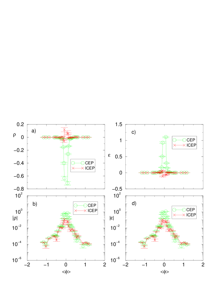
Figure 1: The lattice calculations have been performed with $\mathrm{r}_{0}$=-0.2279 and $\lambda_{0}$=0.5

5 Comments and conclusions

From the plots in Fig. 1 a similar behaviour of $\rho$ and $\epsilon$ is apparent, though only $\rho$ depends on EP calculations. The comparison of the usual Montecarlo EP with CEP and ICEP shows that the latter reduces the finite size effects, which should also affect EP. These effects are especially relevant when $\left\langle\phi\right\rangle\approx 0$ and in this domain the plots in Fig. 1 clearly show that ICEP is better than CEP.

References

• [1] R. Fukuda and E. Kyryakopoulos, Nucl. Phys. B85 354 (1975); L. O’Raifeartaigh, A. Wipf and H. Yoneyama, Nucl. Phys. B271 653 (1986)
• [2] A. Agodi, G. Andronico, P. Cea, M. Consoli and L. Cosmai, Mod. Phys. Lett. A12, 1011 (1997)