Determination of constant lattice spacing trajectories in lattice QCD

Abstract

We argue that lattice simulations of full QCD with varying quark mass are best conducted at fixed lattice spacing rather than at fixed $\beta$. We present techniques which enable this to be carried out effectively, namely the tuning in bare parameter space and efficient stochastic estimation of the fermion determinant. Results and tests of the method are presented. We discuss other applications of such techniques.

1 CONSTANT LATTICE SPACING

Hadron spectrum measurements by the UKQCD collaboration [1, 2] using an improved action have shown a surprisingly strong dependence of the effective lattice spacing on the bare quark mass. Recent preliminary measurements of the Sommer scale $r_{0}$ using the non-perturbatively improved value of $c_{\rm sw}$ in $16^{3}\times 32$ simulations [3] have confirmed this. See Table 1.

Table 1: Lattice spacing determined from $r_{0}$ [4] at $\beta=5.2$ for ${\cal O}(a)$-improved Wilson fermions

$\kappa$	$.1330$	$.1340$	$.1345$	$.1350$
$a$ [fm]	$.154(2)$	$.140(4)$	$.130(2)$	$.1173(16)$

Since the parameters in chiral perturbation theory inherit this underlying $a$-dependence, this complicates chiral extrapolations of simulation measurements and obscures comparisons with quenched calculations. Indeed, one would not attempt to compare quenched and full QCD at the same value of $\beta$. Because of the strong and non-trivial dependence on the the bare quark mass, one should avoid using fixed $\beta$ within the dynamical sector also.

With this in mind, we investigate how one might control the effective lattice spacing by tuning the bare action parameters while the effects of decreasing quark mass are studied. In previous work [5, 6] we have described how stochastic estimates of the fermion determinant may be used to tune action parameters so as to maintain fixed the value of some observable $F$. We would suggest that, in order to hold the effective lattice spacing fixed, a suitable observable is the Sommer scale $r_{0}$. This is free from complications due to valence quarks (partial quenching) and chiral symmetry constraints.

For small parameter changes, one may apply a first order cumulant expansion [5]

$$<F>_{2}=<F>_{1}+<\tilde{F}\tilde{\Delta}_{12}>_{1}+\dots$$

$$\hbox{and}\quad\Delta_{12}\equiv S_{1}-S_{2},\quad\tilde{F}\equiv F-<F>\,\hbox{etc.}$$ (1)

Here, $<..>_{i}$ means the expectation value with respect to action $S_{i}$. For the improved Wilson action,

$$\Delta_{12}\equiv(\beta_{2}-\beta_{1})W_{\Box}+T(\beta_{2},\kappa_{2})-T(\beta_{1},\kappa_{1})\,.$$ (2)

The operator $T$ ($\equiv{\rm TrLn}M^{\dagger}M$) is $\beta$-dependent only when $c_{\rm sw}\neq 0$. We may use  (1) to estimate

$${{\partial<\tilde{F}>}\over{\partial\kappa}} \approx {<\tilde{F}{{\partial\tilde{T}}\over{\partial\kappa}}>}\qquad{\rm and}$$ (3)

$${{\partial<\tilde{F}>}\over{\partial\beta}} \approx <\tilde{F}(\tilde{W}_{\Box}+{{\partial\tilde{T}}\over{\partial c_{\rm sw}}}\dot{c}_{\rm sw})>\,.$$ (4)

Matching $F$ at nearby points ($\beta_{1},\kappa_{1}$) and ($\beta_{2},\kappa_{2}$) thus means solving

$${{\delta\beta}\over{\delta\kappa}}=-{{<\tilde{F}\delta\tilde{T}>_{1}}\over{\delta\kappa}<\tilde{F}\tilde{W}_{\Box}>_{1}}\,,\quad\delta\beta=\beta_{2}-\beta_{1}\,{\rm etc.}$$ (5)

(in the case where $c_{\rm sw}=0$). This in turn requires reliable (stochastic) estimates of $T$.

2 LANCZOS QUADRATURE

Bai, Fahey and Golub [7] have shown how to estimate the trace of a matrix function via Gaussian quadrature using an elegant relationship between orthogonal polynomials associated with the measure and the Lanczos recursion scheme. We construct a noisy estimator for TrLn$(M^{\dagger}M)$:

$$\hat{E}_{T}={1\over{N_{\phi}}}\sum_{i=1}^{N_{\phi}}I(\phi_{i})\,,\quad I(\phi_{i})=\sum_{j=1}^{N}\omega_{j}^{2}\hbox{Ln}(\lambda_{j})\,.\qquad$$ (6)

Here $\{\lambda_{j}^{i}\}$ $(j=1,2\dots N)$ are the eigenvalues of the $N$-dimensional tridiagonal Lanczos matrix formed using the noise vector $\phi_{i}$ as a starting vector. The weights $\{\omega_{j}^{2}\}$ are related to the corresponding eigenvectors [7]. In fact, $\omega_{j}$ is just the first component of the $j$th eigenvector of the tridiagonal matrix. Rather than use bounds for the truncation error associated with finite values of $N$ [7], we take advantage of the rapid (exponential) convergence of the quadrature to obtain 6 figure accuracy for each noise term $I(\phi_{i})$ using typically $N=60$ to $100$ Lanczos iterations. This is made possible by a remarkable stability to the round-off error and loss of orthogonality normally associated with a standard Lanczos analysis of the eigenvalue spectrum. We have noted an ‘exclusion principle’ associated with the quadrature weights $\omega_{i}$ which ensures that only genuine eigenvalues of the tridiagonal system contribute to the quadrature even in the presence of ‘ghost’ and ‘spurious’ eigenvalues [8].

3 QCD MATCHING RESULTS

Given an initial QCD simulation at $(\beta_{1},\kappa_{1})$ there are two obvious ways to locate a nearby point $(\beta_{2},\kappa_{2})$ on the constant $F$ curve: (A) via (5) and Lanczos quadrature or (B) using brute force i.e. two further exploratory simulations at shifted $\beta$ and shifted $\kappa$. It is straightforward to estimate the relative work involved. We find that, to achieve the same absolute error, method (A) requires less than 5% of the work for (B) [10].

We have conducted tests of the formalism starting with an ensemble of 40 configurations of a $8^{3}\times 24$ lattice at $(\beta_{1},\kappa_{1})=(5.2,0.1340)$ generated via Hybrid Monte Carlo. In particular, we have estimated the shift $\delta\beta_{F}$ required to compensate for a change $\delta\kappa=-0.0005$ while the value of $F$ is held fixed. Figure 1 shows a compilation of shifts $\delta\beta_{F}$ for a variety of observables $F$: Wilson loops, the Sommer scale $r_{0}$ [4] and pion correlators $C_{\pi}(t)$.

Figure 1: Predictions for the shift $\delta\beta$ from reference point $(5.2,0.1340)$ required to keep the specified observables constant when $\kappa$ is changed by $\delta\kappa=-0.0005$. Circles correspond to Wilson loops ($1\times 1$, $1\times 2$, $2\times 4$); diamonds to $C_{\pi}(t)$ ($t=0$, $1$, $2$); square to $r_{0}$.

In Table 2 we show that the shift prediction for the average plaquette ($1\times 1$ Wilson loop) is accurate. An independent HMC simulation has been carried out at the predicted matched point $(5.220,0.1335)$, using the appropriate value of $c_{\rm sw}$. There is good agreement between the matched values of $<P>$.

Table 2: Test of matching for the average plaquette $<P>$. The additional error in the matched value is systematic, reflecting the uncertainty in the matched beta value: $\delta\beta=0.0199(10)$.

$(\beta,c_{\rm sw},\kappa)$	$<P>$
$(5.200,2.0171,0.1340)$	$0.5286(3)$
$(5.220,1.9936,0.1335)$	$0.5290(3)(4)$

The partial derivatives (3,4) of the average plaquette measured at the reference point are

$${{\partial<\tilde{P}>}\over{\partial\kappa}}=7.5(17)\,,\qquad{{\partial<\tilde{P}>}\over{\partial\beta}}=0.182(40)$$

In Figure 1, we see some evidence that the shifts required to match observables which are sensitive to longer range physics are somewhat larger (perhaps 50%). With the modest number of test configurations used, the statistical evidence is not strong. However, Figure 2 confirms this point. One sees that matching the plaquette ensures matching of the short distance potential but not the slopes of the potentials, and hence $r_{0}$. Also shown in the figure is the potential with a shift in $\kappa$ but not $\beta$. There is no matching at any distance in that case.

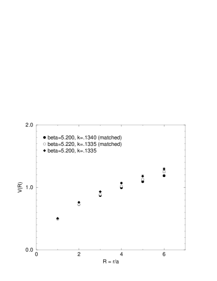
Figure 2: Static potential on an $8^{3}\times 24$ lattice at $(5.2,0.1340)$ and $(5.220,0.1335)$ where the average plaquette values match.

4 OTHER APPLICATIONS

The Lanczos quadrature technique allows one to build relatively efficient stochastic estimators (6) of the fermion determinant suitable for a variety of purposes including:

• matching observables (see above)

• tuning approximate actions [5]

• tuning exact algorithms based on these

• choosing parallel tempering ensembles [11].

In particular, a suitably truncated version may be used to model the low eigenmodes of the determinant [12] while using other gauge invariant operators (e.g. Wilson loops) [5] to account for the remainder. Preliminary tests [10] have demonstrated that relatively few Lanczos iterations are required to obtain a good quantitative account of the fermion determinant. Both the truncation parameters and the gauge loop parameters must be tuned, using the above techniques, to obtain a useful representation of the true QCD action and to ensure a good acceptance of configurations proposed by the gauge part of the update. Such approximate actions can of course be made exact via an accept/reject step, given sufficiently accurate tuning [5].

References

- [1] M. Talevi, UKQCD collaboration Nucl. Phys. B (Proc. Suppl.) 63A-C (1998) 227.
- [2] C. Allton et al, UKQCD collaboration, hep-lat/9808016.
- [3] M. Talevi, UKQCD collaboration, these proceedings.
- [4] R. Sommer, Nucl. Phys. B411 (1994) 839.
- [5] A. C. Irving and J. C. Sexton, Phys. Rev. D55 (1997) 5456.
- [6] A. C. Irving, J. C. Sexton and E. Cahill, Nucl. Phys. B (Proc. Suppl.) 63A-C (1998) 967
- [7] Z. Bai, M. Fahey and G. Golub, ‘Some Large Scale Matrix Computation Problems’, Technical report SCCM-95-09, School of Engineering, Stanford University (1995).
- [8] E. Cahill, J. C. Sexton and A. C. Irving, in preparation.
- [9] K. Jansen and R. Sommer, hep-lat/9709022.
- [10] A. C. Irving et al., hep-lat/9808015.
- [11] B. Joó, UKQCD collaboration, these proceedings.
- [12] A. Duncan, E. Eichten and H. Thacker, hep-lat/9806020.