Numerical simulation of dynamical gluinos: experience with a multi-bosonic algorithm and first results

Abstract

We report on our experience with the two-step multi-bosonic algorithm in a large scale Monte Carlo simulation of the SU(2) Yang-Mills theory with dynamical gluinos. First results are described on the low lying spectrum of bound states, the string tension and the gluino condensate.

1 INTRODUCTION

An important step towards the understanding of non-perturbative properties of supersymmetric (SUSY) gauge theories is the numerical simulation of the supersymmetric extension of Yang-Mills (SYM) theory. The theoretical motivation for this has been summarized at the previous [1] and present [2] lattice conferences. (For references see these reviews and [3].) First steps towards a numerical Monte Carlo simulation with dynamical gluinos have already been presented a year ago [4]. Since then our collaboration made important progress in a first large scale simulation of SU(2) SYM on the CRAY T3E-512 at HLRZ Jülich. This is a short status report which will be followed soon by a more detailed publication.

1.1 Lattice action

The SU(2) Yang-Mills theory with gluinos (= Majorana fermions in the triplet representation) becomes supersymmetric in the massless limit. Massive gluinos break SUSY softly. For a lattice regularization one can take the Wilson action for gauge field and gluinos, as proposed some time ago by Curci and Veneziano [5]. This contains two bare parameters: $\beta$ for the gauge coupling and $K$ for the hopping parameter (bare gluino mass). The Majorana nature of the gluino is taken into account by considering $N_{f}=\frac{1}{2}$ adjoint Dirac flavours. The effective action for the gauge field assumes the form

$$S_{CV}=\beta\sum_{pl}\left(1-\frac{1}{2}{\rm Tr\,}U_{pl}\right)-\frac{1}{2}\log\det Q[U]\ ,$$ (1)

where the fermion matrix is

$$Q_{yv,xu}=\delta_{yx}\delta_{vu}-K\sum_{\mu=\pm}\delta_{y,x+\hat{\mu}}(1+\gamma_{\mu})V_{vu,x\mu}$$ (2)

with the gauge link in the adjoint representation $V_{vu,x\mu}=\frac{1}{2}{\rm\,Tr\,}(U_{x\mu}^{\dagger}\tau_{v}U_{x\mu}\tau_{u})$.

An interesting new development is that an exactly zero mass gaugino can be described on the lattice by the Neuberger-action [6]. (Concerning chiral symmetry see [7].) The technical difficulty is to determine the necessary inverse square-root $(Q^{\dagger}Q)^{-\frac{1}{2}}$. For this we can use the quadratically optimized polynomials discussed in sec. 2. The results of a numerical study of the Neuberger-action will be published elsewhere.

1.2 Pfaffians

The Curci-Veneziano action assumes $\det(Q)^{\frac{1}{2}}$ for the Majorana fermion. This may lead to a sign problem because the path integral for Majorana fermions gives the Pfaffian

$${\rm Pf}(M)\equiv\int[d\phi]e^{-\frac{1}{2}\phi_{\alpha}M_{\alpha\beta}\phi_{\beta}}$$ (3)

$$= \frac{1}{N!2^{N}}\epsilon_{\alpha_{1}\beta_{1}\ldots\alpha_{N}\beta_{N}}M_{\alpha_{1}\beta_{1}}\ldots M_{\alpha_{N}\beta_{N}}\ ,$$

where $M\equiv CQ$ satisfies

$${\rm Pf}(M)^{2}=\det(M)=\det(Q)=\det(\tilde{Q})\ .$$ (4)

Here $\tilde{Q}\equiv\gamma_{5}Q$ is the hermitean fermion matrix. Since $\tilde{Q}$ has doubly degenerate real eigenvalues, the determinant is non-negative: $\det(Q)\geq 0$. The sign of the Pfaffian is, however, unknown.

A numerical procedure for the computation of Pfaffians can be based on the decomposition [8]

$$M=P^{T}JP,\hskip 20.00003pt{\rm Pf}(M)=\det(P)\ ,$$ (5)

where $J$ is a block-diagonal matrix containing on the diagonal $2\otimes 2$ blocks equal to $\epsilon=i\sigma_{2}$. This form of $M$ can be achieved by a procedure analogous to the Gram-Schmidt orthogonalization and then $P$ turns out to be a triangular matrix. (See e.g. the treatment of simplectic groups in [9].)

The numerical procedure requires the storage of a full $N\otimes N$ matrix, similarly to the determinant calculation by LU-decomposition. Therefore, one can only deal with relatively small lattices. In a test with dynamical gluino updating at $(\beta=2.3,K=0.1925)$ on $4^{3}\cdot 8$ lattice the Pfaffian of every randomly chosen configuration turned out to be positive (see fig. 1).

Figure 1: The values of the pfaffian on $4^{3}\cdot 8$ lattice at $(\beta=2.3,K=0.1925)$ versus the largest eigenvalue $\lambda_{max}$ of $Q^{\dagger}Q$.

In general, however, the Pfaffian is not always positive. In fact, if a pair of degenerate eigenvalues of the hermitean fermion matrix $\tilde{Q}$ changes sign, it is plausible that the sign of ${\rm Pf}(M)$ changes, too. An example is shown by fig. 2, where one of the configurations in fig. 1 is considered as a function of the “valence” hopping parameter $K_{v}$ in $M$. As the numerical determination of the nearly zero eigenvalues of $\tilde{Q}$ shows, at the same $K_{v}$ where ${\rm Pf}(M)$ changes sign there is also a sign change of an eigenvalue pair.

Figure 2: The absolute value of the pfaffian on a $4^{3}\cdot 8$ configuration as a function of the hopping parameter in $M$ (and $\tilde{Q}$). Open points stand for ${\rm Pf}(M)>0$, full ones for ${\rm Pf}(M)<0$.

The spectral flow of $\tilde{Q}$ is relevant for the overlap-inspired fermionic definition of the topological charge (see [10] and references therein). Since the index of a massless Dirac operator in the adjoint representation of SU(2) in a gauge field background of topological charge $Q_{top}$ is $4Q_{top}$ [11], this suggests that at the hopping parameter value $K^{\prime}$ used in the Neuberger action the sign of ${\rm Pf}(M)$ is given by

$${\rm Pf}(M(K^{\prime}))/|{\rm Pf}(M(K^{\prime}))|=e^{2\pi iQ_{top}}.\$$ (6)

One has to have in mind that the fermionic definition can also give half-integer topological charges. (For SU($N_{c}$) gauge theory the topological charge can be an integer multiple of $1/N_{c}$.) Since $K^{\prime}$ is larger than the dynamical hopping parameter $K$ and the level crossings typically occur between $K$ and $K^{\prime}$, it is plausible that the path integral at $K$ is dominated by configurations with positive Pfaffian. Therefore the Curci-Veneziano action gives the same continuum limit as the definition with the path integral over Majorana fermions.

The question of fractional topological charges is important for the low energy effective action [13] which assumes a remnant chiral symmetry $Z_{2N_{c}}$. In fact, if fractional topological charges would exist, the $\theta$-parameter would be periodic only with $2\pi N_{c}$ and the remnant chiral symmetry would be $Z_{2}$, instead of $Z_{2N_{c}}$. In this case the spontaneous symmetry breaking $Z_{2N_{c}}\to Z_{2}$ would be absent and there would be no first order phase transition at zero gluino mass. In the quenched continuum limit the half-integer topological charges seem to persist [12] but the continuum limit with dynamical gluinos may be different.

2 MULTI-BOSONIC ALGORITHM

The multi-bosonic algorithm for Monte Carlo simulations of fermions has been proposed by Lüscher [14]. In the original version for $N_{f}$ flavours one considers the approximation of the fermion determinant

$$\left|\det(Q)\right|^{N_{f}} = \left\{\det(Q^{\dagger}Q)\right\}^{N_{f}/2}$$ (7)

$$\simeq \frac{1}{\det P_{n}(Q^{\dagger}Q)}$$

where the polynomial $P_{n}$ satisfies

$$\lim_{n\to\infty}P_{n}(x)=x^{-N_{f}/2}$$ (8)

in an interval $[\epsilon,\lambda]$ covering the spectrum of $Q^{\dagger}Q$. For the multi-bosonic representation of the determinant one uses

$$P_{n}(Q^{\dagger}Q)=P_{n}(\tilde{Q}^{2})=r_{0}\prod_{j=1}^{n}(\tilde{Q}-\rho_{j}^{*})(\tilde{Q}-\rho_{j})$$ (9)

and then

$$\prod_{j=1}^{n}\det[(\tilde{Q}-\rho_{j}^{*})(\tilde{Q}-\rho_{j})]^{-1}\propto$$

$$\int[d\Phi]\exp\{-\sum_{j=1}^{n}\sum_{xy}\Phi_{jy}^{+}(\tilde{Q}-\rho_{j}^{*})(\tilde{Q}-\rho_{j})\Phi_{jx}\}$$ (10)

The difficulty for small fermion masses is that the condition number $\lambda/\epsilon$ becomes very large ($10^{4}-10^{6}$) and very high orders $n={\cal O}(10^{3})$ are required for a good approximation. This requires large storage and the autocorrelation becomes bad since it is proportional to $n$.

2.1 Improved version: two-step updating

Substantially smaller storage and shorter autocorrelations for small fermion masses can be achieved by starting from a two-step approximation [15]:

$$\left\{\det(Q^{\dagger}Q)\right\}^{N_{f}/2}$$

$$\;\simeq\;\frac{1}{\det P^{(1)}_{n_{1}}(Q^{\dagger}Q)\det P^{(2)}_{n_{2}}(Q^{\dagger}Q)}$$ (11)

where now

$$\lim_{n_{2}\to\infty}P^{(1)}_{n_{1}}(x)P^{(2)}_{n_{2}}(x)=x^{-N_{f}/2}\ ,\hskip 10.00002ptx\in[\epsilon,\lambda]\ .$$ (12)

The multi-bosonic representation of the determinant is used for $\det P^{(1)}_{n_{1}}$. The correction factor $\det P^{(2)}_{n_{2}}$ is realized in a noisy correction step [16] with the accept-reject function

$$e^{-\eta^{\dagger}\left\{P^{(2)}_{n_{2}}(\tilde{Q}[U^{\prime}]^{2})-P^{(2)}_{n_{2}}(\tilde{Q}[U]^{2})\right\}\eta}$$ (13)

where $\eta$ is generated from the simple Gaussian noise $\eta^{\prime}$ with a suitable polynomial approximation $P^{(3)}_{n_{3}}$ as

$$\eta=P^{(2)}_{n_{2}}(\tilde{Q}[U]^{2})^{-\frac{1}{2}}\eta^{\prime}\Rightarrow P^{(3)}_{n_{3}}(\tilde{Q}[U]^{2})\eta^{\prime}\ .$$ (14)

An important gain in performance is obtained by the use of quadratically (“least-square”) optimized polynomials [17]. The Chebyshev- (for $N_{f}=2$) or Legendre- (for $N_{f}=1$) polynomials are bad for large $\lambda/\epsilon$. The quadratically optimized polynomials are much better. Note that, as discussed in sec. 1.1, for gluinos one has to consider $N_{f}=\frac{1}{2}$.

A complete cycle of sweeps contains heatbath and overrelaxations sweeps for the boson fields and a Metropolis sweep for the gauge field followed by the accept-reject step. We choose the order of the first polynomial such that the acceptance rate in the accept-reject step is typically 80-90%. The longest autocorrelations appear for “gluonic” quantities depending on gauge field variables. For instance, in our runs the autocorrelation of the plaquette expectation value is typically given by $\tau_{int}^{plaq}\simeq 300-400$ cycles. The “fermionic” autocorrelations are about a factor $\simeq 10$ smaller.

2.2 Measurement correction

To avoid systematic errors, both in the original version and in the two-step version the polynomial approximations have to be taken, in principle, to infinite order. In praxis it is enough that the errors introduced by the polynomial approximations are smaller than the statistical errors. However, due to the limited approximation quality, for small fermion masses sometimes exceptional configurations with very small ($10^{-8}-10^{-10}$) eigenvalues of $Q^{\dagger}Q$ are generated. In order to avoid these one could increase the polynomial orders but it is more economical to perform a measurement correction step by a generalization of the method of ref. [18]. In this way the expectation value of a quantity $A$ is given by

$$\langle A\rangle=\frac{\langle A\exp{\{\eta^{\dagger}[1-P^{(4)}_{n_{4}}(Q^{\dagger}Q)]\eta\}}\rangle_{U,\eta}}{\langle\exp{\{\eta^{\dagger}[1-P^{(4)}_{n_{4}}(Q^{\dagger}Q)]\eta\}}\rangle_{U,\eta}}\ ,$$ (15)

where $\eta$ is a Gaussian noise and the polynomial $P^{(4)}_{n_{4}}$ is such that $P^{(1)}_{n_{1}}P^{(2)}_{n_{2}}P^{(4)}_{n_{4}}$ is an optimized approximation of the function $x^{-N_{f}/2}$ in the interval $[\epsilon^{\prime},\lambda]$. This correction step can be arranged in such a way that one obtains an “exact” algorithm. For instance, $\epsilon^{\prime}$ can be set to zero and then the correction step is not sensitive to the fluctuations of the smallest eigenvalue. (Note that in our case the least-square optimization can also be achieved for zero lower boundary of the interval, in contrast e.g. to the minimization of the maximal relative deviation with Chebyshev polynomials.) For the evaluation of $P^{(4)}_{n_{4}}$ one can use $n_{4}$-independent recursive relations [17] which can be stopped by observing the convergence of the result. Another possibility is to take $\epsilon^{\prime}>0$ and to perform the correction exactly for the few exceptional eigenvalues below $\epsilon^{\prime}$ by multiplying with $\lambda^{N_{f}/2}P^{(1)}_{n_{1}}(\lambda)P^{(2)}_{n_{2}}(\lambda)$.

Experience shows that for most physical quantities the exceptional configurations give no exceptional contributions. There are, however, also some quantities which are sensitive to the small eigenvalues, hence the measurement correction is essential (see fig. 3).

Figure 3: The measurement correction for the a-pion propagator at zero distance. The exceptional configurations with small eigenvalues contribute strongly to the raw data. After correction these contributions are still important but of normal size.

As the figure shows, even the small lower limit of the polynomial approximation interval $\epsilon=10^{-5}$, in connection with the polynomial orders $n_{1}=24,\;n_{2}=200$, is insufficient for suppressing the exceptional configurations. In this case a measurement correction step with $\epsilon^{\prime}=0$ and $n_{4}=400$ is enough for good precision.

3 APPROACHING
SUPERSYMMETRY

The Monte Carlo simulations have been performed up to now mainly at $\beta=2.3$. After last years tests at lower hopping parameter values [4] we are presently concentrating on the interval $0.185\leq K\leq 0.1975$. Lattice sizes range from $4^{3}\cdot 8$ to $12^{3}\cdot 24$. The characteristic feature of these simulations are the rather large condition numbers growing up to $\lambda/\epsilon=10^{5}-10^{6}$. Our present best estimate for the critical hopping parameter for zero gluino mass is $K_{0}\simeq 0.195$ (see sec. 3.3). This means that the bare gluino mass in lattice units at e.g. $K=0.1925$ is about $am_{0}\equiv\frac{1}{2}(K_{0}^{-1}-K^{-1})\simeq 0.03$. This gives a ratio to the smallest glueball mass $m_{0}/M^{0^{+}}\simeq 0.08$. The large condition numbers are further increased if the “valence” hopping parameter $K_{v}$ in the gluino propagators is increased. A typical example for the average of the lowest eigenvalue is shown in fig. 4.

Figure 4: The average lowest eigenvalue of $Q^{\dagger}Q$ as a function of the inverse (valence) hopping parameter in a dynamical update at ($\beta=2.3,K=0.1925$) on $8^{3}\cdot 16$ lattice. The error bars here show standard deviations (not the errors of averages).

(The approximation interval for polynomials is in this case $[\epsilon,\lambda]=[0.0001,3.7]$.) As one can see, near $1/K_{v}=1/0.2025\simeq 4.94$ the average smallest eigenvalue becomes rather small and fluctuates practically down to zero. For smaller values of $1/K_{v}$ the picture remains unchanged. This agrees with the findings of ref. [10] about the absence of the spectrum gap for a range of bare fermion masses. (Note that the start of the gapless region at $K_{v}=0.2025$ lies higher than $K_{0}$ because in fig. 4 the dynamical “sea” gluino mass is not changing.)

3.1 Bound state masses

A basic assumption about the dynamics of SYM theory is that there is confinement. The colourless bound states should be organized in degenerate supermultiplets which are split up at non-zero gluino mass. The pattern of states should be similar to QCD with a single flavour of quarks. For instance, the low-lying meson states have quantum numbers as $\eta^{\prime},\;f_{0}$ etc. Since our constituent gluinos are in the adjoint representation, we call these states $a$-$\eta^{\prime},\;a$-$f_{0}$ etc. There are, of course, also the glueball states ($gg$) as in pure gauge theory and for completing the supermultiplets we also need spin-$\frac{1}{2}$ states: the gluino-glueballs ($\tilde{g}g$).

We determine the masses of low-lying states by using the blocking-smearing technology for achieving better projections to the sources and sinks. Our preliminary results are summarized in fig. 5.

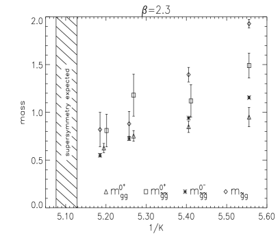
Figure 5: The preliminary results for bound state masses.

The presence of two distinct light $0^{+}$ states in the spectrum seems to prefer the generalization of the Veneziano-Yankielowicz action [13] proposed in ref. [19].

3.2 String tension

Figure 6: The three-parameter fit to the static potential: $V(R)=V_{0}+\sigma R-\alpha/R$ at ($\beta=2.3,K=0.19$) on $8^{3}\cdot 16$ lattice.

The confinement can be characterized by the string tension obtained from the linear part of the static potential at large distances. We determined the static potential from APE-smeared Wilson loops following [20]. At ($\beta=2.3,K=0.19$) on $8^{3}\cdot 16$ lattice the optimized smearing radius is 3.3 and we obtained stable results against variations of the $T$ fit-interval. As shown by fig. 6, the result for the square root of the string tension in lattice units is $a\sqrt{\sigma}=0.21(1)$. At $K=0.1925$ the corresponding value is surprisingly small: $a\sqrt{\sigma}=0.10(3)$ but the $8^{3}\cdot 16$ lattice might be too small in this case, causing finite volume effects.

3.3 Gluino condensate

If there are no fractional topological charges, the hopping parameter $K_{0}$ corresponding to zero gluino mass is signaled by a first order phase transition which is due to the spontaneous discrete chiral symmetry breaking $Z_{4}\to Z_{2}$. The gluino condensate should have a jump of order ${\cal O}(1)$ in lattice units [3]. It is possible that this transition develops only in the continuum limit and at finite lattice spacings it shows up just as a fast cross-over. Our preliminary results are summarized in fig. 7. The jump at $1/K=1/0.195\simeq 5.13$ suggests a vanishing gluino mass at $K_{0}\simeq 0.195$.

Figure 7: The preliminary results for the gluino condensate.

Acknowledgements: It is a pleasure to thank Gernot Münster for helpful discussions. J. Westphalen acknowledges the financial contribution of the European Commission under the TMR-Program ERBFMRX-CT97-0122.

References

- [1] I. Montvay, Nucl. Phys. Proc. Suppl. 63 (1998) 108.
- [2] M.J. Strassler, this Proceedings.
- [3] I. Montvay, hep-lat/9801023.
- [4] G. Koutsoumbas, I. Montvay, A. Pap, K. Spanderen, D. Talkenberger, J. Westphalen, Nucl. Phys. Proc. Suppl. 63 (1998) 727.
- [5] G. Curci and G. Veneziano, Nucl. Phys. B292 (1987) 555.
- [6] H. Neuberger, Phys. Lett. B417 (1998) 141; Phys. Rev. D57 (1998) 5417.
- [7] F. Niedermayer, this Proceedings.
- [8] N. Bourbaki, Algèbre, Chap. IX., Hermann, Paris, 1959.
- [9] M. Hamermesh, Group Theory and its Applications to Physical Problems, Adison-Wesley, Reading, 1962.
- [10] R.G. Edwards, U.M. Heller, R. Narayanan, hep-lat/9802016.
- [11] T. Eguchi, P.B. Gilkey, A.J. Hanson, Phys. Rep. 66 (1980) 213.
- [12] R.G. Edwards, U.M. Heller, R. Narayanan, hep-lat/9806011.
- [13] G. Veneziano, S. Yankielowicz, Phys. Lett. B113 (1982) 231.
- [14] M. Lüscher, Nucl. Phys. B418 (1994) 637.
- [15] I. Montvay, Nucl. Phys. B466 (1996) 259.
- [16] A.D. Kennedy, J. Kuti, Phys. Rev. Lett. 54 (1985) 2473.
- [17] I. Montvay, Comput. Phys. Commun. 109 (1998) 144.
- [18] R. Frezzotti, K. Jansen, Phys. Lett. B402 (1997) 328.
- [19] G.R. Farrar, G. Gabadadze, M. Schwetz, hep-th/9711166, hep-th/9806204.
- [20] G.S. Bali, K. Schilling, Ch. Schlichter, Phys. Rev. D51 (1995) 5165.