The spectral dimension of non-generic branched polymers

Abstract

We show that the spectral dimension on non-generic branched polymers with susceptibility exponent $\gamma>0$ is given by $d_{s}=2/(1+\gamma)$. For those models with $\gamma<0$ we find that $d_{s}=2$.

1 INTRODUCTION

The manifolds in the ensemble of two-dimensional quantum gravity have a rich structure which can be characterized in a number of different ways. In particular there are several different quantities which in the case of smooth regular manifolds take the same value and correspond to the usual notion of dimension. When computed for manifolds which are far from regular these quantities, which in fact probe different aspects of the geometry, can yield different values.

The Hausdorff dimension $d_{h}$ is defined through the volume, $dV$ of an annulus of geodesic thickness $dR$ at geodesic distance $R$ from a point by

$$dV\sim R^{d_{h}-1}\,dR$$ (1)

On the other hand the spectral dimension $d_{s}$ describes the properties of a random walk, generated by the diffusion equation, on the manifold. A walker sets off from a point P; the probability that after making $t$ steps (a step is defined as a move from one lattice point to a neighbouring one in discretized quantum gravity) he has returned to P is

$$P(t)\sim\frac{1}{t^{d_{s}/2}}$$ (2)

provided that $N^{\Delta}\gg t\gg 1$ to avoid finite size and discretization effects respectively. For smooth regular two dimensional manifolds $d_{h}=d_{s}=2$. The spectral dimension has been determined for various two-dimensional quantum gravity systems by Monte Carlo simulation, scaling relations, and exact calculation. In [1] it was shown that for the generic branched polymer ensemble $d_{s}=4/3$ whereas the corresponding Hausdorff dimension is 2 [3]. Using the same method we have now extended the calculation to the non-generic branched polymers [2].

2 CALCULATION

The branched polymer ensembles have a grand canonical partition function $Z(\mu)$ given by [3]

$$Z(\mu)=e^{-\mu}(1+\sum_{n=1}^{\infty}\alpha_{n}Z(\mu)^{n})$$ (3)

which is non-analytic as $\mu\downarrow\mu_{cr}$ with behaviour

$$Z(\mu)\simeq Const-(\mu-\mu_{cr})^{1-\gamma}$$ (4)

For generic branched polymers (a finite number of $\alpha_{n}$ non-zero, and all positive) we get $\gamma=1/2$; the multi-critical BPs (at least $k$ $\alpha$s non-zero and specially tuned) have $\gamma=1-1/(k+1)$ with $k=2,3,\ldots$ and the continuous critical BPs have any $\gamma<1$ at the expense of having an infinite number of the $\alpha$s non-zero.

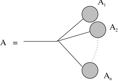
Figure 1: The constituents ${\rm A}_{1},\ldots,{\rm A}_{n}$ of a branched polymer $\rm A$.

Our calculation of $d_{s}$ for the non-generic BPs [2] follows the method of [1]; the main generalization is that the generating function for the return probabilities on any branched polymer A can always be expressed in terms of those for its constituents ${\rm A}_{1},{\rm A}_{2},\ldots$ (see fig.1). Letting

$$P_{{\rm A}}(y)=\sum_{t}y^{t}P(t)=\frac{1}{1-y}\frac{1}{h_{{\rm A}}(y)}$$ (5)

we find that

$$h_{{\rm A}}(y)=\frac{1+\sum_{i=1}^{n}h_{{\rm A}_{i}}(y)}{1+(1-y)\sum_{i=1}^{n}h_{{\rm A}_{i}}(y)}$$ (6)

The main result that we prove is that defining

$$H_{{\rm A}}^{(n_{1},n_{2},\ldots,n_{p})}=\prod_{i=1}^{p}\frac{d^{n_{i}}}{dy^{n_{i}}}h_{{\rm A}}(y)|_{y=1}$$ (7)

then

$$H^{(n_{1},n_{2},\ldots,n_{p})}(z)=\sum_{{\rm A}}z^{N_{{\rm A}}}w_{{\rm A}}H_{{\rm A}}^{(n_{1},n_{2},\ldots,n_{p})}$$ (8)

has the asymptotic behaviour

$$H^{(n_{1},n_{2},\ldots,n_{p})}(z)\sim(z_{cr}-z)^{1-\gamma-p-(1+\gamma)\sum_{i=1}^{p}n_{i}}$$ (9)

(where $z=e^{-\mu}$, the sum over A runs over all BPs, $N_{{\rm A}}$ is the number of links in A, and $w_{{\rm A}}$ the weight for A in the graphical expansion of (3)). This is done by induction on $n$ and $p$ and using (6) to generate the derivatives.

Using this result we can compute the asymptotic expansion of the grand canonical generating function

$${\cal P}(z,y)=\sum_{{\rm A}}z^{N_{{\rm A}}}w_{{\rm A}}P_{{\rm A}}(y)$$ (10)

Taking the n’th derivative of (10) and setting $y=1$ yields a sum of terms which are precisely the $H^{(n_{1},n_{2},\ldots,n_{p})}(z)$. Thus we are able to show that (supposing for a moment that the Taylor series is convergent about $y=1$, and dropping a trivial pole term)

$${\cal P}(z,y)=\left(1-z/z_{cr}\right)^{\beta}\Phi\left(\frac{1-y}{\left(1-z/z_{cr}\right)^{\Delta}}\right)$$ (11)

with $\beta=1-2\gamma$ and $\Delta=1+\gamma$. In fact the Taylor series is not convergent, nor is it Borel summable. However it is possible to prove [1] that it is an asymptotic series with an integral representation which has no unphysical singularities in the region of interest. The absence of Borel summability means that this integral representation is not unique; however it can only differ from the true result by terms involving essential singularities which vanish at $y=1$. Since $\cal P$ has ordinary non-analytic behaviour at $y=1$ these possible essential singularities can have no effect on the physics.

3 RESULTS

It was shown in [2] that the critical behaviour of $\cal P$ is related to the spectral dimension through

$$\beta=1-\gamma+\Delta\left(\frac{d_{s}}{2}-1\right)$$ (12)

When $\gamma>0$ we find that $d_{s}=2/(1+\gamma)$. This is of course consistent with the previously known result for the generic case. It also shows that the spectral dimension is not an independent critical exponent for these models – it is completely determined by $\gamma$. For the models with $\gamma<0$ (for which $\Delta=1$ and $\beta=1-\gamma$) we find that $d_{s}=2$ always. This is the same as the value now established for the quantum gravity phase [4] but this is a coincidence. The negative $\gamma$ BPs are rather pathological objects being very bushy (this is the effect of the dominance of the high order branching in (3)) and there is no sense in which the walker is really “diffusing”; in reality he is just going backwards and forwards along the short branches of the bush. One cannot deduce from the coincidence of $d_{s}$ that negative $\gamma$ BPs are the same as the quantum gravity phase!

References

- [1] T.Jonsson, J.F.Wheater, Nucl. Phys. B 515 (1998) 549.
- [2] J.D.Correia, J.F.Wheater, Phys. Lett. B 422 (1998) 76.
- [3] J.Ambjørn, B.Durhuus, T.Jonsson, Phys. Lett. B 244 (1990) 403.
- [4] J. Ambjorn, D. Boulatov, J.L. Nielsen, J. Rolf, Y. Watabiki, J.High Energy Phys. 02 (1998) 010.