Oxford Preprint OUTP–98–53–P

Edinburgh Preprint 98/11

Liverpool Preprint LTH 430

Swansea Preprint SWAT 196

Light hadron spectroscopy with $O(a)$ improved dynamical fermions
UKQCD Collaboration

C.R. Allton¹, S.P. Booth², K.C. Bowler³, M. Foster⁴, J. Garden³, A.C. Irving⁴, R.D. Kenway³, C. Michael⁴, J. Peisa⁴, S.M. Pickles³, J.C. Sexton⁵, Z. Sroczynski³, M. Talevi³, H. Wittig⁶

¹ Department of Physics, University of Wales, Singleton Park, Swansea SA2 8PP, UK

² Edinburgh Parallel Computing Centre, University of Edinburgh, Edinburgh EH9 3JZ, Scotland

³ Department of Physics & Astronomy, University of Edinburgh, Edinburgh EH9 3JZ, Scotland

⁴ Division of Theoretical Physics, Department of Mathematical Sciences, University of Liverpool, Liverpool L69 3BX, UK

⁵ School of Mathematics, Trinity College, Dublin 2, and Hitachi Dublin Laboratory, Dublin 2, Ireland

⁶ Theoretical Physics, University of Oxford, Oxford OX1 3NP, UK

We present the first results for the static quark potential and the light hadron spectrum using dynamical fermions at $\beta=5.2$ using an $O(a)$ improved Wilson fermion action together with the standard Wilson plaquette action for the gauge part. Sea quark masses were chosen such that the pseudoscalar-vector mass ratio, $m_{\rm PS}/m_{\rm V}$, varies from $0.86$ to $0.67$. Finite-size effects are studied by using three different volumes, $8^{3}\cdot 24,12^{3}\cdot 24$ and $16^{3}\cdot 24$. Comparing our results to previous ones obtained using the quenched approximation, we find evidence for sea quark effects in quantities like the static quark potential and the vector-pseudoscalar hyperfine splitting.

1 Introduction

Recent years have seen a lot of progress in understanding the spectrum and the decays of hadrons using numerical simulations of lattice QCD (for recent reviews see [1, 2, 3]). While much effort has been invested in controlling systematic errors such as finite-size effects and lattice artefacts, the inclusion of quark loops in the stochastic evaluation of the Feynman path integral still presents a major challenge. Therefore, most simulations rely on the quenched approximation for which the systematic errors incurred by neglecting dynamical quark effects cannot be assessed. However, recent progress in the development of efficient algorithms [4] and increased computer power, has greatly increased the prospects for simulations with dynamical quarks. Several groups have published results for hadronic quantities in the light quark sector and the static quark potential from dynamical simulations [5, 6, 7, 8, 9, 10, 11, 12]. At the same time it has been demonstrated that leading lattice artefacts of order $a$ in physical observables can be eliminated through the non-perturbative implementation of the Symanzik improvement programme [13, 14]. The non-perturbatively $O(a)$ improved Wilson action has been determined in the quenched approximation [15, 16], and first results have also been reported for $n_{f}=2$ flavours of dynamical quarks [17]. This enables one to study the effects of the inclusion of dynamical quarks whilst having better control over discretisation errors.

In this work we report on calculations of the light hadron spectrum using two flavours of $O(a)$-improved dynamical Wilson quarks at $\beta=5.2$. For the improvement (clover) coefficient we have used $c_{\rm sw}=1.76$, a preliminary estimate kindly supplied by the Alpha Collaboration prior to the final result $c_{\rm sw}=2.017$ at $\beta=5.2$, presented in [17]. The main aim of this study is to understand qualitative features of dynamical simulations with improved fermions, such as the sea quark mass dependence of observables, finite-volume effects and estimates of autocorrelation times. The complete removal of $O(a)$ lattice artefacts is therefore not our highest priority in this work. Results for the hadron spectrum obtained with the “correct” values of $c_{\rm sw}$ will be published elsewhere [18].

The plan for the remainder of this paper is as follows. In section 2 we describe the details of our simulation, including the implementation of the algorithm and the analysis of autocorrelations. Section 3 contains our results for the static quark potential. The results for the light hadron spectrum and discussions of finite-volume and sea quark effects are presented in section 4. Section 5 contains our conclusions. Finally, in Appendix A we list our results for hadron masses on all lattice sizes and parameter values.

2 The simulation

In this section we fix our notation, describe the details of the implementation of the Generalised Hybrid Monte Carlo (GHMC) algorithm [19] on the Cray T3E, and give an overview of the simulation parameters used in our calculation. We end this section with a discussion of autocorrelations.

2.1 Lattice action

The lattice action can be split into a pure gauge part $S_{G}$ and a fermionic part $S_{F}$

$$S[U,\overline{\psi},\psi]=S_{G}[U]+S_{F}[U,\overline{\psi},\psi],$$ (1)

where

$$S_{G}[U]=\beta\sum_{P}\left(1-\frac{1}{3}{\rm Re\,Tr\,}U_{P}\right)$$ (2)

is the Wilson plaquette action, and $S_{F}$ is defined by

$$S_{F}[U,\overline{\psi},\psi]=S_{F}^{W}[U,\overline{\psi},\psi]-c_{\rm sw}\frac{i\kappa}{2}\sum_{x,\mu,\nu}\overline{\psi}(x)\sigma_{\mu\nu}F_{\mu\nu}(x)\psi(x).$$ (3)

Here, $S_{F}^{W}$ is the standard Wilson action, and $c_{\rm sw}$ denotes the improvement coefficient multiplying the Sheikholeslami-Wohlert term [20]. The bare parameters of the theory are the gauge coupling $\beta\equiv 6/g_{0}^{2}$ and the hopping parameter $\kappa$. Here we work with a doublet of degenerate dynamical Wilson quarks, and hence gauge configurations are characterised by the set of parameters $(\beta,\kappa;c_{\rm sw})$. For a description of the GHMC algorithm it is useful to rewrite the fermionic part of the action in terms of a complex, bosonic pseudofermion field $\phi$. In matrix notation we have

$$S_{F}=\phi^{\dagger}\left(M^{\dagger}M\right)^{-1}\phi-2\sum_{\rm even~{}sites}\,\ln\det\,A_{xx}.$$ (4)

The odd-even preconditioned fermion matrix $M$ is given by

$$M_{xy}=A_{xx}-\kappa^{2}D_{xz}A_{zz}^{-1}D_{zy},$$ (5)

where $D$ is the Wilson-Dirac matrix and $A$ denotes the matrix for the Sheikholeslami-Wohlert term.

2.2 Implementation of the GHMC algorithm

The main limitation of the performance of the Cray T3E is the memory bandwidth. The increased complexity of the memory system and the fact that the processors support multiple instruction issue leads to a loss of performance even for highly optimised Fortran code. We have therefore chosen to write key routines in assembler, whilst using Fortran 90 for less CPU-intensive parts. Less than 25% of the required run time is spent executing Fortran code.

Using 32-bit instead of 64-bit precision to represent the fields increases the speed by a factor 1.7. However, this gain has to be weighed against the degradation of the acceptance rate, reversibility, and the accuracy in the evaluation of the (global) energy difference required in the Metropolis accept/reject step. The last issue has been addressed by evaluating energy differences site by site and performing the subsequent summation in higher precision.

The inversion of the fermion matrix was performed using the Stabilised Biconjugate Gradient (BiCGStab) algorithm with odd-even preconditioning [21]. The gain compared to using the ordinary Conjugate Gradient algorithm was 40%. Further algorithmic improvements applied in this simulation are described in [22].

The version of the Cray T3E used in this work consisted of 96 processors, each capable of 900 MFlops peak speed. Using all our algorithmic improvements and exploiting the architectural features of the T3E we typically achieve sustained speeds of 25–30 GFlops on such a configuration.

We now describe the integration schemes used in the molecular dynamics part of the GHMC algorithm. As usual one introduces a set of conjugate momenta $P$ for the gauge fields $U$. The HMC Hamiltonian is then defined as

$${\cal H}=T[P]+S_{G}[U]+S_{F}[U,\phi^{\dagger},\phi],$$ (6)

where $T[P]$ is the kinetic energy, and we have written $S_{F}$ in terms of pseudofermion fields $\phi$ and $\phi^{\dagger}$. $T[P]$ is related to the evolution operator ${\cal T}$ in molecular dynamics time $\tau$, so that for any given set $U$ and $P$ of gauge fields and conjugate momenta, respectively [23]

$${\cal T}=\left(\begin{array}[]{c}T_{P}\\ T_{U}\end{array}\right):\quad\left(\begin{array}[]{c}U(\tau)\\ P(\tau)\end{array}\right)\longrightarrow\left(\begin{array}[]{c}U(\tau+d\tau)\\ P(\tau+d\tau)\end{array}\right),$$ (7)

where $d\tau$ denotes a finite interval in simulation time. The operators $T_{P}$ and $T_{U}$ are defined by

$$T_{P}(d\tau) : U\longrightarrow e^{id\tau P}\,U$$

$$T_{U}(d\tau) : P\longrightarrow P-id\tau\frac{\partial}{\partial U}\left(S_{G}+S_{F}\right).$$ (8)

Since ${\cal T}$ represents a numerical integration of the equations of motion it does not conserve ${\cal H}$ but introduces an error $\Delta{\cal H}$. For a single application of ${\cal T}$ this error is expected to grow as a power of the timestep $d\tau$ [24, 25]

$$\Delta{\cal H}\propto(d\tau)^{q}.$$ (9)

Verification of this relation for a given integration scheme provides a check for the correct implementation of the equations of motion. We have compared three integration schemes defined by

$$T_{1} = T_{P}(d\tau)\,T_{U}(d\tau)$$ (10)

$$T_{2} = T_{P}(\frac{d\tau}{2})\,T_{U}(d\tau)\,T_{P}(\frac{d\tau}{2})$$ (11)

$$T_{3} = T_{P}(\frac{a}{2}d\tau)\,T_{U}(ad\tau)\,T_{P}(\frac{a+b}{2}d\tau)\,T_{U}(bd\tau)\,T_{P}(\frac{a+b}{2}d\tau)\,T_{U}(ad\tau)\,T_{P}(\frac{a}{2}d\tau),$$ (12)

where $a=1/(2-2^{1/3})$ and $b=-2^{1/3}/(2-2^{1/3})$. Note that $T_{2}$ is the standard leapfrog integration scheme. One expects that $T_{1},\,T_{2}$ and $T_{3}$ cause $\Delta{\cal H}$ to vary as $(d\tau)^{2}$, $(d\tau)^{3}$ and $(d\tau)^{5}$, respectively. This can be compared to the values of $q$ obtained from the slope of $\ln\Delta{\cal H}$ as a function of $\ln(d\tau)$. Such a comparison is shown in Table 1. The numerically determined values of $q$ agree well with the expected behaviour of $\Delta{\cal H}$ for the three integration schemes, and thus we conclude that the integration of the equations of motion has been implemented correctly. In our production runs we have chosen an integration scheme which, like $T_{2}$, is exact up to order $(d\tau)^{3}$. To this end we define the operators

$$T_{G}(d\tau) : P\longrightarrow P-id\tau\frac{\partial}{\partial U}S_{G}$$

$$T_{F}(d\tau) : P\longrightarrow P-id\tau\frac{\partial}{\partial U}S_{F},$$ (13)

and consider the generalised leapfrog integration scheme

$$T(d\tau)=T_{F}(\frac{d\tau}{2})\left[T_{G}(\frac{d\tau}{2n})T_{P}(\frac{d\tau}{n})T_{G}(\frac{d\tau}{2n})\right]^{n}T_{F}(\frac{d\tau}{2}).$$ (14)

This particular scheme allows for a more efficient evaluation of the derivative of $S_{G}+S_{F}$ with respect to the gauge field. It reduces to the simple leapfrog scheme for $n=1$. In practice, we have used $n=1$ or 2.

Finally we note that although the Generalised Hybrid Monte Carlo (GHMC) algorithm had been implemented, we have used standard Hybrid Monte Carlo (HMC) in all production runs.

scheme	$(d\tau)^{q}$	$q$
$T_{1}$	$(d\tau)^{2}$	1.982(4)
$T_{2}$	$(d\tau)^{3}$	3.053(2)
$T_{3}$	$(d\tau)^{5}$	5.056(6)

Table 1: The leading variation of $\Delta{\cal H}$ for the three integration schemes considered and measured values of $q$.

2.3 Simulation parameters

Our simulations have been performed at $\beta=5.2$. In order to be able to study consistently finite-volume effects and the dependence on the dynamical quark mass, we have used $c_{\rm sw}=1.76$ in all calculations described in this paper. The standard lattice size in this simulation was $12^{3}\cdot 24$ and was chosen such as to guarantee a spatial volume in physical units of more than $(1\,{\rm fm})^{3}$. Smaller and larger lattices of size $8^{3}\cdot 24$ and $16^{3}\cdot 24$ were used to monitor finite-size effects.

In order to distinguish the bare quark mass used in the generation of dynamical configurations from that used to compute quark propagators for hadronic observables, we introduce the notation $\kappa^{\rm sea}$ to denote the hopping parameter of the doublet of dynamical quarks, whilst reserving $\kappa^{\rm val}$ for the valence quarks. In order to study the dependence of observables on the sea quark mass, gauge configurations have been generated at several values of $\kappa^{\rm sea}$. In Table 2 we list lattice sizes, the values of $\kappa^{\rm sea}$ and $\kappa^{\rm val}$ and the number of configurations.

$L^{3}\cdot T$	$\beta$	$c_{\rm sw}$	#conf.	$\kappa^{\rm sea}$	$\kappa^{\rm val}$
$8^{3}\cdot 24$	5.2	1.76	78	0.1370	0.	1370	0.	1380	0.	1390	0.	1395
			100	0.1380	0.	1370	0.	1380	0.	1390	0.	1395
			100	0.1390	0.	1370	0.	1380	0.	1390	0.	1395
			60	0.1395	0.	1370	0.	1380	0.	1390	0.	1395
$12^{3}\cdot 24$	5.2	1.76	151	0.1370	0.	1370	0.	1380	0.	1390	0.	1395
			151	0.1380	0.	1370	0.	1380	0.	1390	0.	1395
			151	0.1390	0.	1370	0.	1380	0.	1390	0.	1395
			121	0.1395	0.	1370	0.	1380	0.	1390	0.	1395
			98	0.1398			0.	1380	0.	1390	0.	1395	0.	1398
$16^{3}\cdot 24$	5.2	1.76	90	0.1390					0.	1390	0.	1395	0.	1398
			100	0.1395					0.	1390	0.	1395	0.	1398
			69	0.1398					0.	1390	0.	1395	0.	1398

Table 2: Summary of simulation parameters and statistics for the computation of hadronic observables.

Quark propagators were calculated for every combination of $(\mbox{$\kappa^{\rm sea}$},\,\mbox{$\kappa^{\rm val}$})$ and combined to form hadronic two-point correlation functions. In order to increase the projection onto the ground state, the quark propagators used to form hadronic two-point functions have been “fuzzed” at the source and/or sink according to the prescription defined in [26]. Statistical errors of observables have been estimated using the bootstrap procedure described in [27] using 250 bootstrap samples.

2.4 Autocorrelations

The determination of autocorrelation times is important in order to achieve small statistical correlations among the ensemble of configurations and to eliminate the effects of insufficient thermalisation.

The autocovariance of an observable $\Omega$ is defined as [28]

$$\Gamma_{\Omega}(t)=\left\langle\left(\Omega_{s}-\langle\Omega\rangle\right)\left(\Omega_{s+t}-\langle\Omega\rangle\right)\right\rangle,$$ (15)

where the subscripts on $\Omega$ label the the values obtained on successive configurations. In practice, the expectation value $\langle\ldots\rangle$ is replaced by the ensemble average over a finite number of configurations. We define the autocorrelation function of $\Omega$ by

$$\rho_{\Omega}(t)=\Gamma_{\Omega}(t)/\Gamma_{\Omega}(0),$$ (16)

and from the large-$t$ behaviour of $\rho_{\Omega}$ one obtains the exponential autocorrelation time $\tau^{\rm exp}$

$$\rho_{\Omega}(t)\propto{\rm e}^{-t/\tau^{\rm exp}},\qquad t\to\infty.$$ (17)

The slowest mode of $\rho_{\Omega}$ is thus characterised by $\tau^{\rm exp}$, which is relevant for the equilibration of the system. By contrast, the integrated autocorrelation time $\tau^{\rm int}_{\Omega}$ depends on the observable and is required for the estimation of the statistical error in $\Omega$, once the system is in equilibrium. It is defined by

$$\tau^{\rm int}_{\Omega}=\frac{1}{2}\sum_{-\infty}^{\infty}\,\rho_{\Omega}(t)=\frac{1}{2}+\sum_{t=1}^{\infty}\,\rho_{\Omega}(t),$$ (18)

where the latter equality holds since $\rho_{\Omega}(-t)=\rho_{\Omega}(t)$. This definition implies that statistically independent configurations for quantity $\Omega$ are separated by $2\tau^{\rm int}_{\Omega}$. In practice one has to truncate the infinite sum in eq. (18) at some finite value $t_{\rm max}$. The resulting, so-called cumulative autocorrelation time $\tau^{\rm cum}_{\Omega}$

$$\tau^{\rm cum}_{\Omega}=\frac{1}{2}+\sum_{t=1}^{t_{\rm max}}\,\rho_{\Omega}(t)$$ (19)

is a good approximation to $\tau^{\rm int}_{\Omega}$, provided that $t_{\rm max}$ has been chosen large enough so that any further increase does not lead to an increase in $\tau^{\rm cum}_{\Omega}$. In other words, a plot of $\tau^{\rm cum}_{\Omega}$ versus $t_{\rm max}$ should ideally exhibit a plateau for large enough $t_{\rm max}$.

In order to obtain reliable estimates for $\tau^{\rm exp}$ and $\tau^{\rm cum}_{\Omega}$, autocorrelations should ideally be measured using ensembles containing many more configurations than the value of $\tau^{\rm int}_{\Omega}$. This requirement is not easy to satisfy in simulations whose primary aim is to compute hadronic properties, i.e. for which the calculation of observables requires a non-negligible amount of CPU time. A convenient quantity to determine autocorrelations is the average plaquette, which in our simulations has been measured after every HMC update, and not only on the subset of configurations used to compute quark propagators. Although $\tau^{\rm cum}_{\Omega}$ depends on the quantity $\Omega$, the integrated autocorrelation times estimated from the plaquette provide a useful guideline for the computation of hadronic observables.

Examples of our analysis of autocorrelations are shown in Fig. 1. Here, the statistical errors plotted for $\rho(t)$ and $\tau^{\rm cum}$ were estimated using a jackknife procedure. In order to take into account the effects of autocorrelations in the error estimate of $\rho(t)$ and $\tau^{\rm cum}$ themselves, the original data for these quantities were grouped in bins of size $h$. Jackknife averages were then formed for varying bin size, and by increasing $h$ until the jackknife errors stabilised, the error bands in the plots were obtained. Fig. 1 (a) shows a plot of $\ln\rho(t)$ versus $t$. $\tau^{\rm exp}$ and its error are extracted from the linear slope at large $t$ using a fitting routine. Fig. 1 (b) shows the cumulative autocorrelation time. The central value of $\tau^{\rm cum}$ and the error are read off in the region where $\tau^{\rm cum}$ shows no significant variation within statistical errors.

Figure 1: Autocorrelations for the average plaquette on $12^{3}\cdot 24$ and $\mbox{$\kappa^{\rm sea}$}=0.1370$. (a): $\ln\rho(t)$ plotted versus $t$; (b): the cumulative autocorrelation time plotted against $t_{\rm max}$ (see eq. (19)). The solid lines follow the computed values for $\ln\rho(t)$ and $\tau^{\rm cum}$. The dashed lines represent the error bands estimated from a jackknife procedure as described in the text.

Our results for $\tau^{\rm exp}$ and $\tau^{\rm cum}$ estimated from the average plaquette are shown in Table 3. One observes a pronounced dependence of autocorrelation times with the mass of the sea quark. In the range of $\kappa^{\rm sea}$ investigated in our study, $\tau^{\rm exp}$ and $\tau^{\rm cum}$ increase by roughly a factor of two as one goes to smaller sea quark masses. Also, a mild volume dependence of $\tau^{\rm exp}$ and $\tau^{\rm cum}$ is observed, so that autocorrelations appear to be slightly weaker on larger lattices. In view of the large errors, however, this dependence is not really significant.

$L^{3}\cdot T$	$\kappa^{\rm sea}$	#conf.	$\tau^{\rm cum}$	$\tau^{\rm exp}$
$8^{3}\cdot 24$	0.1370	4900	$>20$	35$\;\begin{array}[]{@{}l@{}}\makebox[15.0pt][c]{$+$}\makebox[3.85002pt][r]{14}\\[-0.83997pt] \makebox[15.0pt][c]{$-$}\makebox[3.85002pt][r]{7}\end{array}$
	0.1380	6700	44$\;\begin{array}[]{@{}l@{}}\makebox[15.0pt][c]{$+$}\makebox[3.85002pt][r]{13}\\[-0.83997pt] \makebox[15.0pt][c]{$-$}\makebox[3.85002pt][r]{10}\end{array}$	43$\;\begin{array}[]{@{}l@{}}\makebox[15.0pt][c]{$+$}\makebox[3.85002pt][r]{3}\\[-0.83997pt] \makebox[15.0pt][c]{$-$}\makebox[3.85002pt][r]{3}\end{array}$
	0.1390	6600	36$\;\begin{array}[]{@{}l@{}}\makebox[15.0pt][c]{$+$}\makebox[3.85002pt][r]{10}\\[-0.83997pt] \makebox[15.0pt][c]{$-$}\makebox[3.85002pt][r]{8}\end{array}$	53$\;\begin{array}[]{@{}l@{}}\makebox[15.0pt][c]{$+$}\makebox[3.85002pt][r]{6}\\[-0.83997pt] \makebox[15.0pt][c]{$-$}\makebox[3.85002pt][r]{6}\end{array}$
	0.1395	11800	$>57$	85$\;\begin{array}[]{@{}l@{}}\makebox[15.0pt][c]{$+$}\makebox[3.85002pt][r]{14}\\[-0.83997pt] \makebox[15.0pt][c]{$-$}\makebox[3.85002pt][r]{11}\end{array}$
$12^{3}\cdot 24$	0.1370	6000	26$\;\begin{array}[]{@{}l@{}}\makebox[15.0pt][c]{$+$}\makebox[1.04996pt][r]{8}\\[-0.83997pt] \makebox[15.0pt][c]{$-$}\makebox[1.04996pt][r]{5}\end{array}$	29$\;\begin{array}[]{@{}l@{}}\makebox[15.0pt][c]{$+$}\makebox[1.04996pt][r]{2}\\[-0.83997pt] \makebox[15.0pt][c]{$-$}\makebox[1.04996pt][r]{2}\end{array}$
	0.1380	6000	35$\;\begin{array}[]{@{}l@{}}\makebox[15.0pt][c]{$+$}\makebox[3.85002pt][r]{16}\\[-0.83997pt] \makebox[15.0pt][c]{$-$}\makebox[3.85002pt][r]{5}\end{array}$	42$\;\begin{array}[]{@{}l@{}}\makebox[15.0pt][c]{$+$}\makebox[1.04996pt][r]{3}\\[-0.83997pt] \makebox[15.0pt][c]{$-$}\makebox[1.04996pt][r]{3}\end{array}$
	0.1390	5600	52$\;\begin{array}[]{@{}l@{}}\makebox[15.0pt][c]{$+$}\makebox[3.85002pt][r]{27}\\[-0.83997pt] \makebox[15.0pt][c]{$-$}\makebox[3.85002pt][r]{25}\end{array}$	43$\;\begin{array}[]{@{}l@{}}\makebox[15.0pt][c]{$+$}\makebox[1.04996pt][r]{5}\\[-0.83997pt] \makebox[15.0pt][c]{$-$}\makebox[1.04996pt][r]{3}\end{array}$
	0.1395	5100	51$\;\begin{array}[]{@{}l@{}}\makebox[15.0pt][c]{$+$}\makebox[3.85002pt][r]{24}\\[-0.83997pt] \makebox[15.0pt][c]{$-$}\makebox[3.85002pt][r]{21}\end{array}$	51$\;\begin{array}[]{@{}l@{}}\makebox[15.0pt][c]{$+$}\makebox[1.04996pt][r]{5}\\[-0.83997pt] \makebox[15.0pt][c]{$-$}\makebox[1.04996pt][r]{4}\end{array}$
$16^{3}\cdot 24$	0.1390	3800	38$\;\begin{array}[]{@{}l@{}}\makebox[15.0pt][c]{$+$}\makebox[3.85002pt][r]{10}\\[-0.83997pt] \makebox[15.0pt][c]{$-$}\makebox[3.85002pt][r]{9}\end{array}$	37$\;\begin{array}[]{@{}l@{}}\makebox[15.0pt][c]{$+$}\makebox[3.85002pt][r]{3}\\[-0.83997pt] \makebox[15.0pt][c]{$-$}\makebox[3.85002pt][r]{3}\end{array}$
	0.1395	4200	32$\;\begin{array}[]{@{}l@{}}\makebox[15.0pt][c]{$+$}\makebox[3.85002pt][r]{18}\\[-0.83997pt] \makebox[15.0pt][c]{$-$}\makebox[3.85002pt][r]{14}\end{array}$	27$\;\begin{array}[]{@{}l@{}}\makebox[15.0pt][c]{$+$}\makebox[3.85002pt][r]{24}\\[-0.83997pt] \makebox[15.0pt][c]{$-$}\makebox[3.85002pt][r]{9}\end{array}$
	0.1398	3000	32$\;\begin{array}[]{@{}l@{}}\makebox[15.0pt][c]{$+$}\makebox[3.85002pt][r]{23}\\[-0.83997pt] \makebox[15.0pt][c]{$-$}\makebox[3.85002pt][r]{14}\end{array}$	32$\;\begin{array}[]{@{}l@{}}\makebox[15.0pt][c]{$+$}\makebox[3.85002pt][r]{9}\\[-0.83997pt] \makebox[15.0pt][c]{$-$}\makebox[3.85002pt][r]{6}\end{array}$

Table 3: Estimates of autocorrelation times for the average plaquette for $\beta=5.2$, $c_{\rm sw}=1.76$ on several volumes.

We have calculated quark propagators on configurations separated by 60 sweeps on both $8^{3}\cdot 24$ and $12^{3}\cdot 24$, and 40 sweeps on $16^{3}\cdot 24$, respectively.

2.5 Scaling of the HMC algorithm and the value of $\kappa_{\rm crit}$

Here we wish to report briefly on a simple method to obtain an estimate of the critical value of the hopping parameter, $\kappa_{\rm crit}$, based on the scaling behaviour of the HMC algorithm with the quark mass. This method is particularly useful because it can be applied independently of an analysis of spectroscopy data, i.e. without computing any quark propagators at all. We stress, however, that it serves only to obtain a preliminary estimate of $\kappa_{\rm crit}$, whose actual value has to be extracted from the current quark mass or the quark mass behaviour of the pseudoscalar meson.

Motivated by the idea that the computer time required for the generation of a dynamical gauge configuration follows a scaling behaviour near the critical quark mass, we make the ansatz

$$N_{\rm CG}\propto\left(\frac{1}{\kappa}-\frac{1}{\mbox{$\kappa_{\rm crit}$}}\right)^{\delta},$$ (20)

where $N_{\rm CG}$ is the number of Conjugate Gradient iterations required to invert the fermionic part $M^{\dagger}M$ to some given accuracy, and $\delta$ is a critical exponent.

If the value of $\kappa_{\rm crit}$ is known, we expect that $\ln N_{\rm CG}$ plotted against $\ln\left({1}/{\kappa}-{1}/{\mbox{$\kappa_{\rm crit}$}}\right)$ should be linear with slope $\delta$. Conversely, if $\kappa_{\rm crit}$ is not known a priori, we can use several trial values for $\kappa_{\rm crit}$, taking the value which reproduces the linear behaviour of $\ln N_{\rm CG}$ as the preliminary estimate of the true $\kappa_{\rm crit}$. Such an analysis is shown in Fig. 2 for $\mbox{$\kappa^{\rm sea}$}=0.136$ on $12^{3}\cdot 24$. Here a straight line is obtained between $\mbox{$\kappa_{\rm crit}$}=0.140$ and 0.141. This procedure can be optimised by performing a linear fit of $\ln N_{\rm CG}$. For instance, on $8^{3}\cdot 24$ such a fit yields $\mbox{$\kappa_{\rm crit}$}=0.14004(4)$. This is to be compared to the value obtained from the quark mass behaviour of the pseudoscalar mass described in section 4, which gives $\mbox{$\kappa_{\rm crit}$}=0.14047\raisebox{0.80002pt}{\scriptsize{$\;\begin{array}[]{@{}l@{}}\makebox[15.0pt][c]{$+$}\makebox[1.04996pt][r]{6}\\[-0.83997pt] \makebox[15.0pt][c]{$-$}\makebox[1.04996pt][r]{7}\end{array}$}}$, which is reasonably close to the value obtained from the scaling analysis of the HMC algorithm.

Figure 2: $\ln N_{\rm CG}$ plotted versus $\ln\left({1}/{\kappa}-{1}/{\mbox{$\kappa_{\rm crit}$}}\right)$ for several trial values of $\kappa_{\rm crit}$ for $\mbox{$\kappa^{\rm sea}$}=0.136$ on $12^{3}\cdot 24$.

The procedure outlined in this subsection has its merits because many inversions are performed in a typical simulation, and thus a statistically significant value for $N_{\rm CG}$ is easily obtained. Strictly speaking, one should only consider the first inversion of the computation of a new trajectory, since this is the only one guaranteed to be performed on a physical configuration (i.e. immediately after the global accept/reject step).

3 The static quark potential

In this section we describe the computation of the static quark potential using our dynamical configurations. The force between static quarks, calculated from the potential serves to determine the lattice scale using the hadronic radius $r_{0}$ [29]. Furthermore, we study finite-size effects and investigate possible evidence for string breaking.

3.1 General procedure

The method to extract the potential $V(\mbox{\boldmath${r}$})$ from Wilson loops $W(\mbox{\boldmath${r}$},t)$ of area $|\mbox{\boldmath${r}$}|\times t$ is standard. We have used the algorithm described in [30] to compute “fuzzed” gauge links with a link/staple weighting of 2:1 and between 10 and 20 iterations in the fuzzing algorithm. Using two different fuzzing levels, we have constructed a $2\times 2$ variational basis of Wilson loops [31] and subsequently determined the eigenvalues and -vectors of the generalised eigenvalue equation [33, 34]

$$W_{ij}(\mbox{\boldmath${r}$},t)\,\phi(\mbox{\boldmath${r}$})_{j}^{(k)}=\lambda^{(k)}(\mbox{\boldmath${r}$};t,t_{0})\,W_{ij}(\mbox{\boldmath${r}$},t_{0})\,\phi(\mbox{\boldmath${r}$})_{j}^{(k)},\quad i,j,k=1,2.$$ (21)

The eigenvector $\phi(\mbox{\boldmath${r}$})^{(1)}$, corresponding to $\lambda^{(1)}(\mbox{\boldmath${r}$};t,t_{0})$ at $t=1,\,t_{0}=0$ was then used to project onto the approximate ground state [29, 32]. This combination of $(t,t_{0})$ turned out to be a compromise between good projection properties and the need to avoid the introduction of additional statistical noise. The resulting correlator was then fitted to both single and double exponentials for timeslices up to $t=8$. As a cross-check we also performed exponential fits to the full $2\times 2$ matrix correlator. No significant deviations in the fit parameters as a result of different fitting procedures have been observed.

3.2 Determination of $r_{0}/a$ on different volumes

The computed values of the potential $V(\mbox{\boldmath${r}$})$ can be used to determine the force $F(r)$ between a static quark-antiquark pair separated by a distance $r=|\mbox{\boldmath${r}$}|$. As discussed in [29], the force can be matched at a characteristic scale $r_{0}$ to phenomenological potential models describing quarkonia. More precisely, $r_{0}$ is defined through the relation

$$F(r_{0})r_{0}^{2}=1.65,$$ (22)

which corresponds to $r_{0}\simeq 0.49\,{\rm fm}$. Eq. (22) can thus be used together with lattice data for the force to extract $r_{0}/a$, which then yields a value for the lattice scale in physical units. This definition has the advantage that one needs to know the force only at intermediate distances. An extrapolation of the force to infinite separation, which is conventionally performed to extract the string tension, is thus avoided. Hence, the procedure is well-suited to the case of full QCD, for which the concept of a string tension as the limiting value of the force appears rather dubious, because the string is expected to break at some characteristic distance $r_{b}$.

Our determination of $r_{0}/a$ follows closely the procedures described in [29, 32]. We have computed the force $F_{\scriptstyle\mbox{\boldmath${d}$}}(r_{I})$ for orientations ${d}$ of Wilson loops according to

$$F_{\scriptstyle\mbox{\boldmath${d}$}}(r_{I}) = |\mbox{\boldmath${d}$}|^{-1}\big{(}V(\mbox{\boldmath${r}$})-V(\mbox{\boldmath${r}$}-\mbox{\boldmath${d}$})\big{)},$$ (23)

$$r_{I}^{2} = -|\mbox{\boldmath${d}$}|\Big{(}G_{L}(\mbox{\boldmath${r}$})-G_{L}(\mbox{\boldmath${r}$}-\mbox{\boldmath${d}$})\Big{)}^{-1},$$ (24)

where $G_{L}(\mbox{\boldmath${r}$})$ is the lattice Greens function for one-gluon exchange

$$G_{L}(\mbox{\boldmath${r}$})=4\pi\int_{-\pi}^{\pi}\frac{d^{3}k}{(2\pi)^{3}}\,\frac{\cos(\mbox{\boldmath${k}$}\cdot\mbox{\boldmath${r}$})}{4\sum_{j=1}^{3}\sin(k_{j}/2)}.$$ (25)

This definition ensures that $F(r_{I})$ is a tree-level improved quantity [29]. In our study we have concentrated on “on-axis” orientations of Wilson loops, i.e. where $\mbox{\boldmath${d}$}=(1,0,0)$. We have obtained estimates of $r_{0}$ in lattice units by a local interpolation of $F(r_{I})r_{I}^{2}$ to the point defined in eq. (22). We emphasise that this procedure does not rely on any model assumptions about the $r$-dependence of the force.

Systematic errors in $r_{0}/a$ were estimated through variations in the interpolation step (e.g. by considering a third data point for $F(r_{I})r_{I}^{2}$ besides those which straddle 1.65), and also by using alternative fitting procedures in the extraction of the potential (e.g. single or double exponential fits, different fitting intervals). We note that the systematic error in $r_{0}/a$, in particular for smaller values of the sea quark mass, is dominated by the uncertainty incurred by considering different points in the interpolation step. A summary of our results on all lattices and for all values of $\kappa^{\rm sea}$ is shown in Table 4. The configurations on which the potential has been determined were separated by 40 HMC trajectories for all lattice sizes and quark masses.

$L^{3}\cdot T$	#conf.	$\kappa^{\rm sea}$	$r_{0}/a$		$a\,[{\rm fm}]$
$8^{3}\cdot 24$	119	0.1370	2.	236$\;\begin{array}[]{@{}l@{}}\makebox[15.0pt][c]{$+$}\makebox[3.85002pt][r]{39}\\[-0.83997pt] \makebox[15.0pt][c]{$-$}\makebox[3.85002pt][r]{46}\end{array}$$\;\begin{array}[]{@{}l@{}}\makebox[15.0pt][c]{$+$}\makebox[3.85002pt][r]{59}\\[-0.83997pt] \makebox[15.0pt][c]{$-$}\makebox[3.85002pt][r]{12}\end{array}$	0.	2192$\;\begin{array}[]{@{}l@{}}\makebox[15.0pt][c]{$+$}\makebox[3.85002pt][r]{46}\\[-0.83997pt] \makebox[15.0pt][c]{$-$}\makebox[3.85002pt][r]{38}\end{array}$$\;\begin{array}[]{@{}l@{}}\makebox[15.0pt][c]{$+$}\makebox[3.85002pt][r]{11}\\[-0.83997pt] \makebox[15.0pt][c]{$-$}\makebox[3.85002pt][r]{57}\end{array}$
	72	0.1380	2.	475$\;\begin{array}[]{@{}l@{}}\makebox[15.0pt][c]{$+$}\makebox[3.85002pt][r]{74}\\[-0.83997pt] \makebox[15.0pt][c]{$-$}\makebox[3.85002pt][r]{67}\end{array}$$\;\begin{array}[]{@{}l@{}}\makebox[15.0pt][c]{$+$}\makebox[3.85002pt][r]{54}\\[-0.83997pt] \makebox[15.0pt][c]{$-$}\makebox[3.85002pt][r]{23}\end{array}$	0.	1980$\;\begin{array}[]{@{}l@{}}\makebox[15.0pt][c]{$+$}\makebox[3.85002pt][r]{53}\\[-0.83997pt] \makebox[15.0pt][c]{$-$}\makebox[3.85002pt][r]{57}\end{array}$$\;\begin{array}[]{@{}l@{}}\makebox[15.0pt][c]{$+$}\makebox[3.85002pt][r]{18}\\[-0.83997pt] \makebox[15.0pt][c]{$-$}\makebox[3.85002pt][r]{43}\end{array}$
	75	0.1390	2.	891$\;\begin{array}[]{@{}l@{}}\makebox[15.0pt][c]{$+$}\makebox[3.85002pt][r]{60}\\[-0.83997pt] \makebox[15.0pt][c]{$-$}\makebox[3.85002pt][r]{58}\end{array}$$\;\begin{array}[]{@{}l@{}}\makebox[15.0pt][c]{$+$}\makebox[6.29996pt][r]{156}\\[-0.83997pt] \makebox[15.0pt][c]{$-$}\makebox[6.29996pt][r]{124}\end{array}$	0.	1695$\;\begin{array}[]{@{}l@{}}\makebox[15.0pt][c]{$+$}\makebox[3.85002pt][r]{34}\\[-0.83997pt] \makebox[15.0pt][c]{$-$}\makebox[3.85002pt][r]{35}\end{array}$$\;\begin{array}[]{@{}l@{}}\makebox[15.0pt][c]{$+$}\makebox[3.85002pt][r]{75}\\[-0.83997pt] \makebox[15.0pt][c]{$-$}\makebox[3.85002pt][r]{87}\end{array}$
	125	0.1395	3.	718$\;\begin{array}[]{@{}l@{}}\makebox[15.0pt][c]{$+$}\makebox[3.85002pt][r]{89}\\[-0.83997pt] \makebox[15.0pt][c]{$-$}\makebox[3.85002pt][r]{72}\end{array}$$\;\begin{array}[]{@{}l@{}}\makebox[15.0pt][c]{$+$}\makebox[3.85002pt][r]{75}\\[-0.83997pt] \makebox[15.0pt][c]{$-$}\makebox[3.85002pt][r]{44}\end{array}$	0.	1318$\;\begin{array}[]{@{}l@{}}\makebox[15.0pt][c]{$+$}\makebox[3.85002pt][r]{26}\\[-0.83997pt] \makebox[15.0pt][c]{$-$}\makebox[3.85002pt][r]{31}\end{array}$$\;\begin{array}[]{@{}l@{}}\makebox[15.0pt][c]{$+$}\makebox[3.85002pt][r]{15}\\[-0.83997pt] \makebox[15.0pt][c]{$-$}\makebox[3.85002pt][r]{26}\end{array}$
$12^{3}\cdot 24$	123	0.1370	2.	294$\;\begin{array}[]{@{}l@{}}\makebox[15.0pt][c]{$+$}\makebox[3.85002pt][r]{20}\\[-0.83997pt] \makebox[15.0pt][c]{$-$}\makebox[3.85002pt][r]{23}\end{array}$$\;\begin{array}[]{@{}l@{}}\makebox[15.0pt][c]{$+$}\makebox[1.04996pt][r]{7}\\[-0.83997pt] \makebox[15.0pt][c]{$-$}\makebox[1.04996pt][r]{2}\end{array}$	0.	2136$\;\begin{array}[]{@{}l@{}}\makebox[15.0pt][c]{$+$}\makebox[3.85002pt][r]{22}\\[-0.83997pt] \makebox[15.0pt][c]{$-$}\makebox[3.85002pt][r]{19}\end{array}$$\;\begin{array}[]{@{}l@{}}\makebox[15.0pt][c]{$+$}\makebox[1.04996pt][r]{2}\\[-0.83997pt] \makebox[15.0pt][c]{$-$}\makebox[1.04996pt][r]{7}\end{array}$
	110	0.1380	2.	568$\;\begin{array}[]{@{}l@{}}\makebox[15.0pt][c]{$+$}\makebox[3.85002pt][r]{34}\\[-0.83997pt] \makebox[15.0pt][c]{$-$}\makebox[3.85002pt][r]{30}\end{array}$$\;\begin{array}[]{@{}l@{}}\makebox[15.0pt][c]{$+$}\makebox[3.85002pt][r]{34}\\[-0.83997pt] \makebox[15.0pt][c]{$-$}\makebox[3.85002pt][r]{88}\end{array}$	0.	1908$\;\begin{array}[]{@{}l@{}}\makebox[15.0pt][c]{$+$}\makebox[3.85002pt][r]{22}\\[-0.83997pt] \makebox[15.0pt][c]{$-$}\makebox[3.85002pt][r]{25}\end{array}$$\;\begin{array}[]{@{}l@{}}\makebox[15.0pt][c]{$+$}\makebox[3.85002pt][r]{67}\\[-0.83997pt] \makebox[15.0pt][c]{$-$}\makebox[3.85002pt][r]{25}\end{array}$
	100	0.1390	3.	046$\;\begin{array}[]{@{}l@{}}\makebox[15.0pt][c]{$+$}\makebox[3.85002pt][r]{58}\\[-0.83997pt] \makebox[15.0pt][c]{$-$}\makebox[3.85002pt][r]{52}\end{array}$$\;\begin{array}[]{@{}l@{}}\makebox[15.0pt][c]{$+$}\makebox[3.85002pt][r]{42}\\[-0.83997pt] \makebox[15.0pt][c]{$-$}\makebox[3.85002pt][r]{7}\end{array}$	0.	1609$\;\begin{array}[]{@{}l@{}}\makebox[15.0pt][c]{$+$}\makebox[3.85002pt][r]{28}\\[-0.83997pt] \makebox[15.0pt][c]{$-$}\makebox[3.85002pt][r]{30}\end{array}$$\;\begin{array}[]{@{}l@{}}\makebox[15.0pt][c]{$+$}\makebox[3.85002pt][r]{3}\\[-0.83997pt] \makebox[15.0pt][c]{$-$}\makebox[3.85002pt][r]{22}\end{array}$
	103	0.1395	3.	435$\;\begin{array}[]{@{}l@{}}\makebox[15.0pt][c]{$+$}\makebox[3.85002pt][r]{48}\\[-0.83997pt] \makebox[15.0pt][c]{$-$}\makebox[3.85002pt][r]{47}\end{array}$$\;\begin{array}[]{@{}l@{}}\makebox[15.0pt][c]{$+$}\makebox[3.85002pt][r]{42}\\[-0.83997pt] \makebox[15.0pt][c]{$-$}\makebox[3.85002pt][r]{0}\end{array}$	0.	1426$\;\begin{array}[]{@{}l@{}}\makebox[15.0pt][c]{$+$}\makebox[3.85002pt][r]{19}\\[-0.83997pt] \makebox[15.0pt][c]{$-$}\makebox[3.85002pt][r]{20}\end{array}$$\;\begin{array}[]{@{}l@{}}\makebox[15.0pt][c]{$+$}\makebox[3.85002pt][r]{0}\\[-0.83997pt] \makebox[15.0pt][c]{$-$}\makebox[3.85002pt][r]{17}\end{array}$
	100	0.1398	3.	652$\;\begin{array}[]{@{}l@{}}\makebox[15.0pt][c]{$+$}\makebox[3.85002pt][r]{29}\\[-0.83997pt] \makebox[15.0pt][c]{$-$}\makebox[3.85002pt][r]{25}\end{array}$$\;\begin{array}[]{@{}l@{}}\makebox[15.0pt][c]{$+$}\makebox[3.85002pt][r]{7}\\[-0.83997pt] \makebox[15.0pt][c]{$-$}\makebox[3.85002pt][r]{13}\end{array}$	0.	1342$\;\begin{array}[]{@{}l@{}}\makebox[15.0pt][c]{$+$}\makebox[3.85002pt][r]{9}\\[-0.83997pt] \makebox[15.0pt][c]{$-$}\makebox[3.85002pt][r]{11}\end{array}$$\;\begin{array}[]{@{}l@{}}\makebox[15.0pt][c]{$+$}\makebox[3.85002pt][r]{6}\\[-0.83997pt] \makebox[15.0pt][c]{$-$}\makebox[3.85002pt][r]{50}\end{array}$
$16^{3}\cdot 24$	100	0.1390	3.	026$\;\begin{array}[]{@{}l@{}}\makebox[15.0pt][c]{$+$}\makebox[3.85002pt][r]{32}\\[-0.83997pt] \makebox[15.0pt][c]{$-$}\makebox[3.85002pt][r]{24}\end{array}$$\;\begin{array}[]{@{}l@{}}\makebox[15.0pt][c]{$+$}\makebox[3.85002pt][r]{16}\\[-0.83997pt] \makebox[15.0pt][c]{$-$}\makebox[3.85002pt][r]{0}\end{array}$	0.	1619$\;\begin{array}[]{@{}l@{}}\makebox[15.0pt][c]{$+$}\makebox[3.85002pt][r]{13}\\[-0.83997pt] \makebox[15.0pt][c]{$-$}\makebox[3.85002pt][r]{17}\end{array}$$\;\begin{array}[]{@{}l@{}}\makebox[15.0pt][c]{$+$}\makebox[1.04996pt][r]{0}\\[-0.83997pt] \makebox[15.0pt][c]{$-$}\makebox[1.04996pt][r]{8}\end{array}$
	90	0.1395	3.	444$\;\begin{array}[]{@{}l@{}}\makebox[15.0pt][c]{$+$}\makebox[3.85002pt][r]{40}\\[-0.83997pt] \makebox[15.0pt][c]{$-$}\makebox[3.85002pt][r]{57}\end{array}$$\;\begin{array}[]{@{}l@{}}\makebox[15.0pt][c]{$+$}\makebox[3.85002pt][r]{26}\\[-0.83997pt] \makebox[15.0pt][c]{$-$}\makebox[3.85002pt][r]{78}\end{array}$	0.	1423$\;\begin{array}[]{@{}l@{}}\makebox[15.0pt][c]{$+$}\makebox[3.85002pt][r]{24}\\[-0.83997pt] \makebox[15.0pt][c]{$-$}\makebox[3.85002pt][r]{16}\end{array}$$\;\begin{array}[]{@{}l@{}}\makebox[15.0pt][c]{$+$}\makebox[3.85002pt][r]{30}\\[-0.83997pt] \makebox[15.0pt][c]{$-$}\makebox[3.85002pt][r]{11}\end{array}$
	79	0.1398	3.	651$\;\begin{array}[]{@{}l@{}}\makebox[15.0pt][c]{$+$}\makebox[3.85002pt][r]{31}\\[-0.83997pt] \makebox[15.0pt][c]{$-$}\makebox[3.85002pt][r]{30}\end{array}$$\;\begin{array}[]{@{}l@{}}\makebox[15.0pt][c]{$+$}\makebox[3.85002pt][r]{14}\\[-0.83997pt] \makebox[15.0pt][c]{$-$}\makebox[3.85002pt][r]{12}\end{array}$	0.	1342$\;\begin{array}[]{@{}l@{}}\makebox[15.0pt][c]{$+$}\makebox[3.85002pt][r]{11}\\[-0.83997pt] \makebox[15.0pt][c]{$-$}\makebox[3.85002pt][r]{12}\end{array}$$\;\begin{array}[]{@{}l@{}}\makebox[15.0pt][c]{$+$}\makebox[1.04996pt][r]{5}\\[-0.83997pt] \makebox[15.0pt][c]{$-$}\makebox[1.04996pt][r]{5}\end{array}$

Table 4: Results for $r_{0}/a$ for different lattice sizes and quark masses. The lattice spacing was obtained using $r_{0}=0.49\,{\rm fm}$. The first error is the statistical, the second an estimate of the systematic error as described in the text.

Figure 3: The static quark potential for the first six on-axis separations $r/a=1,\ldots,6$ plotted against $\kappa^{\rm sea}$ for different lattice sizes.

Figure 4: The hadronic scale $r_{0}/a$ plotted against $1/\mbox{$\kappa^{\rm sea}$}$ for different lattice sizes. The chiral limit is approximately at the left margin of the figure. Solid error bars represent the statistical errors, whereas the dotted error bars denote the linearly added systematic error.

The comparison of results obtained on the $8^{3}\cdot 24$ and $12^{3}\cdot 24$ lattices shows that there are pronounced finite-size effects at $\mbox{$\kappa^{\rm sea}$}=0.1395$, whereas for larger quark masses these effects are small. The presence, respectively absence, of finite-size effects is easily recognised in the values of the potential $V(\mbox{\boldmath${r}$})$ itself, as shown in Fig. 3. On the other hand, there is remarkable agreement in the data obtained on $16^{3}\cdot 24$ and $12^{3}\cdot 24$, even at the lightest quark mass considered. This is illustrated in Fig. 4, where the results of $r_{0}/a$ on all lattices are plotted against $1/\mbox{$\kappa^{\rm sea}$}$. Our findings can be translated into a bound on $L/r_{0}$, above which finite-size effects in the static quark potential are largely absent at this level of precision. From our results we infer that the bound is

$$L/r_{0}~{}\raisebox{-2.58334pt}{$\stackrel{{\scriptstyle\textstyle{>}}}{{\sim}}$}~{}3.2,$$ (26)

which, for instance, is still satisfied for $\mbox{$\kappa^{\rm sea}$}\leq 0.1380$ on $8^{3}\cdot 24$. This bound, however, should not be generalised prima facie to other quantities, in particular the spectrum of hadronic states discussed in section 4, for which finite-volume effects could well be different. We will return to this point in subsection 4.3.

Fig. 4 shows that the data for $r_{0}/a$ obtained at the three lightest quark masses on $L/a=12$ and 16 show a linear behaviour. We have therefore attempted a linear extrapolation of $r_{0}/a$ to the chiral limit using the data at $\mbox{$\kappa^{\rm sea}$}=0.1390,0.1395$ and 0.1398 only, despite the lack of a theoretical motivation as to why such an ansatz for the quark mass dependence of $r_{0}/a$ should be valid. Taking into account only statistical errors in $r_{0}/a$, the extrapolations for $L/a=12,16$ yield

$$L/a=12: r_{0}/a=4.10\pm 0.06,\quad a=0.122\pm 0.002\,{\rm fm}$$ (27)

$$L/a=16: r_{0}/a=4.15\pm 0.06,\quad a=0.121\pm 0.002\,{\rm fm}.$$ (28)

Thus, the overall box sizes in the chiral limit amount to $1.46(2)\,{\rm fm}$ for $L/a=12$ and $1.93(3)\,{\rm fm}$ for $L/a=16$. A comparison with data for $r_{0}/a$ obtained in the quenched approximation shows that our estimates in the chiral limit for $n_{f}=2$ massless quarks at $\beta=5.2$, $c_{\rm sw}=1.76$ roughly correspond to values around $\beta=5.85-5.9$ in quenched QCD [35, 36].

3.3 Is there evidence for dynamical quark effects?

We now examine our data for the static quark potential for possible evidence for the effects of dynamical quarks. In Fig. 5 we show the potential in units of $r_{0}$, normalised to $V(r_{0})$, for five values of $\kappa^{\rm sea}$ used on $12^{3}\cdot 24$. We compare our results to the expression

$$\big{[}V(r)-V(r_{0})\big{]}r_{0}=(1.65-e)\left(\frac{r}{r_{0}}-1\right)-e\left(\frac{r_{0}}{r}-1\right),$$ (29)

which follows from the standard linear-plus-Coulomb ansatz for $V(r)$, viz.

$$V(r)=V_{0}+\sigma r-\frac{e}{r}$$ (30)

and the condition eq. (22). Here, $\sigma$ denotes the string tension, and we have set $e=\pi/12$ [37], so that the solid line in the figure has not been obtained through a fit. The data at different $\kappa^{\rm sea}$ have been offset by $V(r_{0})$, whose value was obtained by a local interpolation of the potential.

Figure 5: The scaled and normalised potential as a function of $r/r_{0}$ as obtained on $12^{3}\cdot 24$. The solid curve is the prediction from eq. (29).

In the presence of dynamical quarks one expects a deviation of the data at large separations from the linear behaviour described by the curve in eq. (29), so that the potential in full QCD flattens out due to string breaking. For separations larger than the breaking scale $r_{\rm b}$, one expects that the potential is equal to the mass of two “mesons”, consisting of a static quark and a light antiquark, i.e. the energy of a state corresponding to a broken string. The masses of such static-light mesons have been calculated on $12^{3}\cdot 24$ for $\mbox{$\kappa^{\rm sea}$}=0.1390$ and 0.1395 using the technique described in [38]. The error bands of this determination are shown as the dotted ($\mbox{$\kappa^{\rm sea}$}=0.1395$) and dashed ($\mbox{$\kappa^{\rm sea}$}=0.1390$) lines in Fig. 5.

Our data for the potential for distances $r>1\,{\rm fm}$ are neither in disagreement with the curve in eq. (29), nor with the expected asymptotic value of $2M_{B}^{\rm static}$. In order to check whether more statistics could help in revealing the flattening of the potential at large distances, we have computed the potential on 194 stored HMC trajectories for $\mbox{$\kappa^{\rm sea}$}=0.1395$ on our larger lattice size of $16^{3}\cdot 24$, but no qualitative change compared to the data in Fig. 5 could be detected. Thus, there is at present no conclusive evidence for string breaking at length scales up to $r\simeq 1.5\,{\rm fm}$. There are a number of arguments why this is so. Firstly, we wish to stress that the data points which probe the largest separations in Fig. 5 have typically been obtained using smaller values of $\kappa^{\rm sea}$, for which the sea quarks may still be too heavy in order to produce a significantly different qualitative behaviour of $V(r)$. It has also been argued [2] that the Wilson loop used to extract $V(r)$ does not project well onto states of broken strings. This has, in fact, been confirmed in simulations using bosonic matter fields [39, 40]. In QCD, further investigations of this issue are required, in particular for smaller sea quark masses. Without a clear demonstration of string breaking, we can only give a rough estimate for the breaking scale $r_{b}$ from the intersection of the data of the potential with the value $2\,M_{B}^{\rm static}$. From Fig. 5 we read off $r_{b}\simeq 2.6\,r_{0}$.

At small distances, where the potential is dominated by the Coulombic part, we find that the expression in eq. (29) still describes the data surprisingly well, although the points obtained for the three lightest quark masses have a tendency to lie somewhat below the curve at the smallest separations. This implies that the data at small distances and quark masses seem to favour a larger value for $e$ compared to $e=\pi/12$ in the pure gauge theory, as has been observed also in [5]. This qualitative observation is consistent with the expected influence of dynamical quarks on the short-distance regime of the potential through the $n_{f}$-dependence in the running of the strong coupling constant.

However, if one wants to quantify the change in $e$, one should take into account the lattice Greens function $G_{L}(\mbox{\boldmath${r}$})$ for one-gluon exchange in order to account for lattice artefacts at small distances. If $r_{0}/r$ in the last term of eq. (29) is replaced by $r_{0}\,G_{L}(\mbox{\boldmath${r}$})$, it turns out that the deviation between the data points and the curve eq. (29) for the two smallest values of $r/r_{0}$ is smaller but still significant. We estimate that the enhancement in $e$ amounts to about 5–10% at the smallest value of the sea quark mass.

This is only a crude analysis of sea quark effects in the short-distance part of the potential. In principle these effects on the running coupling could be probed by computing the coupling constant from the force according to

$$\alpha(r)\equiv\frac{3}{4}F(r)r^{2},$$ (31)

and comparing its scale dependence to the two-loop perturbative $\beta$-function for $n_{f}=2$. In view of the many caveats concerning our present data, such as the fairly large length scales, the relatively heavy sea quarks and the lack of a continuum extrapolation, we have not seriously attempted such an analysis at this stage.

To summarise, as far as the issue of string breaking is concerned, we find no hard evidence for the effects of dynamical quarks for distances up to 1.5 fm in the static quark potential. However, there are indications of a qualitatively different behaviour in the Coulombic range at small distances, which is hard to quantify and corroborate with the present data.

4 Hadron spectroscopy

In this section we describe the computation of the light hadron spectrum. The simulation parameters used have been discussed in subsect. 2.3.

4.1 Analysis and fitting procedure

The amplitudes and masses of hadrons are obtained in a standard way by correlated least-$\chi^{2}$ fits of the correlation functions. The fitting function used was different for mesonic and baryonic channels. In the mesonic case, we have taken into account the backward propagating particle on a periodic lattice by fitting to the function

$$C_{M}(t)=A_{0}(e^{-m_{0}t}+e^{m_{0}(T-t)})+A_{1}(e^{-m_{1}t}+e^{m_{1}(T-t)}),$$ (32)

where $A_{i},m_{i},\ i=0,1$ are the amplitudes and masses of the ground and first excited states. In the baryonic case, we have used

$$C_{B}(t)=A_{0}e^{-m_{0}t}+A_{1}e^{-m_{1}t}.$$ (33)

We have computed hadronic two-point correlation functions with different combinations of “fuzzing” [26] both at source and at sink: we denote as FF the correlator fuzzed at source and sink, FL fuzzed only at source, etc. We have found that the FF correlator allows the fastest isolation of the fundamental state, even in the case of the lightest $\kappa$’s in which the effect of fuzzing is most important. To illustrate this point, we show in Fig. 6 the effective mass plots of the pseudoscalar and the nucleon for $\mbox{$\kappa^{\rm sea}$}=\mbox{$\kappa^{\rm val}$}=0.1398$ on a $12^{3}\cdot 24$ volume. We conclude that the effect of fuzzing is quite significant compared with the LL case, as also found in the quenched approximation [42]. We have fitted simultaneously the LL and FF correlators to a double exponential functional form, using the difference between the correlators to control the first excited state.

The quantity $\chi^{2}/$d.o.f. used to monitor the quality of a correlated fit is known to suffer from a systematic bias, which depends on the d.o.f. and the statistics [41]. We have implemented the technique of eigenvalue smoothing [41] in the computation of the correlation matrix to take this bias into account. We have performed a “sliding window” analysis, fixing the maximum value of the fit interval, i.e. $t_{\rm max}=11$, and varying $t_{\rm min}$ to monitor the optimal interval. The stability criterion we have used is that the hadron mass should not change appreciably as $t_{\rm min}$ is changed by one unit. The value of $t_{\rm min}$ has been determined for each different combination of $\kappa^{\rm sea}$ and $\kappa^{\rm val}$.

Figure 6: Effective mass plots on a $12^{3}\cdot 24$ volume for $\mbox{$\kappa^{\rm sea}$}=\mbox{$\kappa^{\rm val}$}=0.1398$. In (a) the pseudoscalar and in (b) the nucleon is shown for different fuzzing combinations, i.e. FF ($\circ$), FL ($\Diamond$), LF ($\Box$) and LL ($\times$).

4.2 The dynamical spectrum

In a numerical simulation with dynamical fermions the parameters $\kappa^{\rm sea}$ and $\kappa^{\rm val}$ are distinct and each set of configurations generated for different $\kappa^{\rm sea}$ is independent. We have performed the analysis of the hadron spectrum for each fixed value of $\kappa^{\rm sea}$. At an intermediate level, these simulations can be thought of as “pseudoquenched”, which come closer to the description of the real world as the sea quark mass approaches its physical value. There is another reason why we found it useful to simulate different values of $\kappa^{\rm val}$ for each $\kappa^{\rm sea}$, cf. Table 2. We interpret the heavier $\kappa$’s as describing the valence quarks, in particular the strange, in the sea of light quarks, i.e. the up and the down.

In Fig. 7 we show the effective mass plots on a $12^{3}\cdot 24$ volume for the pseudoscalar, vector, nucleon and $\Delta$, obtained for $\mbox{$\kappa^{\rm sea}$}=\mbox{$\kappa^{\rm val}$}$. The pseudoscalar shows a clear plateau at all values of the hopping parameter, whereas for the vector the plateau becomes more unstable at the lightest quark masses. In the baryonic channels, on the other hand, the plateaux are, as expected, more fluctuating and we require a longer lattice in the time direction.

Figure 7: Effective mass plots for the pseudoscalar (a), vector (b), nucleon (c) and $\Delta$ (d), on a $12^{3}\cdot 24$ volume for all values of $\kappa^{\rm sea}$. The effective mass has been calculated from the FF correlator with $\mbox{$\kappa^{\rm sea}$}=\mbox{$\kappa^{\rm val}$}$. Solid lines denote the fitted value of the mass, obtained from a simultaneous fit to the FF and LL correlators. The dashed lines denote the error band, and the length of the lines indicates the fit interval.

In the tables given in Appendix A we summarise the results for the hadron masses obtained on the different volumes. We give the masses both in lattice units and in units of $r_{0}$, the latter being more significant in the comparison between different volumes, as it compensates for the sea quark dependence of the lattice spacing.

In Table 5 we list the values of the mass ratio of pseudoscalar and vector mesons, $m_{\rm PS}/m_{\rm V}$, obtained for $\mbox{$\kappa^{\rm val}$}=\mbox{$\kappa^{\rm sea}$}$, which is a measure of how heavy our dynamical quark masses are relative to the real up and down quarks. Given that our lightest sea quark produces $m_{\rm PS}/m_{\rm V}\simeq 0.67$, we conclude that the sea quarks used in our simulation are still relatively heavy.

	$L=12$		$L=16$
$\kappa^{\rm sea}$	$m_{\rm PS}/m_{\rm V}$		$m_{\rm PS}/m_{\rm V}$
0.1370	0.	855$\;\begin{array}[]{@{}l@{}}\makebox[15.0pt][c]{$+$}\makebox[3.85002pt][r]{2}\\[-0.83997pt] \makebox[15.0pt][c]{$-$}\makebox[3.85002pt][r]{3}\end{array}$
0.1380	0.	825$\;\begin{array}[]{@{}l@{}}\makebox[15.0pt][c]{$+$}\makebox[3.85002pt][r]{4}\\[-0.83997pt] \makebox[15.0pt][c]{$-$}\makebox[3.85002pt][r]{5}\end{array}$
0.1390	0.	785$\;\begin{array}[]{@{}l@{}}\makebox[15.0pt][c]{$+$}\makebox[3.85002pt][r]{4}\\[-0.83997pt] \makebox[15.0pt][c]{$-$}\makebox[3.85002pt][r]{7}\end{array}$	0.	785$\;\begin{array}[]{@{}l@{}}\makebox[15.0pt][c]{$+$}\makebox[3.85002pt][r]{6}\\[-0.83997pt] \makebox[15.0pt][c]{$-$}\makebox[3.85002pt][r]{7}\end{array}$
0.1395	0.	710$\;\begin{array}[]{@{}l@{}}\makebox[15.0pt][c]{$+$}\makebox[3.85002pt][r]{10}\\[-0.83997pt] \makebox[15.0pt][c]{$-$}\makebox[3.85002pt][r]{10}\end{array}$	0.	719$\;\begin{array}[]{@{}l@{}}\makebox[15.0pt][c]{$+$}\makebox[3.85002pt][r]{7}\\[-0.83997pt] \makebox[15.0pt][c]{$-$}\makebox[3.85002pt][r]{10}\end{array}$
0.1398	0.	674$\;\begin{array}[]{@{}l@{}}\makebox[15.0pt][c]{$+$}\makebox[3.85002pt][r]{9}\\[-0.83997pt] \makebox[15.0pt][c]{$-$}\makebox[3.85002pt][r]{23}\end{array}$	0.	670$\;\begin{array}[]{@{}l@{}}\makebox[15.0pt][c]{$+$}\makebox[3.85002pt][r]{10}\\[-0.83997pt] \makebox[15.0pt][c]{$-$}\makebox[3.85002pt][r]{13}\end{array}$

Table 5: The ratio $m_{\rm PS}/m_{\rm V}$ for $\mbox{$\kappa^{\rm sea}$}=\mbox{$\kappa^{\rm val}$}$ on the two largest lattice sizes.

A useful quantity is the critical value of the hopping parameter, $\kappa_{\rm crit}$. Here, we have used our data for pseudoscalar mesons, computed for $\mbox{$\kappa^{\rm val}$}=\mbox{$\kappa^{\rm sea}$}$ and determined $\kappa_{\rm crit}$ from a fit

$$(am_{\rm PS})^{2}=aB\,(a\widetilde{m}_{q}),$$ (34)

where

$$\widetilde{m}_{q}=m_{q}(1+b_{\rm m}\,am_{q}),\quad am_{q}=\frac{1}{2}\left(\frac{1}{\mbox{$\kappa^{\rm sea}$}}-\frac{1}{\mbox{$\kappa_{\rm crit}$}}\right).$$ (35)

Since $b_{\rm m}$ has not been determined non-perturbatively, we have used its perturbative expression at one loop [43]

$$b_{\rm m}=-\frac{1}{2}-0.0962\,g_{0}^{2}.$$ (36)

We considered this choice sufficient for our purposes, given that the value for $c_{\rm sw}$ used in this study does not completely remove the leading cutoff effects. For every lattice size we fitted the three most chiral points to eq. (34), and the results for $\kappa_{\rm crit}$ are

$$L/a=\,~{}8: \mbox{$\kappa_{\rm crit}$}=0.14047\raisebox{0.80002pt}{\scriptsize{$\;\begin{array}[]{@{}l@{}}\makebox[15.0pt][c]{$+$}\makebox[1.04996pt][r]{6}\\[-0.83997pt] \makebox[15.0pt][c]{$-$}\makebox[1.04996pt][r]{7}\end{array}$}}$$ (39)

$$L/a=12: \mbox{$\kappa_{\rm crit}$}=0.14040\raisebox{0.80002pt}{\scriptsize{$\;\begin{array}[]{@{}l@{}}\makebox[15.0pt][c]{$+$}\makebox[1.04996pt][r]{2}\\[-0.83997pt] \makebox[15.0pt][c]{$-$}\makebox[1.04996pt][r]{6}\end{array}$}}$$ (42)

$$L/a=16: \mbox{$\kappa_{\rm crit}$}=0.14043\raisebox{0.80002pt}{\scriptsize{$\;\begin{array}[]{@{}l@{}}\makebox[15.0pt][c]{$+$}\makebox[1.04996pt][r]{2}\\[-0.83997pt] \makebox[15.0pt][c]{$-$}\makebox[1.04996pt][r]{3}\end{array}$}}.$$ (45)

As an aside we remark that the results for $\kappa_{\rm crit}$ obtained using $b_{\rm m}=0$ in eq. (35) are entirely compatible with these values within errors.

Traditionally, the way to make contact with the physical values of the light hadron spectrum in quenched simulations has been to extrapolate the masses, obtained at several values of $\kappa$, to the chiral limit. For example, the lattice spacing has usually been determined by extrapolation of the vector mass and the physical value of $m_{\rho}$. This approach is safe as long as the particles have zero decay width, as in the quenched approximation, but is no longer feasible in the dynamical case in which the $\rho$ is not stable. Hence, it desirable to avoid extrapolations to the chiral limit, whenever possible. With this viewpoint, it has been proposed in [44, 45] to extract physical values from the region of the strange quark.

4.3 Finite-size effects in the spectrum

As already mentioned in the introduction, one of the aims of this study is to acquire experience of the systematics in dynamical simulations with improved fermions, even if the $O(a)$ effects are not entirely removed. One important feature to address is the presence of finite-size effects in the spectrum, which determines the volume at which we can reliably carry out the calculation. Finite-size effects in dynamical simulations of hadronic spectrum with Wilson-like fermions have not been studied in great detail. The only results are those of the SESAM and T$\chi$L Collaborations with an unimproved fermionic action, exploring volumes $16^{3}\cdot 32$ and $24^{3}\cdot 40$ [11]. It is thus important to study and quantify these effects using an $O(a)$-improved action.

Figure 8: Vector and pseudoscalar masses, in units of $r_{0}$, as a function of $1/\mbox{$\kappa^{\rm sea}$}=1/\mbox{$\kappa^{\rm val}$}$ for different volumes.

Figure 9: $\Delta$ and nucleon masses, in units of $r_{0}$, as a function of $1/\mbox{$\kappa^{\rm sea}$}=1/\mbox{$\kappa^{\rm val}$}$ for different volumes.

In Figs. 8 and 9 we show the volume dependence of the meson and baryon masses, in units of $r_{0}$, as a function of $1/\mbox{$\kappa^{\rm sea}$}$, for $\mbox{$\kappa^{\rm sea}$}=\mbox{$\kappa^{\rm val}$}$. It confirms the behaviour already found in the study of the static quark potential. That is, we find pronounced finite-size effects between $8^{3}\cdot 24$ and $12^{3}\cdot 24$, which can grow up to $15-17\%$ in the mesonic sector and up to $25-28\%$ in the baryonic sector, as we move towards the most chiral point. On the other hand, between $12^{3}\cdot 24$ and $16^{3}\cdot 24$ we find no significant discrepancy within statistical accuracy at all common values of the quark mass. From the similarity of the finite-size behaviour of meson masses and the static quark potential discussed in section 3, we conclude that the bound eq. (26) is also valid for simple hadronic quantities.

4.4 Sea quark effects in the spectrum

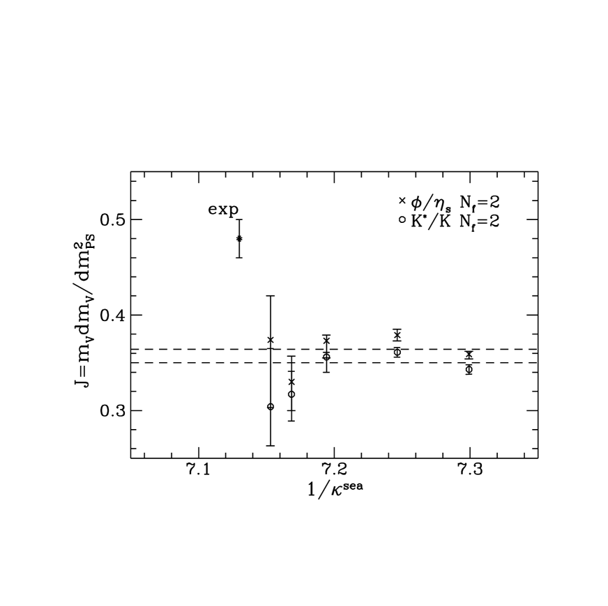
Figure 10: Values of the parameter $J$, determined from fixing the $K^{*}/K$ and $\phi/\eta_{s}$, plotted against $1/\mbox{$\kappa^{\rm sea}$}$ for $V=12^{3}\cdot 24$. The quenched result, taken from [46], is represented by the dashed lines.

The parameter $J$ has been introduced in [44] as a way to quantify the discrepancy between the quenched spectrum and experiment. It is defined as

$$J=m_{K^{*}}\frac{d{m_{\rm V}}}{dm_{\rm PS}^{2}},$$ (46)

and has the attractive feature that it is dimensionless, does not involve extrapolations to the chiral limit and is independent of the quark mass values chosen to evaluate it, provided that $m_{\rm V}$ depends linearly on $m_{\rm PS}^{2}$. The only physical prediction sacrificed to calculate $J$ is the ratio $m_{K^{*}}/m_{K}=1.81$. In the $(m_{\rm PS}^{2},{m_{\rm V}})$ plane this corresponds to a parabola, the intercept of which with the linear interpolation of the simulated data yields the point $(m_{K}^{2},m_{K^{*}})$ of strange mesons. An alternative way to determine $J$ is to use mesons with full strange valence quark content, by assuming that the $\eta_{s}$ is purely $s\overline{s}$ and that $m_{\phi}/m_{\eta_{s}}=1.57$.

We emphasise that a realistic evaluation of $J$ in the dynamical case is not straightforward. As pointed out in [44], it would not be appropriate to compare meson masses obtained using different dynamical quark masses as the lattice spacing $a$ depends on the sea quark mass. Our approach has been to fix the sea quark mass and for each sea quark consider different valence quark masses. Ideally, since we are looking to interpret the valence quarks as having strange flavour in the sea of light quarks, we would need to consider values of $\mbox{$\kappa^{\rm val}$}<\mbox{$\kappa^{\rm sea}$}$. With our present dataset, this is only possible at the most chiral sea quark masses. However, since even our lightest sea quark mass is in the region of that of the strange quark, we do not expect the values of $J$ to be significantly closer to the experimental value of $J=0.48(2)$, compared to the quenched approximation.

In Fig. 10 we show the values of $J$ and compare them with the quenched result at $\beta=5.7$ and $V=12^{3}\cdot 24$ [46]. The values of $J$, obtained by either fixing $m_{K^{*}}/m_{K}$ or $m_{\phi}/m_{\eta_{s}}$ show no appreciable trend towards the experimental point as the sea quark mass decreases. Moreover, the errors are amplified by the fitting process to extract the slope ${d{m_{\rm V}}}/{dm_{\rm PS}^{2}}$, especially at the lightest $\kappa^{\rm sea}$.

Figure 11: Vector mass plotted against the pseudoscalar mass for $V=12^{3}\cdot 24$ for several sets of different sea quark masses. Asterisks denote the experimental points. The quenched results (labelled $\mbox{$\kappa^{\rm sea}$}=0$) are taken from [46].

Another way to look for dynamical quark effects in the light hadron spectrum, which does not involve any fitting, is to concentrate directly on the plot of the vector mass versus the pseudoscalar mass squared. This is shown in Fig. 11. As the sea quark mass is decreased relative to the valence quark mass, one observes a significant, albeit small trend of the meson masses towards the point $(m_{\eta_{s}}^{2},m_{\phi})$, i.e. the pair of mesons, whose valence quark content resembles most closely that used in our simulation. Concentrating on the lighter sea-quark mass, e.g. $\mbox{$\kappa^{\rm sea}$}=0.1395$, we can assert a significant shift compared to the quenched result, at $\beta=5.7$ and $V=12^{3}\cdot 24$ [46].

At this stage it is hard to quantify the observed shift, and to disentangle the genuine sea quark effect from residual lattice artefacts, which could be fairly large in these simulations. A suitable approach would be to monitor dynamical quark effects at fixed lattice spacing. Starting from the quenched approximation, and going to ever lighter sea quark masses, one would have to perform a sequence of simulations, which are matched such that they all reproduce the same value of a suitable lattice scale, e.g. $r_{0}$ [47]. Results will be published in a future publication, using the fully $O(a)$ improved action for dynamical and quenched simulations [18].

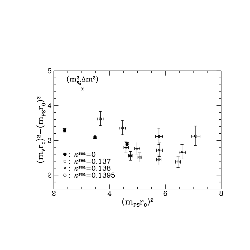
Figure 12: Hyperfine splitting $({m_{\rm V}}r_{0})^{2}-(m_{\rm PS}r_{0})^{2}$ plotted against $(m_{\rm PS}r_{0})^{2}$ for $V=12^{3}\cdot 24$. The quenched results ($\mbox{$\kappa^{\rm sea}$}=0$) are taken from [46].

Another quantity, which can be used to highlight the effects of dynamical quarks, is the vector-pseudoscalar mass splitting. It is well known that lattice simulations fail to reproduce the experimental fact that this hyperfine splitting is constant over a large range of quark masses, $m_{\rm V}^{2}-m_{\rm PS}^{2}\simeq 0.55\,{\rm GeV}^{2}$. The discrepancy between the experimental and (much lower) lattice determinations of $m_{\rm V}^{2}-m_{\rm PS}^{2}$ are partly due to lattice artefacts [48]. However, it is widely expected that the remaining difference, which becomes more pronounced as the valence quark mass is increased, is due to dynamical quark effects. In Fig. 12 we plot the meson hyperfine splitting $({m_{\rm V}}r_{0})^{2}-(m_{\rm PS}r_{0})^{2}$ versus $(m_{\rm PS}r_{0})^{2}$ for all values of $\kappa^{\rm sea}$. The numerical data are compared to the $\phi-\eta_{s}$ splitting. Despite the relatively poor statistical accuracy it is obvious that the numerically determined hyperfine splitting shows a trend towards the experimental point as the sea quark mass is decreased. As regards the quantification of the relative deviation from experiment between the results obtained in the quenched approximation and for finite sea quark mass, the same caveats apply as for the interpretation of Fig. 11, namely, that the comparison should be performed for fixed lattice spacing.

5 Conclusions

In this paper, we have presented the first results on the light hadron spectrum and the static quark potential obtained from dynamical simulations using an $O(a)$ improved fermion action at $\beta=5.2$. Sea quark masses were chosen such that $m_{\rm PS}/m_{\rm V}$ was in the range $0.86$ down to $0.67$. The value of $c_{\rm sw}=1.76$ was not appropriate to remove all leading discretisation effects. We wish to point out, however, that at such a low $\beta$ value residual lattice artefacts could be relatively large, even after full $O(a)$ improvement. This question clearly requires further investigation.

We have addressed the important issue of finite-size effects, which are expected to be larger in dynamical simulations, compared to the quenched approximation. By simulating three different lattice sizes for a range of sea quark masses, we found that finite-size effects are practically absent for box sizes $L\,\,\raisebox{-2.58334pt}{$\stackrel{{\scriptstyle\textstyle{>}}}{{\sim}}$}\,\,1.6\,{\rm fm}$, and sea quark masses which give $m_{\rm PS}/m_{\rm V}\,\,\raisebox{-2.58334pt}{$\stackrel{{\scriptstyle\textstyle{>}}}{{\sim}}$}\,\,0.67$. This is observed in the data for the static quark potential and hadron masses. However, for lighter dynamical quarks one would expect that yet larger volumes are required.

Instead of presenting quantitative results for the light hadron spectrum, we have concentrated on highlighting the effects of dynamical quarks. Although the evidence for string breaking in the data for the static quark potential and for an improved behaviour of the parameter $J$ remains inconclusive, we have detected significant effects due to dynamical quarks. Namely, the Coulombic part of the static quark potential is enhanced for finite sea quark mass, and the vector-pseudoscalar hyperfine splitting moves closer to the experimental value as the sea quark mass is decreased. Furthermore, pairs of $(m_{\rm V}r_{0},(m_{\rm PS}r_{0})^{2})$ show a trend towards experiment when dynamical quarks are “switched on”.

The results presented here serve as a guideline for ongoing investigations, which are performed using the fully $O(a)$ improved action for two flavours of dynamical quarks, whose masses are closer to the chiral limit than those used in this study.

Appendix A Tables

Here we list the meson and baryon masses for all combinations of $\kappa^{\rm sea}$ and $\kappa^{\rm val}$, and on all lattice sizes used in the simulations.

In the following tables we also list the fitting interval and the value of $\chi^{2}/\rm d.o.f.$, obtained from a correlated fit to eqs. (32) or (33), respectively. Some of the fits produce values of $\chi^{2}/\rm d.o.f.$, which would normally be regarded as unacceptably large, even though we are confident that the fit intervals were properly tuned. In such cases we have compared the results for the masses to those obtained using an uncorrelated fit over the same interval. We always found that the uncorrelated fit gave results which, within errors, were perfectly compatible with those from the correlated fit, whilst producing values for $\chi^{2}/\rm d.o.f.$, which were significantly below one. Thus we are confident that the results presented in the tables below are reliable, that a double exponential is an appropriate model function in all cases, but that correlations in the data are clearly present.

$L^{3}\cdot T$	$\kappa^{sea}$	$\kappa^{val}$	${m_{\rm PS}}a$	$m_{\rm PS}r_{0}$	Fit	$\chi^{2}/$ dof
$8^{3}\cdot 24$	0.1370	0.1370	1.119$\;\begin{array}[]{@{}l@{}}\makebox[15.0pt][c]{$+$}\makebox[3.85002pt][r]{ 8}\\[-0.83997pt] \makebox[15.0pt][c]{$-$}\makebox[3.85002pt][r]{ 4}\end{array}$	2.502$\;\begin{array}[]{@{}l@{}}\makebox[15.0pt][c]{$+$}\makebox[3.85002pt][r]{ 47}\\[-0.83997pt] \makebox[15.0pt][c]{$-$}\makebox[3.85002pt][r]{ 52}\end{array}$	[ 6,11]	12.70 / 6
		0.1380	1.059$\;\begin{array}[]{@{}l@{}}\makebox[15.0pt][c]{$+$}\makebox[3.85002pt][r]{ 8}\\[-0.83997pt] \makebox[15.0pt][c]{$-$}\makebox[3.85002pt][r]{ 4}\end{array}$	2.368$\;\begin{array}[]{@{}l@{}}\makebox[15.0pt][c]{$+$}\makebox[3.85002pt][r]{ 45}\\[-0.83997pt] \makebox[15.0pt][c]{$-$}\makebox[3.85002pt][r]{ 50}\end{array}$	[ 6,11]	12.77 / 6
		0.1390	0.997$\;\begin{array}[]{@{}l@{}}\makebox[15.0pt][c]{$+$}\makebox[3.85002pt][r]{ 9}\\[-0.83997pt] \makebox[15.0pt][c]{$-$}\makebox[3.85002pt][r]{ 5}\end{array}$	2.229$\;\begin{array}[]{@{}l@{}}\makebox[15.0pt][c]{$+$}\makebox[3.85002pt][r]{ 44}\\[-0.83997pt] \makebox[15.0pt][c]{$-$}\makebox[3.85002pt][r]{ 47}\end{array}$	[ 6,11]	13.20 / 6
		0.1395	0.965$\;\begin{array}[]{@{}l@{}}\makebox[15.0pt][c]{$+$}\makebox[3.85002pt][r]{ 9}\\[-0.83997pt] \makebox[15.0pt][c]{$-$}\makebox[3.85002pt][r]{ 4}\end{array}$	2.158$\;\begin{array}[]{@{}l@{}}\makebox[15.0pt][c]{$+$}\makebox[3.85002pt][r]{ 43}\\[-0.83997pt] \makebox[15.0pt][c]{$-$}\makebox[3.85002pt][r]{ 45}\end{array}$	[ 6,11]	13.57 / 6
$8^{3}\cdot 24$	0.1380	0.1370	1.011$\;\begin{array}[]{@{}l@{}}\makebox[15.0pt][c]{$+$}\makebox[3.85002pt][r]{ 10}\\[-0.83997pt] \makebox[15.0pt][c]{$-$}\makebox[3.85002pt][r]{ 2}\end{array}$	2.502$\;\begin{array}[]{@{}l@{}}\makebox[15.0pt][c]{$+$}\makebox[3.85002pt][r]{ 79}\\[-0.83997pt] \makebox[15.0pt][c]{$-$}\makebox[3.85002pt][r]{ 68}\end{array}$	[ 5,11]	14.94 / 8
		0.1380	0.945$\;\begin{array}[]{@{}l@{}}\makebox[15.0pt][c]{$+$}\makebox[3.85002pt][r]{ 11}\\[-0.83997pt] \makebox[15.0pt][c]{$-$}\makebox[3.85002pt][r]{ 2}\end{array}$	2.339$\;\begin{array}[]{@{}l@{}}\makebox[15.0pt][c]{$+$}\makebox[3.85002pt][r]{ 75}\\[-0.83997pt] \makebox[15.0pt][c]{$-$}\makebox[3.85002pt][r]{ 64}\end{array}$	[ 5,11]	13.28 / 8
		0.1390	0.874$\;\begin{array}[]{@{}l@{}}\makebox[15.0pt][c]{$+$}\makebox[3.85002pt][r]{ 12}\\[-0.83997pt] \makebox[15.0pt][c]{$-$}\makebox[3.85002pt][r]{ 6}\end{array}$	2.164$\;\begin{array}[]{@{}l@{}}\makebox[15.0pt][c]{$+$}\makebox[3.85002pt][r]{ 72}\\[-0.83997pt] \makebox[15.0pt][c]{$-$}\makebox[3.85002pt][r]{ 61}\end{array}$	[ 5,11]	7.26 / 8
		0.1395	0.840$\;\begin{array}[]{@{}l@{}}\makebox[15.0pt][c]{$+$}\makebox[3.85002pt][r]{ 14}\\[-0.83997pt] \makebox[15.0pt][c]{$-$}\makebox[3.85002pt][r]{ 6}\end{array}$	2.078$\;\begin{array}[]{@{}l@{}}\makebox[15.0pt][c]{$+$}\makebox[3.85002pt][r]{ 71}\\[-0.83997pt] \makebox[15.0pt][c]{$-$}\makebox[3.85002pt][r]{ 58}\end{array}$	[ 5,11]	7.50 / 8
$8^{3}\cdot 24$	0.1390	0.1370	0.870$\;\begin{array}[]{@{}l@{}}\makebox[15.0pt][c]{$+$}\makebox[3.85002pt][r]{ 9}\\[-0.83997pt] \makebox[15.0pt][c]{$-$}\makebox[3.85002pt][r]{ 5}\end{array}$	2.514$\;\begin{array}[]{@{}l@{}}\makebox[15.0pt][c]{$+$}\makebox[3.85002pt][r]{ 58}\\[-0.83997pt] \makebox[15.0pt][c]{$-$}\makebox[3.85002pt][r]{ 53}\end{array}$	[ 6,11]	8.14 / 6
		0.1380	0.799$\;\begin{array}[]{@{}l@{}}\makebox[15.0pt][c]{$+$}\makebox[3.85002pt][r]{ 10}\\[-0.83997pt] \makebox[15.0pt][c]{$-$}\makebox[3.85002pt][r]{ 5}\end{array}$	2.309$\;\begin{array}[]{@{}l@{}}\makebox[15.0pt][c]{$+$}\makebox[3.85002pt][r]{ 57}\\[-0.83997pt] \makebox[15.0pt][c]{$-$}\makebox[3.85002pt][r]{ 49}\end{array}$	[ 6,11]	8.18 / 6
		0.1390	0.726$\;\begin{array}[]{@{}l@{}}\makebox[15.0pt][c]{$+$}\makebox[3.85002pt][r]{ 11}\\[-0.83997pt] \makebox[15.0pt][c]{$-$}\makebox[3.85002pt][r]{ 6}\end{array}$	2.099$\;\begin{array}[]{@{}l@{}}\makebox[15.0pt][c]{$+$}\makebox[3.85002pt][r]{ 53}\\[-0.83997pt] \makebox[15.0pt][c]{$-$}\makebox[3.85002pt][r]{ 45}\end{array}$	[ 5,11]	10.24 / 8
		0.1395	0.686$\;\begin{array}[]{@{}l@{}}\makebox[15.0pt][c]{$+$}\makebox[3.85002pt][r]{ 12}\\[-0.83997pt] \makebox[15.0pt][c]{$-$}\makebox[3.85002pt][r]{ 5}\end{array}$	1.982$\;\begin{array}[]{@{}l@{}}\makebox[15.0pt][c]{$+$}\makebox[3.85002pt][r]{ 53}\\[-0.83997pt] \makebox[15.0pt][c]{$-$}\makebox[3.85002pt][r]{ 43}\end{array}$	[ 5,11]	10.86 / 8
$8^{3}\cdot 24$	0.1395	0.1370	0.786$\;\begin{array}[]{@{}l@{}}\makebox[15.0pt][c]{$+$}\makebox[3.85002pt][r]{ 9}\\[-0.83997pt] \makebox[15.0pt][c]{$-$}\makebox[3.85002pt][r]{ 14}\end{array}$	2.924$\;\begin{array}[]{@{}l@{}}\makebox[15.0pt][c]{$+$}\makebox[3.85002pt][r]{ 78}\\[-0.83997pt] \makebox[15.0pt][c]{$-$}\makebox[3.85002pt][r]{ 78}\end{array}$	[ 6,11]	9.70 / 6
		0.1380	0.710$\;\begin{array}[]{@{}l@{}}\makebox[15.0pt][c]{$+$}\makebox[3.85002pt][r]{ 9}\\[-0.83997pt] \makebox[15.0pt][c]{$-$}\makebox[3.85002pt][r]{ 12}\end{array}$	2.640$\;\begin{array}[]{@{}l@{}}\makebox[15.0pt][c]{$+$}\makebox[3.85002pt][r]{ 72}\\[-0.83997pt] \makebox[15.0pt][c]{$-$}\makebox[3.85002pt][r]{ 68}\end{array}$	[ 6,11]	10.75 / 6
		0.1390	0.642$\;\begin{array}[]{@{}l@{}}\makebox[15.0pt][c]{$+$}\makebox[3.85002pt][r]{ 15}\\[-0.83997pt] \makebox[15.0pt][c]{$-$}\makebox[3.85002pt][r]{ 10}\end{array}$	2.387$\;\begin{array}[]{@{}l@{}}\makebox[15.0pt][c]{$+$}\makebox[3.85002pt][r]{ 80}\\[-0.83997pt] \makebox[15.0pt][c]{$-$}\makebox[3.85002pt][r]{ 60}\end{array}$	[ 5,11]	15.07 / 8
		0.1395	0.603$\;\begin{array}[]{@{}l@{}}\makebox[15.0pt][c]{$+$}\makebox[3.85002pt][r]{ 17}\\[-0.83997pt] \makebox[15.0pt][c]{$-$}\makebox[3.85002pt][r]{ 7}\end{array}$	2.242$\;\begin{array}[]{@{}l@{}}\makebox[15.0pt][c]{$+$}\makebox[3.85002pt][r]{ 82}\\[-0.83997pt] \makebox[15.0pt][c]{$-$}\makebox[3.85002pt][r]{ 51}\end{array}$	[ 4,11]	17.30 / 10

Table 6: Pseudoscalar masses on $8^{3}\cdot 24$, in lattice units and in units of $r_{0}$.

$L^{3}\cdot T$	$\kappa^{sea}$	$\kappa^{val}$	${m_{\rm PS}}a$	$m_{\rm PS}r_{0}$	Fit	$\chi^{2}/$ dof
$12^{3}\cdot 24$	0.1370	0.1370	1.108$\;\begin{array}[]{@{}l@{}}\makebox[15.0pt][c]{$+$}\makebox[3.85002pt][r]{ 3}\\[-0.83997pt] \makebox[15.0pt][c]{$-$}\makebox[3.85002pt][r]{ 2}\end{array}$	2.541$\;\begin{array}[]{@{}l@{}}\makebox[15.0pt][c]{$+$}\makebox[3.85002pt][r]{ 23}\\[-0.83997pt] \makebox[15.0pt][c]{$-$}\makebox[3.85002pt][r]{ 26}\end{array}$	[ 6,11]	9.93 / 6
		0.1380	1.047$\;\begin{array}[]{@{}l@{}}\makebox[15.0pt][c]{$+$}\makebox[3.85002pt][r]{ 3}\\[-0.83997pt] \makebox[15.0pt][c]{$-$}\makebox[3.85002pt][r]{ 2}\end{array}$	2.402$\;\begin{array}[]{@{}l@{}}\makebox[15.0pt][c]{$+$}\makebox[3.85002pt][r]{ 22}\\[-0.83997pt] \makebox[15.0pt][c]{$-$}\makebox[3.85002pt][r]{ 25}\end{array}$	[ 5,11]	11.18 / 8
		0.1390	0.983$\;\begin{array}[]{@{}l@{}}\makebox[15.0pt][c]{$+$}\makebox[3.85002pt][r]{ 4}\\[-0.83997pt] \makebox[15.0pt][c]{$-$}\makebox[3.85002pt][r]{ 2}\end{array}$	2.255$\;\begin{array}[]{@{}l@{}}\makebox[15.0pt][c]{$+$}\makebox[3.85002pt][r]{ 21}\\[-0.83997pt] \makebox[15.0pt][c]{$-$}\makebox[3.85002pt][r]{ 23}\end{array}$	[ 5,11]	11.65 / 8
		0.1395	0.950$\;\begin{array}[]{@{}l@{}}\makebox[15.0pt][c]{$+$}\makebox[3.85002pt][r]{ 4}\\[-0.83997pt] \makebox[15.0pt][c]{$-$}\makebox[3.85002pt][r]{ 3}\end{array}$	2.179$\;\begin{array}[]{@{}l@{}}\makebox[15.0pt][c]{$+$}\makebox[3.85002pt][r]{ 21}\\[-0.83997pt] \makebox[15.0pt][c]{$-$}\makebox[3.85002pt][r]{ 23}\end{array}$	[ 5,11]	11.83 / 8
$12^{3}\cdot 24$	0.1380	0.1370	1.000$\;\begin{array}[]{@{}l@{}}\makebox[15.0pt][c]{$+$}\makebox[3.85002pt][r]{ 3}\\[-0.83997pt] \makebox[15.0pt][c]{$-$}\makebox[3.85002pt][r]{ 2}\end{array}$	2.569$\;\begin{array}[]{@{}l@{}}\makebox[15.0pt][c]{$+$}\makebox[3.85002pt][r]{ 35}\\[-0.83997pt] \makebox[15.0pt][c]{$-$}\makebox[3.85002pt][r]{ 30}\end{array}$	[ 6,11]	10.41 / 6
		0.1380	0.936$\;\begin{array}[]{@{}l@{}}\makebox[15.0pt][c]{$+$}\makebox[3.85002pt][r]{ 3}\\[-0.83997pt] \makebox[15.0pt][c]{$-$}\makebox[3.85002pt][r]{ 2}\end{array}$	2.404$\;\begin{array}[]{@{}l@{}}\makebox[15.0pt][c]{$+$}\makebox[3.85002pt][r]{ 33}\\[-0.83997pt] \makebox[15.0pt][c]{$-$}\makebox[3.85002pt][r]{ 29}\end{array}$	[ 6,11]	10.79 / 6
		0.1390	0.869$\;\begin{array}[]{@{}l@{}}\makebox[15.0pt][c]{$+$}\makebox[3.85002pt][r]{ 4}\\[-0.83997pt] \makebox[15.0pt][c]{$-$}\makebox[3.85002pt][r]{ 2}\end{array}$	2.232$\;\begin{array}[]{@{}l@{}}\makebox[15.0pt][c]{$+$}\makebox[3.85002pt][r]{ 31}\\[-0.83997pt] \makebox[15.0pt][c]{$-$}\makebox[3.85002pt][r]{ 27}\end{array}$	[ 6,11]	11.37 / 6
		0.1395	0.834$\;\begin{array}[]{@{}l@{}}\makebox[15.0pt][c]{$+$}\makebox[3.85002pt][r]{ 4}\\[-0.83997pt] \makebox[15.0pt][c]{$-$}\makebox[3.85002pt][r]{ 2}\end{array}$	2.142$\;\begin{array}[]{@{}l@{}}\makebox[15.0pt][c]{$+$}\makebox[3.85002pt][r]{ 30}\\[-0.83997pt] \makebox[15.0pt][c]{$-$}\makebox[3.85002pt][r]{ 26}\end{array}$	[ 6,11]	11.56 / 6
$12^{3}\cdot 24$	0.1390	0.1370	0.858$\;\begin{array}[]{@{}l@{}}\makebox[15.0pt][c]{$+$}\makebox[3.85002pt][r]{ 4}\\[-0.83997pt] \makebox[15.0pt][c]{$-$}\makebox[3.85002pt][r]{ 3}\end{array}$	2.613$\;\begin{array}[]{@{}l@{}}\makebox[15.0pt][c]{$+$}\makebox[3.85002pt][r]{ 51}\\[-0.83997pt] \makebox[15.0pt][c]{$-$}\makebox[3.85002pt][r]{ 45}\end{array}$	[ 7,11]	5.93 / 4
		0.1380	0.785$\;\begin{array}[]{@{}l@{}}\makebox[15.0pt][c]{$+$}\makebox[3.85002pt][r]{ 4}\\[-0.83997pt] \makebox[15.0pt][c]{$-$}\makebox[3.85002pt][r]{ 3}\end{array}$	2.391$\;\begin{array}[]{@{}l@{}}\makebox[15.0pt][c]{$+$}\makebox[3.85002pt][r]{ 48}\\[-0.83997pt] \makebox[15.0pt][c]{$-$}\makebox[3.85002pt][r]{ 42}\end{array}$	[ 7,11]	4.16 / 4
		0.1390	0.707$\;\begin{array}[]{@{}l@{}}\makebox[15.0pt][c]{$+$}\makebox[3.85002pt][r]{ 5}\\[-0.83997pt] \makebox[15.0pt][c]{$-$}\makebox[3.85002pt][r]{ 3}\end{array}$	2.155$\;\begin{array}[]{@{}l@{}}\makebox[15.0pt][c]{$+$}\makebox[3.85002pt][r]{ 44}\\[-0.83997pt] \makebox[15.0pt][c]{$-$}\makebox[3.85002pt][r]{ 38}\end{array}$	[ 7,11]	2.69 / 4
		0.1395	0.669$\;\begin{array}[]{@{}l@{}}\makebox[15.0pt][c]{$+$}\makebox[3.85002pt][r]{ 5}\\[-0.83997pt] \makebox[15.0pt][c]{$-$}\makebox[3.85002pt][r]{ 3}\end{array}$	2.037$\;\begin{array}[]{@{}l@{}}\makebox[15.0pt][c]{$+$}\makebox[3.85002pt][r]{ 42}\\[-0.83997pt] \makebox[15.0pt][c]{$-$}\makebox[3.85002pt][r]{ 36}\end{array}$	[ 6,11]	16.86 / 6
$12^{3}\cdot 24$	0.1395	0.1370	0.775$\;\begin{array}[]{@{}l@{}}\makebox[15.0pt][c]{$+$}\makebox[3.85002pt][r]{ 6}\\[-0.83997pt] \makebox[15.0pt][c]{$-$}\makebox[3.85002pt][r]{ 4}\end{array}$	2.662$\;\begin{array}[]{@{}l@{}}\makebox[15.0pt][c]{$+$}\makebox[3.85002pt][r]{ 42}\\[-0.83997pt] \makebox[15.0pt][c]{$-$}\makebox[3.85002pt][r]{ 39}\end{array}$	[ 7,11]	21.46 / 4
		0.1380	0.699$\;\begin{array}[]{@{}l@{}}\makebox[15.0pt][c]{$+$}\makebox[3.85002pt][r]{ 5}\\[-0.83997pt] \makebox[15.0pt][c]{$-$}\makebox[3.85002pt][r]{ 4}\end{array}$	2.402$\;\begin{array}[]{@{}l@{}}\makebox[15.0pt][c]{$+$}\makebox[3.85002pt][r]{ 38}\\[-0.83997pt] \makebox[15.0pt][c]{$-$}\makebox[3.85002pt][r]{ 36}\end{array}$	[ 6,11]	26.14 / 6
		0.1390	0.615$\;\begin{array}[]{@{}l@{}}\makebox[15.0pt][c]{$+$}\makebox[3.85002pt][r]{ 6}\\[-0.83997pt] \makebox[15.0pt][c]{$-$}\makebox[3.85002pt][r]{ 4}\end{array}$	2.112$\;\begin{array}[]{@{}l@{}}\makebox[15.0pt][c]{$+$}\makebox[3.85002pt][r]{ 36}\\[-0.83997pt] \makebox[15.0pt][c]{$-$}\makebox[3.85002pt][r]{ 32}\end{array}$	[ 6,11]	19.70 / 6
		0.1395	0.558$\;\begin{array}[]{@{}l@{}}\makebox[15.0pt][c]{$+$}\makebox[3.85002pt][r]{ 8}\\[-0.83997pt] \makebox[15.0pt][c]{$-$}\makebox[3.85002pt][r]{ 7}\end{array}$	1.916$\;\begin{array}[]{@{}l@{}}\makebox[15.0pt][c]{$+$}\makebox[3.85002pt][r]{ 38}\\[-0.83997pt] \makebox[15.0pt][c]{$-$}\makebox[3.85002pt][r]{ 35}\end{array}$	[ 5,11]	8.96 / 8
$12^{3}\cdot 24$	0.1398	0.1380	0.639$\;\begin{array}[]{@{}l@{}}\makebox[15.0pt][c]{$+$}\makebox[3.85002pt][r]{ 5}\\[-0.83997pt] \makebox[15.0pt][c]{$-$}\makebox[3.85002pt][r]{ 4}\end{array}$	2.332$\;\begin{array}[]{@{}l@{}}\makebox[15.0pt][c]{$+$}\makebox[3.85002pt][r]{ 27}\\[-0.83997pt] \makebox[15.0pt][c]{$-$}\makebox[3.85002pt][r]{ 21}\end{array}$	[ 7,11]	3.63 / 4
		0.1390	0.551$\;\begin{array}[]{@{}l@{}}\makebox[15.0pt][c]{$+$}\makebox[3.85002pt][r]{ 4}\\[-0.83997pt] \makebox[15.0pt][c]{$-$}\makebox[3.85002pt][r]{ 9}\end{array}$	2.011$\;\begin{array}[]{@{}l@{}}\makebox[15.0pt][c]{$+$}\makebox[3.85002pt][r]{ 23}\\[-0.83997pt] \makebox[15.0pt][c]{$-$}\makebox[3.85002pt][r]{ 37}\end{array}$	[ 7,11]	2.09 / 4
		0.1395	0.492$\;\begin{array}[]{@{}l@{}}\makebox[15.0pt][c]{$+$}\makebox[3.85002pt][r]{ 3}\\[-0.83997pt] \makebox[15.0pt][c]{$-$}\makebox[3.85002pt][r]{ 9}\end{array}$	1.797$\;\begin{array}[]{@{}l@{}}\makebox[15.0pt][c]{$+$}\makebox[3.85002pt][r]{ 18}\\[-0.83997pt] \makebox[15.0pt][c]{$-$}\makebox[3.85002pt][r]{ 36}\end{array}$	[ 6,11]	3.41 / 6
		0.1398	0.476$\;\begin{array}[]{@{}l@{}}\makebox[15.0pt][c]{$+$}\makebox[3.85002pt][r]{ 3}\\[-0.83997pt] \makebox[15.0pt][c]{$-$}\makebox[3.85002pt][r]{ 16}\end{array}$	1.738$\;\begin{array}[]{@{}l@{}}\makebox[15.0pt][c]{$+$}\makebox[3.85002pt][r]{ 17}\\[-0.83997pt] \makebox[15.0pt][c]{$-$}\makebox[3.85002pt][r]{ 61}\end{array}$	[ 6,11]	8.14 / 6

Table 7: Pseudoscalar masses on $12^{3}\cdot 24$, in lattice units and in units of $r_{0}$.

$L^{3}\cdot T$	$\kappa^{sea}$	$\kappa^{val}$	${m_{\rm PS}}a$	$m_{\rm PS}r_{0}$	Fit	$\chi^{2}/$ dof
$16^{3}\cdot 24$	0.1390	0.1390	0.701$\;\begin{array}[]{@{}l@{}}\makebox[15.0pt][c]{$+$}\makebox[1.04996pt][r]{ 6}\\[-0.83997pt] \makebox[15.0pt][c]{$-$}\makebox[1.04996pt][r]{ 5}\end{array}$	2.120$\;\begin{array}[]{@{}l@{}}\makebox[15.0pt][c]{$+$}\makebox[3.85002pt][r]{ 30}\\[-0.83997pt] \makebox[15.0pt][c]{$-$}\makebox[3.85002pt][r]{ 22}\end{array}$	[ 6,11]	10.62 / 6
		0.1395	0.660$\;\begin{array}[]{@{}l@{}}\makebox[15.0pt][c]{$+$}\makebox[1.04996pt][r]{ 6}\\[-0.83997pt] \makebox[15.0pt][c]{$-$}\makebox[1.04996pt][r]{ 4}\end{array}$	1.998$\;\begin{array}[]{@{}l@{}}\makebox[15.0pt][c]{$+$}\makebox[3.85002pt][r]{ 28}\\[-0.83997pt] \makebox[15.0pt][c]{$-$}\makebox[3.85002pt][r]{ 21}\end{array}$	[ 6,11]	9.31 / 6
		0.1398	0.635$\;\begin{array}[]{@{}l@{}}\makebox[15.0pt][c]{$+$}\makebox[1.04996pt][r]{ 6}\\[-0.83997pt] \makebox[15.0pt][c]{$-$}\makebox[1.04996pt][r]{ 5}\end{array}$	1.922$\;\begin{array}[]{@{}l@{}}\makebox[15.0pt][c]{$+$}\makebox[3.85002pt][r]{27}\\[-0.83997pt] \makebox[15.0pt][c]{$-$}\makebox[3.85002pt][r]{ 22}\end{array}$	[ 6,11]	8.34 / 6
$16^{3}\cdot 24$	0.1395	0.1390	0.610$\;\begin{array}[]{@{}l@{}}\makebox[15.0pt][c]{$+$}\makebox[1.04996pt][r]{ 4}\\[-0.83997pt] \makebox[15.0pt][c]{$-$}\makebox[1.04996pt][r]{ 2}\end{array}$	2.101$\;\begin{array}[]{@{}l@{}}\makebox[15.0pt][c]{$+$}\makebox[3.85002pt][r]{ 28}\\[-0.83997pt] \makebox[15.0pt][c]{$-$}\makebox[3.85002pt][r]{ 36}\end{array}$	[ 6,11]	7.04 / 6
		0.1395	0.564$\;\begin{array}[]{@{}l@{}}\makebox[15.0pt][c]{$+$}\makebox[1.04996pt][r]{ 3}\\[-0.83997pt] \makebox[15.0pt][c]{$-$}\makebox[1.04996pt][r]{ 4}\end{array}$	1.942$\;\begin{array}[]{@{}l@{}}\makebox[15.0pt][c]{$+$}\makebox[3.85002pt][r]{ 25}\\[-0.83997pt] \makebox[15.0pt][c]{$-$}\makebox[3.85002pt][r]{ 36}\end{array}$	[ 6,11]	3.05 / 6
		0.1398	0.537$\;\begin{array}[]{@{}l@{}}\makebox[15.0pt][c]{$+$}\makebox[1.04996pt][r]{ 4}\\[-0.83997pt] \makebox[15.0pt][c]{$-$}\makebox[1.04996pt][r]{ 3}\end{array}$	1.848$\;\begin{array}[]{@{}l@{}}\makebox[15.0pt][c]{$+$}\makebox[3.85002pt][r]{ 26}\\[-0.83997pt] \makebox[15.0pt][c]{$-$}\makebox[3.85002pt][r]{ 32}\end{array}$	[ 7,11]	2.99 / 4
$16^{3}\cdot 24$	0.1398	0.1390	0.551$\;\begin{array}[]{@{}l@{}}\makebox[15.0pt][c]{$+$}\makebox[1.04996pt][r]{ 5}\\[-0.83997pt] \makebox[15.0pt][c]{$-$}\makebox[1.04996pt][r]{ 5}\end{array}$	2.011$\;\begin{array}[]{@{}l@{}}\makebox[15.0pt][c]{$+$}\makebox[3.85002pt][r]{ 26}\\[-0.83997pt] \makebox[15.0pt][c]{$-$}\makebox[3.85002pt][r]{ 26}\end{array}$	[ 7,11]	10.66 / 4
		0.1395	0.502$\;\begin{array}[]{@{}l@{}}\makebox[15.0pt][c]{$+$}\makebox[1.04996pt][r]{ 5}\\[-0.83997pt] \makebox[15.0pt][c]{$-$}\makebox[1.04996pt][r]{ 6}\end{array}$	1.834$\;\begin{array}[]{@{}l@{}}\makebox[15.0pt][c]{$+$}\makebox[3.85002pt][r]{ 24}\\[-0.83997pt] \makebox[15.0pt][c]{$-$}\makebox[3.85002pt][r]{ 28}\end{array}$	[ 7,11]	8.48 / 4
		0.1398	0.468$\;\begin{array}[]{@{}l@{}}\makebox[15.0pt][c]{$+$}\makebox[1.04996pt][r]{ 5}\\[-0.83997pt] \makebox[15.0pt][c]{$-$}\makebox[1.04996pt][r]{ 5}\end{array}$	1.707$\;\begin{array}[]{@{}l@{}}\makebox[15.0pt][c]{$+$}\makebox[3.85002pt][r]{ 23}\\[-0.83997pt] \makebox[15.0pt][c]{$-$}\makebox[3.85002pt][r]{ 24}\end{array}$	[ 7,11]	6.02 / 4

Table 8: Pseudoscalar masses on $16^{3}\cdot 24$, in lattice units and in units of $r_{0}$.

$L^{3}\cdot T$	$\kappa^{sea}$	$\kappa^{val}$	${m_{\rm V}}a$	${m_{\rm V}}r_{0}$	Fit	$\chi^{2}/$ dof
$8^{3}\cdot 24$	0.1370	0.1370	1.305$\;\begin{array}[]{@{}l@{}}\makebox[15.0pt][c]{$+$}\makebox[3.85002pt][r]{ 11}\\[-0.83997pt] \makebox[15.0pt][c]{$-$}\makebox[3.85002pt][r]{ 6}\end{array}$	2.917$\;\begin{array}[]{@{}l@{}}\makebox[15.0pt][c]{$+$}\makebox[6.29996pt][r]{ 57}\\[-0.83997pt] \makebox[15.0pt][c]{$-$}\makebox[6.29996pt][r]{ 61}\end{array}$	[ 7,11]	5.82 / 4
		0.1380	1.257$\;\begin{array}[]{@{}l@{}}\makebox[15.0pt][c]{$+$}\makebox[3.85002pt][r]{ 12}\\[-0.83997pt] \makebox[15.0pt][c]{$-$}\makebox[3.85002pt][r]{ 6}\end{array}$	2.810$\;\begin{array}[]{@{}l@{}}\makebox[15.0pt][c]{$+$}\makebox[6.29996pt][r]{ 56}\\[-0.83997pt] \makebox[15.0pt][c]{$-$}\makebox[6.29996pt][r]{ 59}\end{array}$	[ 7,11]	5.09 / 4
		0.1390	1.209$\;\begin{array}[]{@{}l@{}}\makebox[15.0pt][c]{$+$}\makebox[3.85002pt][r]{ 14}\\[-0.83997pt] \makebox[15.0pt][c]{$-$}\makebox[3.85002pt][r]{ 7}\end{array}$	2.703$\;\begin{array}[]{@{}l@{}}\makebox[15.0pt][c]{$+$}\makebox[6.29996pt][r]{ 56}\\[-0.83997pt] \makebox[15.0pt][c]{$-$}\makebox[6.29996pt][r]{ 58}\end{array}$	[ 7,11]	5.27 / 4
		0.1395	1.185$\;\begin{array}[]{@{}l@{}}\makebox[15.0pt][c]{$+$}\makebox[3.85002pt][r]{ 14}\\[-0.83997pt] \makebox[15.0pt][c]{$-$}\makebox[3.85002pt][r]{ 8}\end{array}$	2.650$\;\begin{array}[]{@{}l@{}}\makebox[15.0pt][c]{$+$}\makebox[6.29996pt][r]{ 56}\\[-0.83997pt] \makebox[15.0pt][c]{$-$}\makebox[6.29996pt][r]{ 57}\end{array}$	[ 7,11]	5.78 / 4
$8^{3}\cdot 24$	0.1380	0.1370	1.190$\;\begin{array}[]{@{}l@{}}\makebox[15.0pt][c]{$+$}\makebox[3.85002pt][r]{ 14}\\[-0.83997pt] \makebox[15.0pt][c]{$-$}\makebox[3.85002pt][r]{ 7}\end{array}$	2.946$\;\begin{array}[]{@{}l@{}}\makebox[15.0pt][c]{$+$}\makebox[6.29996pt][r]{ 95}\\[-0.83997pt] \makebox[15.0pt][c]{$-$}\makebox[6.29996pt][r]{ 82}\end{array}$	[ 6,11]	7.30 / 6
		0.1380	1.140$\;\begin{array}[]{@{}l@{}}\makebox[15.0pt][c]{$+$}\makebox[3.85002pt][r]{ 15}\\[-0.83997pt] \makebox[15.0pt][c]{$-$}\makebox[3.85002pt][r]{ 8}\end{array}$	2.822$\;\begin{array}[]{@{}l@{}}\makebox[15.0pt][c]{$+$}\makebox[6.29996pt][r]{ 92}\\[-0.83997pt] \makebox[15.0pt][c]{$-$}\makebox[6.29996pt][r]{ 79}\end{array}$	[ 6,11]	7.68 / 6
		0.1390	1.090$\;\begin{array}[]{@{}l@{}}\makebox[15.0pt][c]{$+$}\makebox[3.85002pt][r]{ 16}\\[-0.83997pt] \makebox[15.0pt][c]{$-$}\makebox[3.85002pt][r]{ 9}\end{array}$	2.697$\;\begin{array}[]{@{}l@{}}\makebox[15.0pt][c]{$+$}\makebox[6.29996pt][r]{ 90}\\[-0.83997pt] \makebox[15.0pt][c]{$-$}\makebox[6.29996pt][r]{ 76}\end{array}$	[ 6,11]	9.02 / 6
		0.1395	1.064$\;\begin{array}[]{@{}l@{}}\makebox[15.0pt][c]{$+$}\makebox[3.85002pt][r]{ 17}\\[-0.83997pt] \makebox[15.0pt][c]{$-$}\makebox[3.85002pt][r]{ 10}\end{array}$	2.634$\;\begin{array}[]{@{}l@{}}\makebox[15.0pt][c]{$+$}\makebox[6.29996pt][r]{ 89}\\[-0.83997pt] \makebox[15.0pt][c]{$-$}\makebox[6.29996pt][r]{ 76}\end{array}$	[ 6,11]	10.05 / 6
$8^{3}\cdot 24$	0.1390	0.1370	1.045$\;\begin{array}[]{@{}l@{}}\makebox[15.0pt][c]{$+$}\makebox[3.85002pt][r]{ 13}\\[-0.83997pt] \makebox[15.0pt][c]{$-$}\makebox[3.85002pt][r]{ 7}\end{array}$	3.022$\;\begin{array}[]{@{}l@{}}\makebox[15.0pt][c]{$+$}\makebox[6.29996pt][r]{ 72}\\[-0.83997pt] \makebox[15.0pt][c]{$-$}\makebox[6.29996pt][r]{ 64}\end{array}$	[ 7,11]	5.21 / 4
		0.1380	0.998$\;\begin{array}[]{@{}l@{}}\makebox[15.0pt][c]{$+$}\makebox[3.85002pt][r]{ 16}\\[-0.83997pt] \makebox[15.0pt][c]{$-$}\makebox[3.85002pt][r]{ 9}\end{array}$	2.885$\;\begin{array}[]{@{}l@{}}\makebox[15.0pt][c]{$+$}\makebox[6.29996pt][r]{ 76}\\[-0.83997pt] \makebox[15.0pt][c]{$-$}\makebox[6.29996pt][r]{ 64}\end{array}$	[ 6,11]	6.49 / 6
		0.1390	0.944$\;\begin{array}[]{@{}l@{}}\makebox[15.0pt][c]{$+$}\makebox[3.85002pt][r]{ 19}\\[-0.83997pt] \makebox[15.0pt][c]{$-$}\makebox[3.85002pt][r]{ 10}\end{array}$	2.730$\;\begin{array}[]{@{}l@{}}\makebox[15.0pt][c]{$+$}\makebox[6.29996pt][r]{ 79}\\[-0.83997pt] \makebox[15.0pt][c]{$-$}\makebox[6.29996pt][r]{ 61}\end{array}$	[ 6,11]	4.66 / 6
		0.1395	0.918$\;\begin{array}[]{@{}l@{}}\makebox[15.0pt][c]{$+$}\makebox[3.85002pt][r]{ 20}\\[-0.83997pt] \makebox[15.0pt][c]{$-$}\makebox[3.85002pt][r]{ 10}\end{array}$	2.653$\;\begin{array}[]{@{}l@{}}\makebox[15.0pt][c]{$+$}\makebox[6.29996pt][r]{ 80}\\[-0.83997pt] \makebox[15.0pt][c]{$-$}\makebox[6.29996pt][r]{ 61}\end{array}$	[ 6,11]	4.08 / 6
$8^{3}\cdot 24$	0.1395	0.1370	0.961$\;\begin{array}[]{@{}l@{}}\makebox[15.0pt][c]{$+$}\makebox[3.85002pt][r]{ 30}\\[-0.83997pt] \makebox[15.0pt][c]{$-$}\makebox[3.85002pt][r]{ 9}\end{array}$	3.573$\;\begin{array}[]{@{}l@{}}\makebox[15.0pt][c]{$+$}\makebox[6.29996pt][r]{141}\\[-0.83997pt] \makebox[15.0pt][c]{$-$}\makebox[6.29996pt][r]{ 77}\end{array}$	[ 7,11]	12.79 / 4
		0.1380	0.917$\;\begin{array}[]{@{}l@{}}\makebox[15.0pt][c]{$+$}\makebox[3.85002pt][r]{ 24}\\[-0.83997pt] \makebox[15.0pt][c]{$-$}\makebox[3.85002pt][r]{ 6}\end{array}$	3.411$\;\begin{array}[]{@{}l@{}}\makebox[15.0pt][c]{$+$}\makebox[6.29996pt][r]{122}\\[-0.83997pt] \makebox[15.0pt][c]{$-$}\makebox[6.29996pt][r]{ 70}\end{array}$	[ 6,11]	11.80 / 6
		0.1390	0.874$\;\begin{array}[]{@{}l@{}}\makebox[15.0pt][c]{$+$}\makebox[3.85002pt][r]{ 34}\\[-0.83997pt] \makebox[15.0pt][c]{$-$}\makebox[3.85002pt][r]{ 5}\end{array}$	3.251$\;\begin{array}[]{@{}l@{}}\makebox[15.0pt][c]{$+$}\makebox[6.29996pt][r]{149}\\[-0.83997pt] \makebox[15.0pt][c]{$-$}\makebox[6.29996pt][r]{ 65}\end{array}$	[ 6,11]	11.01 / 6
		0.1395	0.850$\;\begin{array}[]{@{}l@{}}\makebox[15.0pt][c]{$+$}\makebox[3.85002pt][r]{ 26}\\[-0.83997pt] \makebox[15.0pt][c]{$-$}\makebox[3.85002pt][r]{ 9}\end{array}$	3.159$\;\begin{array}[]{@{}l@{}}\makebox[15.0pt][c]{$+$}\makebox[6.29996pt][r]{124}\\[-0.83997pt] \makebox[15.0pt][c]{$-$}\makebox[6.29996pt][r]{ 69}\end{array}$	[ 6,11]	11.17 / 6

Table 9: Vector masses on $8^{3}\cdot 24$, in lattice units and in units of $r_{0}$.

$L^{3}\cdot T$	$\kappa^{sea}$	$\kappa^{val}$	${m_{\rm V}}a$	${m_{\rm V}}r_{0}$	Fit	$\chi^{2}/$ dof
$12^{3}\cdot 24$	0.1370	0.1370	1.296$\;\begin{array}[]{@{}l@{}}\makebox[15.0pt][c]{$+$}\makebox[3.85002pt][r]{ 6}\\[-0.83997pt] \makebox[15.0pt][c]{$-$}\makebox[3.85002pt][r]{ 4}\end{array}$	2.973$\;\begin{array}[]{@{}l@{}}\makebox[15.0pt][c]{$+$}\makebox[3.85002pt][r]{ 29}\\[-0.83997pt] \makebox[15.0pt][c]{$-$}\makebox[3.85002pt][r]{ 31}\end{array}$	[ 7,11]	3.85 / 4
		0.1380	1.249$\;\begin{array}[]{@{}l@{}}\makebox[15.0pt][c]{$+$}\makebox[3.85002pt][r]{ 6}\\[-0.83997pt] \makebox[15.0pt][c]{$-$}\makebox[3.85002pt][r]{ 5}\end{array}$	2.866$\;\begin{array}[]{@{}l@{}}\makebox[15.0pt][c]{$+$}\makebox[3.85002pt][r]{ 28}\\[-0.83997pt] \makebox[15.0pt][c]{$-$}\makebox[3.85002pt][r]{ 31}\end{array}$	[ 7,11]	4.17 / 4
		0.1390	1.202$\;\begin{array}[]{@{}l@{}}\makebox[15.0pt][c]{$+$}\makebox[3.85002pt][r]{ 6}\\[-0.83997pt] \makebox[15.0pt][c]{$-$}\makebox[3.85002pt][r]{ 5}\end{array}$	2.757$\;\begin{array}[]{@{}l@{}}\makebox[15.0pt][c]{$+$}\makebox[3.85002pt][r]{ 28}\\[-0.83997pt] \makebox[15.0pt][c]{$-$}\makebox[3.85002pt][r]{ 30}\end{array}$	[ 7,11]	4.77 / 4
		0.1395	1.178$\;\begin{array}[]{@{}l@{}}\makebox[15.0pt][c]{$+$}\makebox[3.85002pt][r]{ 7}\\[-0.83997pt] \makebox[15.0pt][c]{$-$}\makebox[3.85002pt][r]{ 5}\end{array}$	2.703$\;\begin{array}[]{@{}l@{}}\makebox[15.0pt][c]{$+$}\makebox[3.85002pt][r]{ 28}\\[-0.83997pt] \makebox[15.0pt][c]{$-$}\makebox[3.85002pt][r]{ 29}\end{array}$	[ 7,11]	5.19 / 4
$12^{3}\cdot 24$	0.1380	0.1370	1.185$\;\begin{array}[]{@{}l@{}}\makebox[15.0pt][c]{$+$}\makebox[3.85002pt][r]{ 6}\\[-0.83997pt] \makebox[15.0pt][c]{$-$}\makebox[3.85002pt][r]{ 4}\end{array}$	3.043$\;\begin{array}[]{@{}l@{}}\makebox[15.0pt][c]{$+$}\makebox[3.85002pt][r]{ 43}\\[-0.83997pt] \makebox[15.0pt][c]{$-$}\makebox[3.85002pt][r]{ 37}\end{array}$	[ 7,11]	24.88 / 4
		0.1380	1.135$\;\begin{array}[]{@{}l@{}}\makebox[15.0pt][c]{$+$}\makebox[3.85002pt][r]{ 7}\\[-0.83997pt] \makebox[15.0pt][c]{$-$}\makebox[3.85002pt][r]{ 4}\end{array}$	2.915$\;\begin{array}[]{@{}l@{}}\makebox[15.0pt][c]{$+$}\makebox[3.85002pt][r]{ 43}\\[-0.83997pt] \makebox[15.0pt][c]{$-$}\makebox[3.85002pt][r]{ 36}\end{array}$	[ 6,11]	33.99 / 6
		0.1390	1.084$\;\begin{array}[]{@{}l@{}}\makebox[15.0pt][c]{$+$}\makebox[3.85002pt][r]{ 8}\\[-0.83997pt] \makebox[15.0pt][c]{$-$}\makebox[3.85002pt][r]{ 4}\end{array}$	2.783$\;\begin{array}[]{@{}l@{}}\makebox[15.0pt][c]{$+$}\makebox[3.85002pt][r]{ 42}\\[-0.83997pt] \makebox[15.0pt][c]{$-$}\makebox[3.85002pt][r]{ 34}\end{array}$	[ 6,11]	28.64 / 6
		0.1395	1.058$\;\begin{array}[]{@{}l@{}}\makebox[15.0pt][c]{$+$}\makebox[3.85002pt][r]{ 9}\\[-0.83997pt] \makebox[15.0pt][c]{$-$}\makebox[3.85002pt][r]{ 4}\end{array}$	2.717$\;\begin{array}[]{@{}l@{}}\makebox[15.0pt][c]{$+$}\makebox[3.85002pt][r]{ 42}\\[-0.83997pt] \makebox[15.0pt][c]{$-$}\makebox[3.85002pt][r]{ 34}\end{array}$	[ 6,11]	25.81 / 6
$12^{3}\cdot 24$	0.1390	0.1370	1.016$\;\begin{array}[]{@{}l@{}}\makebox[15.0pt][c]{$+$}\makebox[3.85002pt][r]{ 4}\\[-0.83997pt] \makebox[15.0pt][c]{$-$}\makebox[3.85002pt][r]{ 5}\end{array}$	3.094$\;\begin{array}[]{@{}l@{}}\makebox[15.0pt][c]{$+$}\makebox[3.85002pt][r]{ 60}\\[-0.83997pt] \makebox[15.0pt][c]{$-$}\makebox[3.85002pt][r]{ 55}\end{array}$	[ 6,11]	6.99 / 6
		0.1380	0.962$\;\begin{array}[]{@{}l@{}}\makebox[15.0pt][c]{$+$}\makebox[3.85002pt][r]{ 7}\\[-0.83997pt] \makebox[15.0pt][c]{$-$}\makebox[3.85002pt][r]{ 3}\end{array}$	2.931$\;\begin{array}[]{@{}l@{}}\makebox[15.0pt][c]{$+$}\makebox[3.85002pt][r]{ 59}\\[-0.83997pt] \makebox[15.0pt][c]{$-$}\makebox[3.85002pt][r]{ 51}\end{array}$	[ 7,11]	14.24 / 4
		0.1390	0.901$\;\begin{array}[]{@{}l@{}}\makebox[15.0pt][c]{$+$}\makebox[3.85002pt][r]{ 10}\\[-0.83997pt] \makebox[15.0pt][c]{$-$}\makebox[3.85002pt][r]{ 3}\end{array}$	2.746$\;\begin{array}[]{@{}l@{}}\makebox[15.0pt][c]{$+$}\makebox[3.85002pt][r]{ 61}\\[-0.83997pt] \makebox[15.0pt][c]{$-$}\makebox[3.85002pt][r]{ 48}\end{array}$	[ 7,11]	8.29 / 4
		0.1395	0.891$\;\begin{array}[]{@{}l@{}}\makebox[15.0pt][c]{$+$}\makebox[3.85002pt][r]{ 9}\\[-0.83997pt] \makebox[15.0pt][c]{$-$}\makebox[3.85002pt][r]{ 1}\end{array}$	2.714$\;\begin{array}[]{@{}l@{}}\makebox[15.0pt][c]{$+$}\makebox[3.85002pt][r]{ 59}\\[-0.83997pt] \makebox[15.0pt][c]{$-$}\makebox[3.85002pt][r]{ 47}\end{array}$	[ 6,11]	36.73 / 6
$12^{3}\cdot 24$	0.1395	0.1370	0.930$\;\begin{array}[]{@{}l@{}}\makebox[15.0pt][c]{$+$}\makebox[3.85002pt][r]{ 9}\\[-0.83997pt] \makebox[15.0pt][c]{$-$}\makebox[3.85002pt][r]{ 7}\end{array}$	3.195$\;\begin{array}[]{@{}l@{}}\makebox[15.0pt][c]{$+$}\makebox[3.85002pt][r]{ 54}\\[-0.83997pt] \makebox[15.0pt][c]{$-$}\makebox[3.85002pt][r]{ 49}\end{array}$	[ 7,11]	29.92 / 4
		0.1380	0.867$\;\begin{array}[]{@{}l@{}}\makebox[15.0pt][c]{$+$}\makebox[3.85002pt][r]{ 7}\\[-0.83997pt] \makebox[15.0pt][c]{$-$}\makebox[3.85002pt][r]{ 6}\end{array}$	2.980$\;\begin{array}[]{@{}l@{}}\makebox[15.0pt][c]{$+$}\makebox[3.85002pt][r]{ 48}\\[-0.83997pt] \makebox[15.0pt][c]{$-$}\makebox[3.85002pt][r]{ 46}\end{array}$	[ 6,11]	12.76 / 6
		0.1390	0.814$\;\begin{array}[]{@{}l@{}}\makebox[15.0pt][c]{$+$}\makebox[3.85002pt][r]{ 8}\\[-0.83997pt] \makebox[15.0pt][c]{$-$}\makebox[3.85002pt][r]{ 6}\end{array}$	2.796$\;\begin{array}[]{@{}l@{}}\makebox[15.0pt][c]{$+$}\makebox[3.85002pt][r]{ 48}\\[-0.83997pt] \makebox[15.0pt][c]{$-$}\makebox[3.85002pt][r]{ 43}\end{array}$	[ 5,11]	13.67 / 8
		0.1395	0.786$\;\begin{array}[]{@{}l@{}}\makebox[15.0pt][c]{$+$}\makebox[3.85002pt][r]{ 9}\\[-0.83997pt] \makebox[15.0pt][c]{$-$}\makebox[3.85002pt][r]{ 7}\end{array}$	2.700$\;\begin{array}[]{@{}l@{}}\makebox[15.0pt][c]{$+$}\makebox[3.85002pt][r]{ 49}\\[-0.83997pt] \makebox[15.0pt][c]{$-$}\makebox[3.85002pt][r]{ 44}\end{array}$	[ 5,11]	13.10 / 8
$12^{3}\cdot 24$	0.1398	0.1380	0.791$\;\begin{array}[]{@{}l@{}}\makebox[15.0pt][c]{$+$}\makebox[3.85002pt][r]{ 16}\\[-0.83997pt] \makebox[15.0pt][c]{$-$}\makebox[3.85002pt][r]{ 1}\end{array}$	2.890$\;\begin{array}[]{@{}l@{}}\makebox[15.0pt][c]{$+$}\makebox[3.85002pt][r]{ 64}\\[-0.83997pt] \makebox[15.0pt][c]{$-$}\makebox[3.85002pt][r]{ 20}\end{array}$	[ 7,11]	25.71 / 4
		0.1390	0.735$\;\begin{array}[]{@{}l@{}}\makebox[15.0pt][c]{$+$}\makebox[3.85002pt][r]{ 7}\\[-0.83997pt] \makebox[15.0pt][c]{$-$}\makebox[3.85002pt][r]{ 14}\end{array}$	2.685$\;\begin{array}[]{@{}l@{}}\makebox[15.0pt][c]{$+$}\makebox[3.85002pt][r]{ 33}\\[-0.83997pt] \makebox[15.0pt][c]{$-$}\makebox[3.85002pt][r]{ 54}\end{array}$	[ 6,11]	14.22 / 6
		0.1395	0.725$\;\begin{array}[]{@{}l@{}}\makebox[15.0pt][c]{$+$}\makebox[3.85002pt][r]{ 12}\\[-0.83997pt] \makebox[15.0pt][c]{$-$}\makebox[3.85002pt][r]{ 16}\end{array}$	2.647$\;\begin{array}[]{@{}l@{}}\makebox[15.0pt][c]{$+$}\makebox[3.85002pt][r]{ 49}\\[-0.83997pt] \makebox[15.0pt][c]{$-$}\makebox[3.85002pt][r]{ 62}\end{array}$	[ 5,11]	29.11 / 8
		0.1398	0.706$\;\begin{array}[]{@{}l@{}}\makebox[15.0pt][c]{$+$}\makebox[3.85002pt][r]{ 12}\\[-0.83997pt] \makebox[15.0pt][c]{$-$}\makebox[3.85002pt][r]{ 16}\end{array}$	2.578$\;\begin{array}[]{@{}l@{}}\makebox[15.0pt][c]{$+$}\makebox[3.85002pt][r]{ 47}\\[-0.83997pt] \makebox[15.0pt][c]{$-$}\makebox[3.85002pt][r]{ 61}\end{array}$	[ 5,11]	25.26 / 8

Table 10: Vector masses on $12^{3}\cdot 24$, in lattice units and in units of $r_{0}$.

$L^{3}\cdot T$	$\kappa^{sea}$	$\kappa^{val}$	${m_{\rm V}}a$	${m_{\rm V}}r_{0}$	Fit	$\chi^{2}/$ dof
$16^{3}\cdot 24$	0.1390	0.1390	0.893$\;\begin{array}[]{@{}l@{}}\makebox[15.0pt][c]{$+$}\makebox[3.85002pt][r]{ 9}\\[-0.83997pt] \makebox[15.0pt][c]{$-$}\makebox[3.85002pt][r]{ 6}\end{array}$	2.702$\;\begin{array}[]{@{}l@{}}\makebox[15.0pt][c]{$+$}\makebox[3.85002pt][r]{ 39}\\[-0.83997pt] \makebox[15.0pt][c]{$-$}\makebox[3.85002pt][r]{ 28}\end{array}$	[ 7,11]	14.64 / 4
		0.1395	0.863$\;\begin{array}[]{@{}l@{}}\makebox[15.0pt][c]{$+$}\makebox[3.85002pt][r]{ 10}\\[-0.83997pt] \makebox[15.0pt][c]{$-$}\makebox[3.85002pt][r]{ 6}\end{array}$	2.610$\;\begin{array}[]{@{}l@{}}\makebox[15.0pt][c]{$+$}\makebox[3.85002pt][r]{ 40}\\[-0.83997pt] \makebox[15.0pt][c]{$-$}\makebox[3.85002pt][r]{ 28}\end{array}$	[ 7,11]	14.79 / 4
		0.1398	0.852$\;\begin{array}[]{@{}l@{}}\makebox[15.0pt][c]{$+$}\makebox[3.85002pt][r]{ 11}\\[-0.83997pt] \makebox[15.0pt][c]{$-$}\makebox[3.85002pt][r]{ 6}\end{array}$	2.580$\;\begin{array}[]{@{}l@{}}\makebox[15.0pt][c]{$+$}\makebox[3.85002pt][r]{ 43}\\[-0.83997pt] \makebox[15.0pt][c]{$-$}\makebox[3.85002pt][r]{ 27}\end{array}$	[ 4,11]	22.82 / 10
$16^{3}\cdot 24$	0.1395	0.1390	0.813$\;\begin{array}[]{@{}l@{}}\makebox[15.0pt][c]{$+$}\makebox[3.85002pt][r]{ 8}\\[-0.83997pt] \makebox[15.0pt][c]{$-$}\makebox[3.85002pt][r]{ 6}\end{array}$	2.801$\;\begin{array}[]{@{}l@{}}\makebox[15.0pt][c]{$+$}\makebox[3.85002pt][r]{ 43}\\[-0.83997pt] \makebox[15.0pt][c]{$-$}\makebox[3.85002pt][r]{ 51}\end{array}$	[ 7,11]	13.43 / 4
		0.1395	0.785$\;\begin{array}[]{@{}l@{}}\makebox[15.0pt][c]{$+$}\makebox[3.85002pt][r]{ 9}\\[-0.83997pt] \makebox[15.0pt][c]{$-$}\makebox[3.85002pt][r]{ 7}\end{array}$	2.702$\;\begin{array}[]{@{}l@{}}\makebox[15.0pt][c]{$+$}\makebox[3.85002pt][r]{ 45}\\[-0.83997pt] \makebox[15.0pt][c]{$-$}\makebox[3.85002pt][r]{ 51}\end{array}$	[ 7,11]	12.70 / 4
		0.1398	0.773$\;\begin{array}[]{@{}l@{}}\makebox[15.0pt][c]{$+$}\makebox[3.85002pt][r]{ 10}\\[-0.83997pt] \makebox[15.0pt][c]{$-$}\makebox[3.85002pt][r]{ 8}\end{array}$	2.664$\;\begin{array}[]{@{}l@{}}\makebox[15.0pt][c]{$+$}\makebox[3.85002pt][r]{ 46}\\[-0.83997pt] \makebox[15.0pt][c]{$-$}\makebox[3.85002pt][r]{ 53}\end{array}$	[ 5,11]	14.00 / 8
$16^{3}\cdot 24$	0.1398	0.1390	0.749$\;\begin{array}[]{@{}l@{}}\makebox[15.0pt][c]{$+$}\makebox[3.85002pt][r]{ 9}\\[-0.83997pt] \makebox[15.0pt][c]{$-$}\makebox[3.85002pt][r]{ 8}\end{array}$	2.733$\;\begin{array}[]{@{}l@{}}\makebox[15.0pt][c]{$+$}\makebox[3.85002pt][r]{ 41}\\[-0.83997pt] \makebox[15.0pt][c]{$-$}\makebox[3.85002pt][r]{ 37}\end{array}$	[ 7,11]	2.09 / 4
		0.1395	0.716$\;\begin{array}[]{@{}l@{}}\makebox[15.0pt][c]{$+$}\makebox[3.85002pt][r]{ 10}\\[-0.83997pt] \makebox[15.0pt][c]{$-$}\makebox[3.85002pt][r]{ 8}\end{array}$	2.614$\;\begin{array}[]{@{}l@{}}\makebox[15.0pt][c]{$+$}\makebox[3.85002pt][r]{ 44}\\[-0.83997pt] \makebox[15.0pt][c]{$-$}\makebox[3.85002pt][r]{ 37}\end{array}$	[ 7,11]	1.30 / 4
		0.1398	0.698$\;\begin{array}[]{@{}l@{}}\makebox[15.0pt][c]{$+$}\makebox[3.85002pt][r]{ 11}\\[-0.83997pt] \makebox[15.0pt][c]{$-$}\makebox[3.85002pt][r]{ 10}\end{array}$	2.547$\;\begin{array}[]{@{}l@{}}\makebox[15.0pt][c]{$+$}\makebox[3.85002pt][r]{ 47}\\[-0.83997pt] \makebox[15.0pt][c]{$-$}\makebox[3.85002pt][r]{ 41}\end{array}$	[ 7,11]	1.60 / 4

Table 11: Vector masses on $16^{3}\cdot 24$, in lattice units and in units of $r_{0}$.

$L^{3}\cdot T$	$\kappa^{sea}$	$\kappa^{val}$	$m_{N}a$	$m_{N}r_{0}$	Fit	$\chi^{2}/$ dof
$8^{3}\cdot 24$	0.1370	0.1370	2.094$\;\begin{array}[]{@{}l@{}}\makebox[15.0pt][c]{$+$}\makebox[3.85002pt][r]{42}\\[-0.83997pt] \makebox[15.0pt][c]{$-$}\makebox[3.85002pt][r]{ 14}\end{array}$	4.681$\;\begin{array}[]{@{}l@{}}\makebox[15.0pt][c]{$+$}\makebox[6.29996pt][r]{124}\\[-0.83997pt] \makebox[15.0pt][c]{$-$}\makebox[6.29996pt][r]{102}\end{array}$	[ 6,11]	14.59 / 6
		0.1380	2.020$\;\begin{array}[]{@{}l@{}}\makebox[15.0pt][c]{$+$}\makebox[3.85002pt][r]{43}\\[-0.83997pt] \makebox[15.0pt][c]{$-$}\makebox[3.85002pt][r]{ 15}\end{array}$	4.517$\;\begin{array}[]{@{}l@{}}\makebox[15.0pt][c]{$+$}\makebox[6.29996pt][r]{124}\\[-0.83997pt] \makebox[15.0pt][c]{$-$}\makebox[6.29996pt][r]{ 99}\end{array}$	[ 6,11]	13.29 / 6
		0.1390	1.945$\;\begin{array}[]{@{}l@{}}\makebox[15.0pt][c]{$+$}\makebox[3.85002pt][r]{44}\\[-0.83997pt] \makebox[15.0pt][c]{$-$}\makebox[3.85002pt][r]{ 18}\end{array}$	4.349$\;\begin{array}[]{@{}l@{}}\makebox[15.0pt][c]{$+$}\makebox[6.29996pt][r]{124}\\[-0.83997pt] \makebox[15.0pt][c]{$-$}\makebox[6.29996pt][r]{ 98}\end{array}$	[ 6,11]	12.07 / 6
		0.1395	1.907$\;\begin{array}[]{@{}l@{}}\makebox[15.0pt][c]{$+$}\makebox[3.85002pt][r]{49}\\[-0.83997pt] \makebox[15.0pt][c]{$-$}\makebox[3.85002pt][r]{ 21}\end{array}$	4.264$\;\begin{array}[]{@{}l@{}}\makebox[15.0pt][c]{$+$}\makebox[6.29996pt][r]{132}\\[-0.83997pt] \makebox[15.0pt][c]{$-$}\makebox[6.29996pt][r]{ 99}\end{array}$	[ 6,11]	11.54 / 6
$8^{3}\cdot 24$	0.1380	0.1370	1.926$\;\begin{array}[]{@{}l@{}}\makebox[15.0pt][c]{$+$}\makebox[3.85002pt][r]{40}\\[-0.83997pt] \makebox[15.0pt][c]{$-$}\makebox[3.85002pt][r]{ 14}\end{array}$	4.768$\;\begin{array}[]{@{}l@{}}\makebox[15.0pt][c]{$+$}\makebox[6.29996pt][r]{174}\\[-0.83997pt] \makebox[15.0pt][c]{$-$}\makebox[6.29996pt][r]{134}\end{array}$	[ 6,11]	11.13 / 6
		0.1380	1.830$\;\begin{array}[]{@{}l@{}}\makebox[15.0pt][c]{$+$}\makebox[3.85002pt][r]{47}\\[-0.83997pt] \makebox[15.0pt][c]{$-$}\makebox[3.85002pt][r]{ 10}\end{array}$	4.528$\;\begin{array}[]{@{}l@{}}\makebox[15.0pt][c]{$+$}\makebox[6.29996pt][r]{178}\\[-0.83997pt] \makebox[15.0pt][c]{$-$}\makebox[6.29996pt][r]{125}\end{array}$	[ 6,11]	9.43 / 6
		0.1390	1.730$\;\begin{array}[]{@{}l@{}}\makebox[15.0pt][c]{$+$}\makebox[3.85002pt][r]{55}\\[-0.83997pt] \makebox[15.0pt][c]{$-$}\makebox[3.85002pt][r]{ 8}\end{array}$	4.282$\;\begin{array}[]{@{}l@{}}\makebox[15.0pt][c]{$+$}\makebox[6.29996pt][r]{188}\\[-0.83997pt] \makebox[15.0pt][c]{$-$}\makebox[6.29996pt][r]{117}\end{array}$	[ 6,11]	7.65 / 6
		0.1395	1.677$\;\begin{array}[]{@{}l@{}}\makebox[15.0pt][c]{$+$}\makebox[3.85002pt][r]{63}\\[-0.83997pt] \makebox[15.0pt][c]{$-$}\makebox[3.85002pt][r]{ 7}\end{array}$	4.151$\;\begin{array}[]{@{}l@{}}\makebox[15.0pt][c]{$+$}\makebox[6.29996pt][r]{198}\\[-0.83997pt] \makebox[15.0pt][c]{$-$}\makebox[6.29996pt][r]{114}\end{array}$	[ 6,11]	6.74 / 6
$8^{3}\cdot 24$	0.1390	0.1370	1.687$\;\begin{array}[]{@{}l@{}}\makebox[15.0pt][c]{$+$}\makebox[3.85002pt][r]{29}\\[-0.83997pt] \makebox[15.0pt][c]{$-$}\makebox[3.85002pt][r]{ 12}\end{array}$	4.877$\;\begin{array}[]{@{}l@{}}\makebox[15.0pt][c]{$+$}\makebox[6.29996pt][r]{132}\\[-0.83997pt] \makebox[15.0pt][c]{$-$}\makebox[6.29996pt][r]{103}\end{array}$	[ 6,11]	11.89 / 6
		0.1380	1.596$\;\begin{array}[]{@{}l@{}}\makebox[15.0pt][c]{$+$}\makebox[3.85002pt][r]{38}\\[-0.83997pt] \makebox[15.0pt][c]{$-$}\makebox[3.85002pt][r]{ 10}\end{array}$	4.613$\;\begin{array}[]{@{}l@{}}\makebox[15.0pt][c]{$+$}\makebox[6.29996pt][r]{146}\\[-0.83997pt] \makebox[15.0pt][c]{$-$}\makebox[6.29996pt][r]{ 97}\end{array}$	[ 6,11]	9.77 / 6
		0.1390	1.511$\;\begin{array}[]{@{}l@{}}\makebox[15.0pt][c]{$+$}\makebox[3.85002pt][r]{44}\\[-0.83997pt] \makebox[15.0pt][c]{$-$}\makebox[3.85002pt][r]{ 14}\end{array}$	4.368$\;\begin{array}[]{@{}l@{}}\makebox[15.0pt][c]{$+$}\makebox[6.29996pt][r]{155}\\[-0.83997pt] \makebox[15.0pt][c]{$-$}\makebox[6.29996pt][r]{ 96}\end{array}$	[ 6,11]	8.65 / 6
		0.1395	1.473$\;\begin{array}[]{@{}l@{}}\makebox[15.0pt][c]{$+$}\makebox[3.85002pt][r]{47}\\[-0.83997pt] \makebox[15.0pt][c]{$-$}\makebox[3.85002pt][r]{ 20}\end{array}$	4.259$\;\begin{array}[]{@{}l@{}}\makebox[15.0pt][c]{$+$}\makebox[6.29996pt][r]{162}\\[-0.83997pt] \makebox[15.0pt][c]{$-$}\makebox[6.29996pt][r]{103}\end{array}$	[ 6,11]	8.89 / 6
$8^{3}\cdot 24$	0.1395	0.1370	1.606$\;\begin{array}[]{@{}l@{}}\makebox[15.0pt][c]{$+$}\makebox[3.85002pt][r]{25}\\[-0.83997pt] \makebox[15.0pt][c]{$-$}\makebox[3.85002pt][r]{ 22}\end{array}$	5.971$\;\begin{array}[]{@{}l@{}}\makebox[15.0pt][c]{$+$}\makebox[6.29996pt][r]{171}\\[-0.83997pt] \makebox[15.0pt][c]{$-$}\makebox[6.29996pt][r]{141}\end{array}$	[ 6,11]	8.73 / 6
		0.1380	1.535$\;\begin{array}[]{@{}l@{}}\makebox[15.0pt][c]{$+$}\makebox[3.85002pt][r]{24}\\[-0.83997pt] \makebox[15.0pt][c]{$-$}\makebox[3.85002pt][r]{ 26}\end{array}$	5.706$\;\begin{array}[]{@{}l@{}}\makebox[15.0pt][c]{$+$}\makebox[6.29996pt][r]{164}\\[-0.83997pt] \makebox[15.0pt][c]{$-$}\makebox[6.29996pt][r]{148}\end{array}$	[ 6,11]	7.84 / 6
		0.1390	1.463$\;\begin{array}[]{@{}l@{}}\makebox[15.0pt][c]{$+$}\makebox[3.85002pt][r]{34}\\[-0.83997pt] \makebox[15.0pt][c]{$-$}\makebox[3.85002pt][r]{ 48}\end{array}$	5.440$\;\begin{array}[]{@{}l@{}}\makebox[15.0pt][c]{$+$}\makebox[6.29996pt][r]{181}\\[-0.83997pt] \makebox[15.0pt][c]{$-$}\makebox[6.29996pt][r]{209}\end{array}$	[ 7,11]	4.81 / 4
		0.1395	1.397$\;\begin{array}[]{@{}l@{}}\makebox[15.0pt][c]{$+$}\makebox[3.85002pt][r]{42}\\[-0.83997pt] \makebox[15.0pt][c]{$-$}\makebox[3.85002pt][r]{ 26}\end{array}$	5.195$\;\begin{array}[]{@{}l@{}}\makebox[15.0pt][c]{$+$}\makebox[6.29996pt][r]{200}\\[-0.83997pt] \makebox[15.0pt][c]{$-$}\makebox[6.29996pt][r]{140}\end{array}$	[ 4,11]	9.34 / 100

Table 12: Nucleon masses on $8^{3}\cdot 24$, in lattice units and in units of $r_{0}$.

$L^{3}\cdot T$	$\kappa^{sea}$	$\kappa^{val}$	$m_{N}a$	$m_{N}r_{0}$	Fit	$\chi^{2}/$ dof
$12^{3}\cdot 24$	0.1370	0.1370	2.053$\;\begin{array}[]{@{}l@{}}\makebox[15.0pt][c]{$+$}\makebox[3.85002pt][r]{ 32}\\[-0.83997pt] \makebox[15.0pt][c]{$-$}\makebox[3.85002pt][r]{ 22}\end{array}$	4.710$\;\begin{array}[]{@{}l@{}}\makebox[15.0pt][c]{$+$}\makebox[6.29996pt][r]{ 85}\\[-0.83997pt] \makebox[15.0pt][c]{$-$}\makebox[6.29996pt][r]{ 69}\end{array}$	[ 7,11]	8.29 / 4
		0.1380	1.975$\;\begin{array}[]{@{}l@{}}\makebox[15.0pt][c]{$+$}\makebox[3.85002pt][r]{ 36}\\[-0.83997pt] \makebox[15.0pt][c]{$-$}\makebox[3.85002pt][r]{ 19}\end{array}$	4.531$\;\begin{array}[]{@{}l@{}}\makebox[15.0pt][c]{$+$}\makebox[6.29996pt][r]{ 91}\\[-0.83997pt] \makebox[15.0pt][c]{$-$}\makebox[6.29996pt][r]{ 62}\end{array}$	[ 7,11]	7.97 / 4
		0.1390	1.900$\;\begin{array}[]{@{}l@{}}\makebox[15.0pt][c]{$+$}\makebox[3.85002pt][r]{ 33}\\[-0.83997pt] \makebox[15.0pt][c]{$-$}\makebox[3.85002pt][r]{ 10}\end{array}$	4.359$\;\begin{array}[]{@{}l@{}}\makebox[15.0pt][c]{$+$}\makebox[6.29996pt][r]{ 85}\\[-0.83997pt] \makebox[15.0pt][c]{$-$}\makebox[6.29996pt][r]{ 50}\end{array}$	[ 6,11]	10.42 / 6
		0.1395	1.860$\;\begin{array}[]{@{}l@{}}\makebox[15.0pt][c]{$+$}\makebox[3.85002pt][r]{ 33}\\[-0.83997pt] \makebox[15.0pt][c]{$-$}\makebox[3.85002pt][r]{ 11}\end{array}$	4.267$\;\begin{array}[]{@{}l@{}}\makebox[15.0pt][c]{$+$}\makebox[6.29996pt][r]{ 84}\\[-0.83997pt] \makebox[15.0pt][c]{$-$}\makebox[6.29996pt][r]{ 49}\end{array}$	[ 6,11]	9.47 / 6
$12^{3}\cdot 24$	0.1380	0.1370	1.850$\;\begin{array}[]{@{}l@{}}\makebox[15.0pt][c]{$+$}\makebox[3.85002pt][r]{ 24}\\[-0.83997pt] \makebox[15.0pt][c]{$-$}\makebox[3.85002pt][r]{ 9}\end{array}$	4.752$\;\begin{array}[]{@{}l@{}}\makebox[15.0pt][c]{$+$}\makebox[6.29996pt][r]{ 88}\\[-0.83997pt] \makebox[15.0pt][c]{$-$}\makebox[6.29996pt][r]{ 60}\end{array}$	[ 7,11]	4.95 / 4
		0.1380	1.763$\;\begin{array}[]{@{}l@{}}\makebox[15.0pt][c]{$+$}\makebox[3.85002pt][r]{ 23}\\[-0.83997pt] \makebox[15.0pt][c]{$-$}\makebox[3.85002pt][r]{ 10}\end{array}$	4.528$\;\begin{array}[]{@{}l@{}}\makebox[15.0pt][c]{$+$}\makebox[6.29996pt][r]{ 85}\\[-0.83997pt] \makebox[15.0pt][c]{$-$}\makebox[6.29996pt][r]{ 58}\end{array}$	[ 7,11]	4.85 / 4
		0.1390	1.673$\;\begin{array}[]{@{}l@{}}\makebox[15.0pt][c]{$+$}\makebox[3.85002pt][r]{ 24}\\[-0.83997pt] \makebox[15.0pt][c]{$-$}\makebox[3.85002pt][r]{ 9}\end{array}$	4.296$\;\begin{array}[]{@{}l@{}}\makebox[15.0pt][c]{$+$}\makebox[6.29996pt][r]{ 83}\\[-0.83997pt] \makebox[15.0pt][c]{$-$}\makebox[6.29996pt][r]{ 56}\end{array}$	[ 7,11]	5.56 / 4
		0.1395	1.626$\;\begin{array}[]{@{}l@{}}\makebox[15.0pt][c]{$+$}\makebox[3.85002pt][r]{ 24}\\[-0.83997pt] \makebox[15.0pt][c]{$-$}\makebox[3.85002pt][r]{ 11}\end{array}$	4.176$\;\begin{array}[]{@{}l@{}}\makebox[15.0pt][c]{$+$}\makebox[6.29996pt][r]{ 83}\\[-0.83997pt] \makebox[15.0pt][c]{$-$}\makebox[6.29996pt][r]{ 56}\end{array}$	[ 7,11]	6.19 / 4
$12^{3}\cdot 24$	0.1390	0.1370	1.604$\;\begin{array}[]{@{}l@{}}\makebox[15.0pt][c]{$+$}\makebox[3.85002pt][r]{ 20}\\[-0.83997pt] \makebox[15.0pt][c]{$-$}\makebox[3.85002pt][r]{ 9}\end{array}$	4.886$\;\begin{array}[]{@{}l@{}}\makebox[15.0pt][c]{$+$}\makebox[6.29996pt][r]{111}\\[-0.83997pt] \makebox[15.0pt][c]{$-$}\makebox[6.29996pt][r]{ 88}\end{array}$	[ 7,11]	15.34 / 4
		0.1380	1.505$\;\begin{array}[]{@{}l@{}}\makebox[15.0pt][c]{$+$}\makebox[3.85002pt][r]{ 21}\\[-0.83997pt] \makebox[15.0pt][c]{$-$}\makebox[3.85002pt][r]{ 10}\end{array}$	4.585$\;\begin{array}[]{@{}l@{}}\makebox[15.0pt][c]{$+$}\makebox[6.29996pt][r]{107}\\[-0.83997pt] \makebox[15.0pt][c]{$-$}\makebox[6.29996pt][r]{ 83}\end{array}$	[ 7,11]	13.01 / 4
		0.1390	1.399$\;\begin{array}[]{@{}l@{}}\makebox[15.0pt][c]{$+$}\makebox[3.85002pt][r]{ 22}\\[-0.83997pt] \makebox[15.0pt][c]{$-$}\makebox[3.85002pt][r]{ 11}\end{array}$	4.263$\;\begin{array}[]{@{}l@{}}\makebox[15.0pt][c]{$+$}\makebox[6.29996pt][r]{106}\\[-0.83997pt] \makebox[15.0pt][c]{$-$}\makebox[6.29996pt][r]{ 80}\end{array}$	[ 7,11]	10.61 / 4
		0.1395	1.343$\;\begin{array}[]{@{}l@{}}\makebox[15.0pt][c]{$+$}\makebox[3.85002pt][r]{ 24}\\[-0.83997pt] \makebox[15.0pt][c]{$-$}\makebox[3.85002pt][r]{ 11}\end{array}$	4.089$\;\begin{array}[]{@{}l@{}}\makebox[15.0pt][c]{$+$}\makebox[6.29996pt][r]{107}\\[-0.83997pt] \makebox[15.0pt][c]{$-$}\makebox[6.29996pt][r]{ 77}\end{array}$	[ 7,11]	9.33 / 4
$12^{3}\cdot 24$	0.1395	0.1370	1.434$\;\begin{array}[]{@{}l@{}}\makebox[15.0pt][c]{$+$}\makebox[3.85002pt][r]{ 19}\\[-0.83997pt] \makebox[15.0pt][c]{$-$}\makebox[3.85002pt][r]{ 10}\end{array}$	4.927$\;\begin{array}[]{@{}l@{}}\makebox[15.0pt][c]{$+$}\makebox[6.29996pt][r]{ 95}\\[-0.83997pt] \makebox[15.0pt][c]{$-$}\makebox[6.29996pt][r]{ 76}\end{array}$	[ 7,11]	13.69 / 4
		0.1380	1.335$\;\begin{array}[]{@{}l@{}}\makebox[15.0pt][c]{$+$}\makebox[3.85002pt][r]{ 20}\\[-0.83997pt] \makebox[15.0pt][c]{$-$}\makebox[3.85002pt][r]{ 11}\end{array}$	4.585$\;\begin{array}[]{@{}l@{}}\makebox[15.0pt][c]{$+$}\makebox[6.29996pt][r]{ 94}\\[-0.83997pt] \makebox[15.0pt][c]{$-$}\makebox[6.29996pt][r]{ 73}\end{array}$	[ 7,11]	10.29 / 4
		0.1390	1.233$\;\begin{array}[]{@{}l@{}}\makebox[15.0pt][c]{$+$}\makebox[3.85002pt][r]{ 20}\\[-0.83997pt] \makebox[15.0pt][c]{$-$}\makebox[3.85002pt][r]{ 12}\end{array}$	4.234$\;\begin{array}[]{@{}l@{}}\makebox[15.0pt][c]{$+$}\makebox[6.29996pt][r]{ 92}\\[-0.83997pt] \makebox[15.0pt][c]{$-$}\makebox[6.29996pt][r]{ 71}\end{array}$	[ 7,11]	7.69 / 4
		0.1395	1.178$\;\begin{array}[]{@{}l@{}}\makebox[15.0pt][c]{$+$}\makebox[3.85002pt][r]{ 22}\\[-0.83997pt] \makebox[15.0pt][c]{$-$}\makebox[3.85002pt][r]{ 10}\end{array}$	4.045$\;\begin{array}[]{@{}l@{}}\makebox[15.0pt][c]{$+$}\makebox[6.29996pt][r]{ 95}\\[-0.83997pt] \makebox[15.0pt][c]{$-$}\makebox[6.29996pt][r]{ 65}\end{array}$	[ 6,11]	5.05 / 6
$12^{3}\cdot 24$	0.1398	0.1380	1.236$\;\begin{array}[]{@{}l@{}}\makebox[15.0pt][c]{$+$}\makebox[3.85002pt][r]{ 26}\\[-0.83997pt] \makebox[15.0pt][c]{$-$}\makebox[3.85002pt][r]{ 15}\end{array}$	4.514$\;\begin{array}[]{@{}l@{}}\makebox[15.0pt][c]{$+$}\makebox[6.29996pt][r]{102}\\[-0.83997pt] \makebox[15.0pt][c]{$-$}\makebox[6.29996pt][r]{ 63}\end{array}$	[ 6,11]	15.02 / 6
		0.1390	1.124$\;\begin{array}[]{@{}l@{}}\makebox[15.0pt][c]{$+$}\makebox[3.85002pt][r]{ 23}\\[-0.83997pt] \makebox[15.0pt][c]{$-$}\makebox[3.85002pt][r]{ 23}\end{array}$	4.106$\;\begin{array}[]{@{}l@{}}\makebox[15.0pt][c]{$+$}\makebox[6.29996pt][r]{ 90}\\[-0.83997pt] \makebox[15.0pt][c]{$-$}\makebox[6.29996pt][r]{ 89}\end{array}$	[ 7,11]	14.30 / 4
		0.1395	1.069$\;\begin{array}[]{@{}l@{}}\makebox[15.0pt][c]{$+$}\makebox[3.85002pt][r]{ 25}\\[-0.83997pt] \makebox[15.0pt][c]{$-$}\makebox[3.85002pt][r]{ 20}\end{array}$	3.902$\;\begin{array}[]{@{}l@{}}\makebox[15.0pt][c]{$+$}\makebox[6.29996pt][r]{ 97}\\[-0.83997pt] \makebox[15.0pt][c]{$-$}\makebox[6.29996pt][r]{ 76}\end{array}$	[ 6,11]	14.69 / 6
		0.1398	1.031$\;\begin{array}[]{@{}l@{}}\makebox[15.0pt][c]{$+$}\makebox[3.85002pt][r]{ 26}\\[-0.83997pt] \makebox[15.0pt][c]{$-$}\makebox[3.85002pt][r]{ 20}\end{array}$	3.765$\;\begin{array}[]{@{}l@{}}\makebox[15.0pt][c]{$+$}\makebox[6.29996pt][r]{101}\\[-0.83997pt] \makebox[15.0pt][c]{$-$}\makebox[6.29996pt][r]{ 78}\end{array}$	[ 6,11]	14.74 / 6

Table 13: Nucleon masses on $12^{3}\cdot 24$, in lattice units and in units of $r_{0}$.

$L^{3}\cdot T$	$\kappa^{sea}$	$\kappa^{val}$	$m_{N}a$	$m_{N}r_{0}$	Fit	$\chi^{2}/$ dof
$16^{3}\cdot 24$	0.1390	0.1390	1.345$\;\begin{array}[]{@{}l@{}}\makebox[15.0pt][c]{$+$}\makebox[3.85002pt][r]{ 33}\\[-0.83997pt] \makebox[15.0pt][c]{$-$}\makebox[3.85002pt][r]{ 5}\end{array}$	4.071$\;\begin{array}[]{@{}l@{}}\makebox[15.0pt][c]{$+$}\makebox[6.29996pt][r]{110}\\[-0.83997pt] \makebox[15.0pt][c]{$-$}\makebox[6.29996pt][r]{ 36}\end{array}$	[ 7,11]	5.49 / 4
		0.1395	1.295$\;\begin{array}[]{@{}l@{}}\makebox[15.0pt][c]{$+$}\makebox[3.85002pt][r]{ 32}\\[-0.83997pt] \makebox[15.0pt][c]{$-$}\makebox[3.85002pt][r]{ 6}\end{array}$	3.918$\;\begin{array}[]{@{}l@{}}\makebox[15.0pt][c]{$+$}\makebox[6.29996pt][r]{106}\\[-0.83997pt] \makebox[15.0pt][c]{$-$}\makebox[6.29996pt][r]{ 36}\end{array}$	[ 7,11]	6.24 / 4
		0.1398	1.264$\;\begin{array}[]{@{}l@{}}\makebox[15.0pt][c]{$+$}\makebox[3.85002pt][r]{ 31}\\[-0.83997pt] \makebox[15.0pt][c]{$-$}\makebox[3.85002pt][r]{ 7}\end{array}$	3.826$\;\begin{array}[]{@{}l@{}}\makebox[15.0pt][c]{$+$}\makebox[6.29996pt][r]{102}\\[-0.83997pt] \makebox[15.0pt][c]{$-$}\makebox[6.29996pt][r]{ 37}\end{array}$	[ 7,11]	6.72 / 4
$16^{3}\cdot 24$	0.1395	0.1390	1.261$\;\begin{array}[]{@{}l@{}}\makebox[15.0pt][c]{$+$}\makebox[3.85002pt][r]{ 25}\\[-0.83997pt] \makebox[15.0pt][c]{$-$}\makebox[3.85002pt][r]{ 10}\end{array}$	4.344$\;\begin{array}[]{@{}l@{}}\makebox[15.0pt][c]{$+$}\makebox[6.29996pt][r]{ 99}\\[-0.83997pt] \makebox[15.0pt][c]{$-$}\makebox[6.29996pt][r]{ 80}\end{array}$	[ 7,11]	13.78 / 4
		0.1395	1.205$\;\begin{array}[]{@{}l@{}}\makebox[15.0pt][c]{$+$}\makebox[3.85002pt][r]{ 24}\\[-0.83997pt] \makebox[15.0pt][c]{$-$}\makebox[3.85002pt][r]{ 11}\end{array}$	4.149$\;\begin{array}[]{@{}l@{}}\makebox[15.0pt][c]{$+$}\makebox[6.29996pt][r]{ 96}\\[-0.83997pt] \makebox[15.0pt][c]{$-$}\makebox[6.29996pt][r]{ 79}\end{array}$	[ 7,11]	10.92 / 4
		0.1398	1.164$\;\begin{array}[]{@{}l@{}}\makebox[15.0pt][c]{$+$}\makebox[3.85002pt][r]{ 24}\\[-0.83997pt] \makebox[15.0pt][c]{$-$}\makebox[3.85002pt][r]{ 19}\end{array}$	4.010$\;\begin{array}[]{@{}l@{}}\makebox[15.0pt][c]{$+$}\makebox[6.29996pt][r]{ 96}\\[-0.83997pt] \makebox[15.0pt][c]{$-$}\makebox[6.29996pt][r]{ 92}\end{array}$	[ 7,11]	9.08 / 4
$16^{3}\cdot 24$	0.1398	0.1390	1.144$\;\begin{array}[]{@{}l@{}}\makebox[15.0pt][c]{$+$}\makebox[3.85002pt][r]{ 36}\\[-0.83997pt] \makebox[15.0pt][c]{$-$}\makebox[3.85002pt][r]{ 31}\end{array}$	4.178$\;\begin{array}[]{@{}l@{}}\makebox[15.0pt][c]{$+$}\makebox[6.29996pt][r]{136}\\[-0.83997pt] \makebox[15.0pt][c]{$-$}\makebox[6.29996pt][r]{117}\end{array}$	[ 7,11]	23.51 / 4
		0.1395	1.065$\;\begin{array}[]{@{}l@{}}\makebox[15.0pt][c]{$+$}\makebox[3.85002pt][r]{ 47}\\[-0.83997pt] \makebox[15.0pt][c]{$-$}\makebox[3.85002pt][r]{ 35}\end{array}$	3.888$\;\begin{array}[]{@{}l@{}}\makebox[15.0pt][c]{$+$}\makebox[6.29996pt][r]{173}\\[-0.83997pt] \makebox[15.0pt][c]{$-$}\makebox[6.29996pt][r]{133}\end{array}$	[ 7,11]	19.78 / 4
		0.1398	1.030$\;\begin{array}[]{@{}l@{}}\makebox[15.0pt][c]{$+$}\makebox[3.85002pt][r]{ 43}\\[-0.83997pt] \makebox[15.0pt][c]{$-$}\makebox[3.85002pt][r]{ 34}\end{array}$	3.762$\;\begin{array}[]{@{}l@{}}\makebox[15.0pt][c]{$+$}\makebox[6.29996pt][r]{160}\\[-0.83997pt] \makebox[15.0pt][c]{$-$}\makebox[6.29996pt][r]{127}\end{array}$	[ 7,11]	17.48 / 4

Table 14: Nucleon masses on $16^{3}\cdot 24$, in lattice units and in units of $r_{0}$.

$L^{3}\cdot T$	$\kappa^{sea}$	$\kappa^{val}$	$m_{\Delta}a$	$m_{\Delta}r_{0}$	Fit	$\chi^{2}/$ dof
$8^{3}\cdot 24$	0.1370	0.1370	2.146$\;\begin{array}[]{@{}l@{}}\makebox[15.0pt][c]{$+$}\makebox[3.85002pt][r]{ 39}\\[-0.83997pt] \makebox[15.0pt][c]{$-$}\makebox[3.85002pt][r]{ 13}\end{array}$	4.799$\;\begin{array}[]{@{}l@{}}\makebox[15.0pt][c]{$+$}\makebox[6.29996pt][r]{121}\\[-0.83997pt] \makebox[15.0pt][c]{$-$}\makebox[6.29996pt][r]{103}\end{array}$	[ 7,11]	5.73 / 4
		0.1380	2.070$\;\begin{array}[]{@{}l@{}}\makebox[15.0pt][c]{$+$}\makebox[3.85002pt][r]{ 40}\\[-0.83997pt] \makebox[15.0pt][c]{$-$}\makebox[3.85002pt][r]{ 14}\end{array}$	4.629$\;\begin{array}[]{@{}l@{}}\makebox[15.0pt][c]{$+$}\makebox[6.29996pt][r]{120}\\[-0.83997pt] \makebox[15.0pt][c]{$-$}\makebox[6.29996pt][r]{100}\end{array}$	[ 7,11]	4.79 / 4
		0.1390	1.989$\;\begin{array}[]{@{}l@{}}\makebox[15.0pt][c]{$+$}\makebox[3.85002pt][r]{ 44}\\[-0.83997pt] \makebox[15.0pt][c]{$-$}\makebox[3.85002pt][r]{ 13}\end{array}$	4.448$\;\begin{array}[]{@{}l@{}}\makebox[15.0pt][c]{$+$}\makebox[6.29996pt][r]{125}\\[-0.83997pt] \makebox[15.0pt][c]{$-$}\makebox[6.29996pt][r]{ 96}\end{array}$	[ 7,11]	4.64 / 4
		0.1395	1.947$\;\begin{array}[]{@{}l@{}}\makebox[15.0pt][c]{$+$}\makebox[3.85002pt][r]{ 46}\\[-0.83997pt] \makebox[15.0pt][c]{$-$}\makebox[3.85002pt][r]{ 12}\end{array}$	4.353$\;\begin{array}[]{@{}l@{}}\makebox[15.0pt][c]{$+$}\makebox[6.29996pt][r]{128}\\[-0.83997pt] \makebox[15.0pt][c]{$-$}\makebox[6.29996pt][r]{ 94}\end{array}$	[ 7,11]	4.75 / 4
$8^{3}\cdot 24$	0.1380	0.1370	2.131$\;\begin{array}[]{@{}l@{}}\makebox[15.0pt][c]{$+$}\makebox[3.85002pt][r]{ 51}\\[-0.83997pt] \makebox[15.0pt][c]{$-$}\makebox[3.85002pt][r]{ 1}\end{array}$	5.274$\;\begin{array}[]{@{}l@{}}\makebox[15.0pt][c]{$+$}\makebox[6.29996pt][r]{202}\\[-0.83997pt] \makebox[15.0pt][c]{$-$}\makebox[6.29996pt][r]{143}\end{array}$	[ 6,11]	16.72 / 6
		0.1380	1.918$\;\begin{array}[]{@{}l@{}}\makebox[15.0pt][c]{$+$}\makebox[3.85002pt][r]{ 37}\\[-0.83997pt] \makebox[15.0pt][c]{$-$}\makebox[3.85002pt][r]{ 4}\end{array}$	4.747$\;\begin{array}[]{@{}l@{}}\makebox[15.0pt][c]{$+$}\makebox[6.29996pt][r]{169}\\[-0.83997pt] \makebox[15.0pt][c]{$-$}\makebox[6.29996pt][r]{129}\end{array}$	[ 7,11]	6.51 / 4
		0.1390	1.854$\;\begin{array}[]{@{}l@{}}\makebox[15.0pt][c]{$+$}\makebox[3.85002pt][r]{ 34}\\[-0.83997pt] \makebox[15.0pt][c]{$-$}\makebox[3.85002pt][r]{ 8}\end{array}$	4.588$\;\begin{array}[]{@{}l@{}}\makebox[15.0pt][c]{$+$}\makebox[6.29996pt][r]{160}\\[-0.83997pt] \makebox[15.0pt][c]{$-$}\makebox[6.29996pt][r]{126}\end{array}$	[ 7,11]	3.99 / 4
		0.1395	1.831$\;\begin{array}[]{@{}l@{}}\makebox[15.0pt][c]{$+$}\makebox[3.85002pt][r]{ 33}\\[-0.83997pt] \makebox[15.0pt][c]{$-$}\makebox[3.85002pt][r]{ 12}\end{array}$	4.531$\;\begin{array}[]{@{}l@{}}\makebox[15.0pt][c]{$+$}\makebox[6.29996pt][r]{158}\\[-0.83997pt] \makebox[15.0pt][c]{$-$}\makebox[6.29996pt][r]{126}\end{array}$	[ 7,11]	3.93 / 4
$8^{3}\cdot 24$	0.1390	0.1370	1.790$\;\begin{array}[]{@{}l@{}}\makebox[15.0pt][c]{$+$}\makebox[3.85002pt][r]{ 34}\\[-0.83997pt] \makebox[15.0pt][c]{$-$}\makebox[3.85002pt][r]{ 9}\end{array}$	5.174$\;\begin{array}[]{@{}l@{}}\makebox[15.0pt][c]{$+$}\makebox[6.29996pt][r]{145}\\[-0.83997pt] \makebox[15.0pt][c]{$-$}\makebox[6.29996pt][r]{107}\end{array}$	[ 6,11]	17.07 / 6
		0.1380	1.717$\;\begin{array}[]{@{}l@{}}\makebox[15.0pt][c]{$+$}\makebox[3.85002pt][r]{ 32}\\[-0.83997pt] \makebox[15.0pt][c]{$-$}\makebox[3.85002pt][r]{ 8}\end{array}$	4.964$\;\begin{array}[]{@{}l@{}}\makebox[15.0pt][c]{$+$}\makebox[6.29996pt][r]{139}\\[-0.83997pt] \makebox[15.0pt][c]{$-$}\makebox[6.29996pt][r]{102}\end{array}$	[ 6,11]	14.01 / 6
		0.1390	1.651$\;\begin{array}[]{@{}l@{}}\makebox[15.0pt][c]{$+$}\makebox[3.85002pt][r]{ 27}\\[-0.83997pt] \makebox[15.0pt][c]{$-$}\makebox[3.85002pt][r]{ 9}\end{array}$	4.773$\;\begin{array}[]{@{}l@{}}\makebox[15.0pt][c]{$+$}\makebox[6.29996pt][r]{127}\\[-0.83997pt] \makebox[15.0pt][c]{$-$}\makebox[6.29996pt][r]{100}\end{array}$	[ 6,11]	11.26 / 6
		0.1395	1.621$\;\begin{array}[]{@{}l@{}}\makebox[15.0pt][c]{$+$}\makebox[3.85002pt][r]{ 27}\\[-0.83997pt] \makebox[15.0pt][c]{$-$}\makebox[3.85002pt][r]{ 13}\end{array}$	4.687$\;\begin{array}[]{@{}l@{}}\makebox[15.0pt][c]{$+$}\makebox[6.29996pt][r]{124}\\[-0.83997pt] \makebox[15.0pt][c]{$-$}\makebox[6.29996pt][r]{101}\end{array}$	[ 6,11]	10.62 / 6
$8^{3}\cdot 24$	0.1395	0.1370	1.718$\;\begin{array}[]{@{}l@{}}\makebox[15.0pt][c]{$+$}\makebox[3.85002pt][r]{ 42}\\[-0.83997pt] \makebox[15.0pt][c]{$-$}\makebox[3.85002pt][r]{ 6}\end{array}$	6.389$\;\begin{array}[]{@{}l@{}}\makebox[15.0pt][c]{$+$}\makebox[6.29996pt][r]{219}\\[-0.83997pt] \makebox[15.0pt][c]{$-$}\makebox[6.29996pt][r]{126}\end{array}$	[ 6,11]	10.07 / 6
		0.1380	1.644$\;\begin{array}[]{@{}l@{}}\makebox[15.0pt][c]{$+$}\makebox[3.85002pt][r]{ 42}\\[-0.83997pt] \makebox[15.0pt][c]{$-$}\makebox[3.85002pt][r]{ 6}\end{array}$	6.111$\;\begin{array}[]{@{}l@{}}\makebox[15.0pt][c]{$+$}\makebox[6.29996pt][r]{214}\\[-0.83997pt] \makebox[15.0pt][c]{$-$}\makebox[6.29996pt][r]{121}\end{array}$	[ 6,11]	9.26 / 6
		0.1390	1.578$\;\begin{array}[]{@{}l@{}}\makebox[15.0pt][c]{$+$}\makebox[3.85002pt][r]{ 38}\\[-0.83997pt] \makebox[15.0pt][c]{$-$}\makebox[3.85002pt][r]{ 13}\end{array}$	5.866$\;\begin{array}[]{@{}l@{}}\makebox[15.0pt][c]{$+$}\makebox[6.29996pt][r]{200}\\[-0.83997pt] \makebox[15.0pt][c]{$-$}\makebox[6.29996pt][r]{124}\end{array}$	[ 6,11]	10.38 / 6
		0.1395	1.538$\;\begin{array}[]{@{}l@{}}\makebox[15.0pt][c]{$+$}\makebox[3.85002pt][r]{ 43}\\[-0.83997pt] \makebox[15.0pt][c]{$-$}\makebox[3.85002pt][r]{ 19}\end{array}$	5.718$\;\begin{array}[]{@{}l@{}}\makebox[15.0pt][c]{$+$}\makebox[6.29996pt][r]{210}\\[-0.83997pt] \makebox[15.0pt][c]{$-$}\makebox[6.29996pt][r]{130}\end{array}$	[ 7,11]	7.59 / 4

Table 15: $\Delta$ masses on $8^{3}\cdot 24$, in lattice units and in units of $r_{0}$.

$L^{3}\cdot T$	$\kappa^{sea}$	$\kappa^{val}$	$m_{\Delta}a$	$m_{\Delta}r_{0}$	Fit	$\chi^{2}/$ dof
$12^{3}\cdot 24$	0.1370	0.1370	2.139$\;\begin{array}[]{@{}l@{}}\makebox[15.0pt][c]{$+$}\makebox[3.85002pt][r]{ 29}\\[-0.83997pt] \makebox[15.0pt][c]{$-$}\makebox[3.85002pt][r]{ 1}\end{array}$	4.907$\;\begin{array}[]{@{}l@{}}\makebox[15.0pt][c]{$+$}\makebox[6.29996pt][r]{ 79}\\[-0.83997pt] \makebox[15.0pt][c]{$-$}\makebox[6.29996pt][r]{ 49}\end{array}$	[ 7,11]	10.07 / 4
		0.1380	2.071$\;\begin{array}[]{@{}l@{}}\makebox[15.0pt][c]{$+$}\makebox[3.85002pt][r]{ 27}\\[-0.83997pt] \makebox[15.0pt][c]{$-$}\makebox[3.85002pt][r]{ 3}\end{array}$	4.750$\;\begin{array}[]{@{}l@{}}\makebox[15.0pt][c]{$+$}\makebox[6.29996pt][r]{ 75}\\[-0.83997pt] \makebox[15.0pt][c]{$-$}\makebox[6.29996pt][r]{ 48}\end{array}$	[ 7,11]	10.48 / 4
		0.1390	2.000$\;\begin{array}[]{@{}l@{}}\makebox[15.0pt][c]{$+$}\makebox[3.85002pt][r]{ 25}\\[-0.83997pt] \makebox[15.0pt][c]{$-$}\makebox[3.85002pt][r]{ 4}\end{array}$	4.587$\;\begin{array}[]{@{}l@{}}\makebox[15.0pt][c]{$+$}\makebox[6.29996pt][r]{ 70}\\[-0.83997pt] \makebox[15.0pt][c]{$-$}\makebox[6.29996pt][r]{ 47}\end{array}$	[ 7,11]	10.97 / 4
		0.1395	1.966$\;\begin{array}[]{@{}l@{}}\makebox[15.0pt][c]{$+$}\makebox[3.85002pt][r]{ 23}\\[-0.83997pt] \makebox[15.0pt][c]{$-$}\makebox[3.85002pt][r]{ 5}\end{array}$	4.511$\;\begin{array}[]{@{}l@{}}\makebox[15.0pt][c]{$+$}\makebox[6.29996pt][r]{ 65}\\[-0.83997pt] \makebox[15.0pt][c]{$-$}\makebox[6.29996pt][r]{ 47}\end{array}$	[ 7,11]	11.01 / 4
$12^{3}\cdot 24$	0.1380	0.1370	1.933$\;\begin{array}[]{@{}l@{}}\makebox[15.0pt][c]{$+$}\makebox[3.85002pt][r]{ 30}\\[-0.83997pt] \makebox[15.0pt][c]{$-$}\makebox[3.85002pt][r]{ 1}\end{array}$	4.963$\;\begin{array}[]{@{}l@{}}\makebox[15.0pt][c]{$+$}\makebox[6.29996pt][r]{101}\\[-0.83997pt] \makebox[15.0pt][c]{$-$}\makebox[6.29996pt][r]{ 58}\end{array}$	[ 7,11]	8.07 / 4
		0.1380	1.855$\;\begin{array}[]{@{}l@{}}\makebox[15.0pt][c]{$+$}\makebox[3.85002pt][r]{ 30}\\[-0.83997pt] \makebox[15.0pt][c]{$-$}\makebox[3.85002pt][r]{ 2}\end{array}$	4.763$\;\begin{array}[]{@{}l@{}}\makebox[15.0pt][c]{$+$}\makebox[6.29996pt][r]{ 99}\\[-0.83997pt] \makebox[15.0pt][c]{$-$}\makebox[6.29996pt][r]{ 56}\end{array}$	[ 7,11]	6.26 / 4
		0.1390	1.773$\;\begin{array}[]{@{}l@{}}\makebox[15.0pt][c]{$+$}\makebox[3.85002pt][r]{ 32}\\[-0.83997pt] \makebox[15.0pt][c]{$-$}\makebox[3.85002pt][r]{ 2}\end{array}$	4.553$\;\begin{array}[]{@{}l@{}}\makebox[15.0pt][c]{$+$}\makebox[6.29996pt][r]{102}\\[-0.83997pt] \makebox[15.0pt][c]{$-$}\makebox[6.29996pt][r]{ 53}\end{array}$	[ 7,11]	5.89 / 4
		0.1395	1.754$\;\begin{array}[]{@{}l@{}}\makebox[15.0pt][c]{$+$}\makebox[3.85002pt][r]{ 22}\\[-0.83997pt] \makebox[15.0pt][c]{$-$}\makebox[3.85002pt][r]{ 14}\end{array}$	4.504$\;\begin{array}[]{@{}l@{}}\makebox[15.0pt][c]{$+$}\makebox[6.29996pt][r]{ 82}\\[-0.83997pt] \makebox[15.0pt][c]{$-$}\makebox[6.29996pt][r]{ 64}\end{array}$	[ 7,11]	5.19 / 4
$12^{3}\cdot 24$	0.1390	0.1370	1.714$\;\begin{array}[]{@{}l@{}}\makebox[15.0pt][c]{$+$}\makebox[3.85002pt][r]{ 31}\\[-0.83997pt] \makebox[15.0pt][c]{$-$}\makebox[3.85002pt][r]{ 5}\end{array}$	5.221$\;\begin{array}[]{@{}l@{}}\makebox[15.0pt][c]{$+$}\makebox[6.29996pt][r]{136}\\[-0.83997pt] \makebox[15.0pt][c]{$-$}\makebox[6.29996pt][r]{ 90}\end{array}$	[ 7,11]	18.87 / 4
		0.1380	1.630$\;\begin{array}[]{@{}l@{}}\makebox[15.0pt][c]{$+$}\makebox[3.85002pt][r]{ 30}\\[-0.83997pt] \makebox[15.0pt][c]{$-$}\makebox[3.85002pt][r]{ 6}\end{array}$	4.964$\;\begin{array}[]{@{}l@{}}\makebox[15.0pt][c]{$+$}\makebox[6.29996pt][r]{131}\\[-0.83997pt] \makebox[15.0pt][c]{$-$}\makebox[6.29996pt][r]{ 87}\end{array}$	[ 7,11]	16.59 / 4
		0.1390	1.545$\;\begin{array}[]{@{}l@{}}\makebox[15.0pt][c]{$+$}\makebox[3.85002pt][r]{ 27}\\[-0.83997pt] \makebox[15.0pt][c]{$-$}\makebox[3.85002pt][r]{ 6}\end{array}$	4.707$\;\begin{array}[]{@{}l@{}}\makebox[15.0pt][c]{$+$}\makebox[6.29996pt][r]{123}\\[-0.83997pt] \makebox[15.0pt][c]{$-$}\makebox[6.29996pt][r]{ 83}\end{array}$	[ 7,11]	13.88 / 4
		0.1395	1.502$\;\begin{array}[]{@{}l@{}}\makebox[15.0pt][c]{$+$}\makebox[3.85002pt][r]{ 29}\\[-0.83997pt] \makebox[15.0pt][c]{$-$}\makebox[3.85002pt][r]{ 6}\end{array}$	4.576$\;\begin{array}[]{@{}l@{}}\makebox[15.0pt][c]{$+$}\makebox[6.29996pt][r]{124}\\[-0.83997pt] \makebox[15.0pt][c]{$-$}\makebox[6.29996pt][r]{ 80}\end{array}$	[ 7,11]	12.39 / 4
$12^{3}\cdot 24$	0.1395	0.1370	1.539$\;\begin{array}[]{@{}l@{}}\makebox[15.0pt][c]{$+$}\makebox[3.85002pt][r]{ 26}\\[-0.83997pt] \makebox[15.0pt][c]{$-$}\makebox[3.85002pt][r]{ 10}\end{array}$	5.285$\;\begin{array}[]{@{}l@{}}\makebox[15.0pt][c]{$+$}\makebox[6.29996pt][r]{115}\\[-0.83997pt] \makebox[15.0pt][c]{$-$}\makebox[6.29996pt][r]{ 80}\end{array}$	[ 7,11]	26.22 / 4
		0.1380	1.457$\;\begin{array}[]{@{}l@{}}\makebox[15.0pt][c]{$+$}\makebox[3.85002pt][r]{ 20}\\[-0.83997pt] \makebox[15.0pt][c]{$-$}\makebox[3.85002pt][r]{ 16}\end{array}$	5.005$\;\begin{array}[]{@{}l@{}}\makebox[15.0pt][c]{$+$}\makebox[6.29996pt][r]{ 97}\\[-0.83997pt] \makebox[15.0pt][c]{$-$}\makebox[6.29996pt][r]{ 87}\end{array}$	[ 7,11]	21.69 / 4
		0.1390	1.372$\;\begin{array}[]{@{}l@{}}\makebox[15.0pt][c]{$+$}\makebox[3.85002pt][r]{ 19}\\[-0.83997pt] \makebox[15.0pt][c]{$-$}\makebox[3.85002pt][r]{ 19}\end{array}$	4.711$\;\begin{array}[]{@{}l@{}}\makebox[15.0pt][c]{$+$}\makebox[6.29996pt][r]{ 92}\\[-0.83997pt] \makebox[15.0pt][c]{$-$}\makebox[6.29996pt][r]{ 91}\end{array}$	[ 7,11]	17.49 / 4
		0.1395	1.329$\;\begin{array}[]{@{}l@{}}\makebox[15.0pt][c]{$+$}\makebox[3.85002pt][r]{ 22}\\[-0.83997pt] \makebox[15.0pt][c]{$-$}\makebox[3.85002pt][r]{ 20}\end{array}$	4.565$\;\begin{array}[]{@{}l@{}}\makebox[15.0pt][c]{$+$}\makebox[6.29996pt][r]{ 99}\\[-0.83997pt] \makebox[15.0pt][c]{$-$}\makebox[6.29996pt][r]{ 93}\end{array}$	[ 7,11]	15.43 / 4
$12^{3}\cdot 24$	0.1398	0.1380	1.373$\;\begin{array}[]{@{}l@{}}\makebox[15.0pt][c]{$+$}\makebox[3.85002pt][r]{ 34}\\[-0.83997pt] \makebox[15.0pt][c]{$-$}\makebox[3.85002pt][r]{ 21}\end{array}$	5.016$\;\begin{array}[]{@{}l@{}}\makebox[15.0pt][c]{$+$}\makebox[6.29996pt][r]{129}\\[-0.83997pt] \makebox[15.0pt][c]{$-$}\makebox[6.29996pt][r]{ 83}\end{array}$	[ 7,11]	34.34 / 4
		0.1390	1.273$\;\begin{array}[]{@{}l@{}}\makebox[15.0pt][c]{$+$}\makebox[3.85002pt][r]{ 32}\\[-0.83997pt] \makebox[15.0pt][c]{$-$}\makebox[3.85002pt][r]{ 26}\end{array}$	4.648$\;\begin{array}[]{@{}l@{}}\makebox[15.0pt][c]{$+$}\makebox[6.29996pt][r]{121}\\[-0.83997pt] \makebox[15.0pt][c]{$-$}\makebox[6.29996pt][r]{ 99}\end{array}$	[ 7,11]	27.18 / 4
		0.1395	1.222$\;\begin{array}[]{@{}l@{}}\makebox[15.0pt][c]{$+$}\makebox[3.85002pt][r]{ 32}\\[-0.83997pt] \makebox[15.0pt][c]{$-$}\makebox[3.85002pt][r]{ 27}\end{array}$	4.463$\;\begin{array}[]{@{}l@{}}\makebox[15.0pt][c]{$+$}\makebox[6.29996pt][r]{121}\\[-0.83997pt] \makebox[15.0pt][c]{$-$}\makebox[6.29996pt][r]{103}\end{array}$	[ 7,11]	23.00 / 4
		0.1398	1.191$\;\begin{array}[]{@{}l@{}}\makebox[15.0pt][c]{$+$}\makebox[3.85002pt][r]{ 29}\\[-0.83997pt] \makebox[15.0pt][c]{$-$}\makebox[3.85002pt][r]{ 28}\end{array}$	4.349$\;\begin{array}[]{@{}l@{}}\makebox[15.0pt][c]{$+$}\makebox[6.29996pt][r]{113}\\[-0.83997pt] \makebox[15.0pt][c]{$-$}\makebox[6.29996pt][r]{105}\end{array}$	[ 7,11]	20.55 / 4

Table 16: $\Delta$ masses on $12^{3}\cdot 24$, in lattice units and in units of $r_{0}$.

$L^{3}\cdot T$	$\kappa^{sea}$	$\kappa^{val}$	$m_{\Delta}a$	$m_{\Delta}r_{0}$	Fit	$\chi^{2}/$ dof
$16^{3}\cdot 24$	0.1390	0.1390	1.599$\;\begin{array}[]{@{}l@{}}\makebox[15.0pt][c]{$+$}\makebox[3.85002pt][r]{ 34}\\[-0.83997pt] \makebox[15.0pt][c]{$-$}\makebox[3.85002pt][r]{ 20}\end{array}$	4.838$\;\begin{array}[]{@{}l@{}}\makebox[15.0pt][c]{$+$}\makebox[6.29996pt][r]{116}\\[-0.83997pt] \makebox[15.0pt][c]{$-$}\makebox[6.29996pt][r]{ 73}\end{array}$	[ 6,11]	32.43 / 6
		0.1395	1.555$\;\begin{array}[]{@{}l@{}}\makebox[15.0pt][c]{$+$}\makebox[3.85002pt][r]{ 34}\\[-0.83997pt] \makebox[15.0pt][c]{$-$}\makebox[3.85002pt][r]{ 19}\end{array}$	4.704$\;\begin{array}[]{@{}l@{}}\makebox[15.0pt][c]{$+$}\makebox[6.29996pt][r]{114}\\[-0.83997pt] \makebox[15.0pt][c]{$-$}\makebox[6.29996pt][r]{ 68}\end{array}$	[ 6,11]	28.16 / 6
		0.1398	1.532$\;\begin{array}[]{@{}l@{}}\makebox[15.0pt][c]{$+$}\makebox[3.85002pt][r]{ 35}\\[-0.83997pt] \makebox[15.0pt][c]{$-$}\makebox[3.85002pt][r]{ 19}\end{array}$	4.635$\;\begin{array}[]{@{}l@{}}\makebox[15.0pt][c]{$+$}\makebox[6.29996pt][r]{115}\\[-0.83997pt] \makebox[15.0pt][c]{$-$}\makebox[6.29996pt][r]{ 69}\end{array}$	[ 6,11]	25.28 / 6
$16^{3}\cdot 24$	0.1395	0.1390	1.395$\;\begin{array}[]{@{}l@{}}\makebox[15.0pt][c]{$+$}\makebox[3.85002pt][r]{ 28}\\[-0.83997pt] \makebox[15.0pt][c]{$-$}\makebox[3.85002pt][r]{ 5}\end{array}$	4.805$\;\begin{array}[]{@{}l@{}}\makebox[15.0pt][c]{$+$}\makebox[6.29996pt][r]{111}\\[-0.83997pt] \makebox[15.0pt][c]{$-$}\makebox[6.29996pt][r]{ 81}\end{array}$	[ 7,11]	11.43 / 4
		0.1395	1.347$\;\begin{array}[]{@{}l@{}}\makebox[15.0pt][c]{$+$}\makebox[3.85002pt][r]{ 30}\\[-0.83997pt] \makebox[15.0pt][c]{$-$}\makebox[3.85002pt][r]{ 6}\end{array}$	4.640$\;\begin{array}[]{@{}l@{}}\makebox[15.0pt][c]{$+$}\makebox[6.29996pt][r]{115}\\[-0.83997pt] \makebox[15.0pt][c]{$-$}\makebox[6.29996pt][r]{ 79}\end{array}$	[ 7,11]	10.63 / 4
		0.1398	1.318$\;\begin{array}[]{@{}l@{}}\makebox[15.0pt][c]{$+$}\makebox[3.85002pt][r]{ 30}\\[-0.83997pt] \makebox[15.0pt][c]{$-$}\makebox[3.85002pt][r]{ 8}\end{array}$	4.538$\;\begin{array}[]{@{}l@{}}\makebox[15.0pt][c]{$+$}\makebox[6.29996pt][r]{116}\\[-0.83997pt] \makebox[15.0pt][c]{$-$}\makebox[6.29996pt][r]{ 80}\end{array}$	[ 7,11]	10.20 / 4
$16^{3}\cdot 24$	0.1398	0.1390	1.296$\;\begin{array}[]{@{}l@{}}\makebox[15.0pt][c]{$+$}\makebox[3.85002pt][r]{ 29}\\[-0.83997pt] \makebox[15.0pt][c]{$-$}\makebox[3.85002pt][r]{ 11}\end{array}$	4.733$\;\begin{array}[]{@{}l@{}}\makebox[15.0pt][c]{$+$}\makebox[6.29996pt][r]{112}\\[-0.83997pt] \makebox[15.0pt][c]{$-$}\makebox[6.29996pt][r]{ 55}\end{array}$	[ 7,11]	19.39 / 4
		0.1395	1.244$\;\begin{array}[]{@{}l@{}}\makebox[15.0pt][c]{$+$}\makebox[3.85002pt][r]{ 27}\\[-0.83997pt] \makebox[15.0pt][c]{$-$}\makebox[3.85002pt][r]{ 11}\end{array}$	4.541$\;\begin{array}[]{@{}l@{}}\makebox[15.0pt][c]{$+$}\makebox[6.29996pt][r]{106}\\[-0.83997pt] \makebox[15.0pt][c]{$-$}\makebox[6.29996pt][r]{ 56}\end{array}$	[ 7,11]	17.22 / 4
		0.1398	1.208$\;\begin{array}[]{@{}l@{}}\makebox[15.0pt][c]{$+$}\makebox[3.85002pt][r]{ 29}\\[-0.83997pt] \makebox[15.0pt][c]{$-$}\makebox[3.85002pt][r]{ 12}\end{array}$	4.411$\;\begin{array}[]{@{}l@{}}\makebox[15.0pt][c]{$+$}\makebox[6.29996pt][r]{111}\\[-0.83997pt] \makebox[15.0pt][c]{$-$}\makebox[6.29996pt][r]{ 56}\end{array}$	[ 7,11]	15.52 / 4

Table 17: $\Delta$ masses on $16^{3}\cdot 24$, in lattice units and in units of $r_{0}$.

References

• [1] T. Yoshié, Nucl. Phys. B (Proc. Suppl.) 63 (1998) 3.
• [2] S. Güsken, Nucl. Phys. B (Proc. Suppl.) 63 (1998) 16.
• [3] S. Gottlieb, Nucl. Phys. B (Proc. Suppl.) 53 (1997) 155.
• [4] K. Jansen, Nucl. Phys. B (Proc. Suppl.) 53 (1997) 127.
• [5] SESAM Collaboration (U. Glässner et al.), Phys. Lett. B383 (1996) 98.
• [6] SESAM Collaboration (N. Eicker et al.), Phys. Lett. B407 (1997) 290.
• [7] SESAM Collaboration (N. Eicker et al.), Light and strange hadron spectroscopy with dynamical Wilson fermions, hep-lat/9806027.
• [8] R.D. Mawhinney, Nucl. Phys. B (Proc. Suppl.) 60A (1998) 306.
• [9] CP-PACS Collaboration (S. Aoki et al.), Nucl. Phys. B (Proc. Suppl.) 60A (1998) 335;
CP-PACS Collaboration (S. Aoki et al.), Nucl. Phys. B (Proc. Suppl.) 63 (1998) 161 and 221.
• [10] MILC Collaboration (C. Bernard et al.), Nucl. Phys. B (Proc. Suppl.) 60A (1998) 297;
MILC Collaboration (C. Bernard et al.), Nucl. Phys. B (Proc. Suppl.) 63 (1998) 215.
• [11] SESAM and T$\chi$L Collaborations (T. Lippert et al.), Nucl. Phys. B (Proc. Suppl.) 60A (1998) 311;
SESAM and T$\chi$L Collaborations (H. Hoeber et al.), Nucl. Phys. B (Proc. Suppl.) 63 (1998) 218;
SESAM and T$\chi$L Collaborations (G.S. Bali et al.), Nucl. Phys. B (Proc. Suppl.) 63 (1998) 209.
• [12] UKQCD Collaboration (M. Talevi), Nucl. Phys. B (Proc. Suppl.) 63 (1998) 227.
• [13] K. Jansen et al., Phys. Lett. B372 (1996) 275.
• [14] M. Lüscher, S. Sint, R. Sommer and P. Weisz, Nucl. Phys. B478 (1996) 365.
• [15] M. Lüscher, S. Sint, R. Sommer, P. Weisz and U. Wolff, Nucl. Phys. B491 (1997) 323.
• [16] R.G. Edwards, U.M. Heller and T.R. Klassen, Nucl. Phys. B (Proc. Suppl.) 63 (1998) 847.
• [17] K. Jansen and R. Sommer, O(a) improvement of lattice QCD with two flavors of Wilson quarks, CERN-TH-98-84, hep-lat/9803017.
• [18] UKQCD Collaboration, in preparation.
• [19] A.M. Horowitz, Phys. Lett. B195 (1987) 216; Nucl. Phys. B280 (1987) 510; Phys. Lett. B268 (1991) 247;
A.D. Kennedy, R. Edwards, H. Mino and B. Pendleton, Nucl. Phys. B (Proc. Suppl.) 47 (1996) 781.
• [20] B. Sheikholeslami and R. Wohlert, Nucl. Phys. B259 (1985) 572.
• [21] H. van der Vorst, SIAM J. Sc. Comp. 12 (1992) 631;
A. Frommer et al., Int. J. Mod. Phys. C5 (1994) 1073.
• [22] UKQCD Collaboration (Z. Sroczynski, S.M. Pickles and S.P. Booth), Nucl. Phys. B (Proc. Suppl.) 63 (1998) 949.
• [23] J.C. Sexton and D.H. Weingarten, Nucl. Phys. B380 (1992) 665.
• [24] M. Creutz and A. Goksch, Phys. Rev. Lett. 63 (1989) 9.
• [25] R.M. McLachlan and P. Atela, Nonlinearity 5 (1992) 541.
• [26] UKQCD Collaboration (P. Lacock et al.), Phys. Rev. D51 (1995) 6403.
• [27] UKQCD Collaboration (C.R. Allton et al.), Phys. Rev. D49 (1994) 474.
• [28] P.J. Brockwell and R.A. Davis, in: Time Series: Theory and Methods, Springer Verlag, 1987.
• [29] R. Sommer, Nucl. Phys. B411 (1994) 839.
• [30] M. Albanese et al., Phys. Lett. 192B (1987) 163.
• [31] S. Perantonis, A. Huntley and C. Michael, Nucl. Phys. B326 (1989) 544.
• [32] UKQCD Collaboration (H. Wittig), Nucl. Phys. B (Proc. Suppl.) 42 (1995) 288.
• [33] C. Michael, Nucl. Phys. B259 (1985) 58.
• [34] M. Lüscher and U. Wolff, Nucl. Phys. B339 (1990) 222.
• [35] R.G. Edwards, U.M. Heller and T.R. Klassen, Nucl. Phys. B517 (1998) 377.
• [36] M. Guagnelli, R. Sommer and H. Wittig Precision computation of a low-energy reference scale in quenched lattice QCD, DESY-98-064, hep-lat/9806005.
• [37] M. Lüscher, Nucl. Phys. B180 (1981) 317.
• [38] UKQCD Collaboration (C. Michael and J. Peisa), Phys. Rev. D58 (1998) 034506.
• [39] C. Michael, Nucl. Phys. B (Proc. Suppl.) 26 (1992) 417.
• [40] O. Philipsen and H. Wittig, String breaking in non-abelian gauge theories with fundamental matter fields, OUTP–98–52–P, hep-lat/9807020; F. Knechtli and R. Sommer, String breaking in SU(2) gauge theory with scalar matter fields, DESY 98–088, hep-lat/9807022.
• [41] C. Michael, Phys. Rev. D49 (1994) 2616;
C. Michael and A. McKerrell, Phys. Rev. D51 (1995) 3745.
• [42] P.A. Rowland, Ph.D. Thesis, University of Edinburgh (1997);
UKQCD Collaboration, Quenched light hadron spectrum using non-perturbative O(a) improvement, in preparation.
• [43] S. Sint and P. Weisz, Nucl. Phys. B502 (1997) 251.
• [44] UKQCD Collaboration (P. Lacock and C. Michael), Phys. Rev. D52 (1995) 5213.
• [45] C. Allton et al., Nucl. Phys. B489 (1997) 427.
• [46] UKQCD Collaboration (H.P. Shanahan et al.), Phys. Rev. D55 (1997) 1548.
• [47] UKQCD Collaboration (A.C. Irving et al.), Tuning Actions and Observables in Lattice QCD, LTH-427, hep-lat/9807015.
• [48] UKQCD Collaboration (C.R. Allton et al.), Phys. Lett. B284 (1992) 377;
M. Göckeler et al., Phys. Rev. D57 (1998) 5562;
H. Wittig, Nucl. Phys. B (Proc. Suppl.) 63 (1998) 47.