Simplicial Quantum Gravity

on a

Randomly Triangulated Sphere

Christian Holm¹ and Wolfhard Janke^2,3

¹ Max Planck Institut für Polymerforschung

Ackermannweg 10, 55128 Mainz, Germany

² Institut für Physik, Johannes Gutenberg-Universität Mainz

Staudinger Weg 7, 55099 Mainz, Germany

³ Institut für Theoretische Physik, Universität Leipzig

Augustusplatz 10/11, 04109 Leipzig, Germany

Abstract

We study 2D quantum gravity on spherical topologies employing the Regge calculus approach with the $dl/l$ measure. Instead of the normally used fixed non-regular triangulation we study random triangulations which are generated by the standard Voronoi-Delaunay procedure. For each system size we average the results over four different realizations of the random lattices. We compare both types of triangulations quantitatively and investigate how the difference in the expectation value of the squared curvature, $R^{2}$, for fixed and random triangulations depends on the lattice size and the surface area $A$. We try to measure the string susceptibility exponents through finite-size scaling analyses of the expectation value of an added $R^{2}$-interaction term, using two conceptually quite different procedures. The approach, where an ultraviolet cut-off is held fixed in the scaling limit, is found to be plagued with inconsistencies, as has already previously been pointed out by us. In a conceptually different approach, where the area $A$ is held fixed, these problems are not present. We find the string susceptibility exponent $\gamma_{\rm str}^{\prime}$ in rough agreement with theoretical predictions for the sphere, whereas the estimate for $\gamma_{\rm str}$ appears to be too negative. However, our results are hampered by the presence of severe finite-size corrections to scaling, which lead to systematic uncertainties well above our statistical errors. We feel that the present methods of estimating the string susceptibilities by finite-size scaling studies are not accurate enough to serve as testing grounds to decide about a success or failure of quantum Regge calculus.

PACS: 04.60.-m, 04.60.Nc, 04.60.Kz

1 INTRODUCTION

Over the past few years Regge calculus has been extensively used in the study of quantum gravity [1]. In its usual form one investigates regular simplicial triangulations of manifolds of a given topology, which up to now have been mostly hypertori. In this work we will study a model of two-dimensional quantum gravity where analytic calculations [2] have shown that the internal fractal structure of the manifold depends very sensitively on the global topology. Important universal quantities are the string susceptibility exponent $\gamma_{\rm str}$, which can be expressed in terms of the genus $g$ of the surface by the KPZ formula [2] $\gamma_{\rm str}=2-\frac{5}{2}(1-g)$, and the related exponent $\gamma^{\prime}_{\rm str}$, which is predicted [3] to take the value $\gamma^{\prime}_{\rm str}=2-2(1-g)$.

For the torus ($g=1$) the Regge approach with the $dl/l$ measure has given results compatible with the KPZ formula, but this may well be a coincidence (note, e.g., that $\gamma_{\rm str}=\gamma_{\rm str}^{\prime}=2$ for $g=1$). For the sphere ($g=0$) and topologies of higher gender, on the other hand, the situation is still unclear [4, 5, 6, 7, 8]. One potential problem is that for the sphere only very small regular triangulations exist, such as the tetrahedron, the octahedron, and the icosahedron. In order to obtain triangulations with a larger number of vertices, one either has to use non-regular triangulations or to resort to random triangulations. Due to Euler’s theorem non-regular triangulations possess a certain number of special vertices, which could delicately alter the finite-size scaling (FSS) behavior. From this point of view it is, therefore, more appealing to use random triangulations where none of the vertices plays a special role and which thus possess on the average the same properties.

In this work we use Monte Carlo (MC) simulations to study random triangulations of a sphere along the lines briefly reported in a recent short communication [10]. Here we present a detailed comparison of our new results with our earlier estimates obtained by using the triangulated surface of a cube as spherical lattice [8]. We compute estimates of $\gamma_{\rm str}$ and the related exponent $\gamma_{\rm str}^{\prime}$ on the random triangulations, employing both the scaling approach of Refs. [5, 6] and the novel FSS method proposed in Ref. [7].

The remainder of the paper is organized as follows. In Sec. 2 we define the model and the string susceptibility exponents. The FSS predictions are briefly recalled in Sec. 3, and in Sec. 4 we give an overview of the simulation set-up. The results are discussed in Sec. 5, and in Sec. 6 we conclude with a summary and a few final remarks.

2 MODEL

When focusing on measurements of the string susceptibilities in Regge calculus, it is necessary to introduce a curvature square term in the action. Under certain assumptions which will be presented in the next section, one can derive a FSS expression for the expectation value of the curvature squared term, which in turn allows one to deduce an estimate of $\gamma_{\rm str}$ and $\gamma_{\rm str}^{\prime}$ through FSS analyses. We therefore started out with the partition function

$$Z(A)=\!\!\int{\!\!{\cal D}\mu(q)e^{-\!\sum_{i}{(\lambda A_{i}+aR_{i}^{2})}}\delta(\sum_{i}A_{i}-A)},$$ (1)

where $R_{i}^{2}=\delta_{i}^{2}/A_{i}$ denotes the local squared curvatures. The $A_{i}$ are barycentric areas connected to the site $i$, defined as

$$A_{i}=\sum_{t\supset i}{\frac{1}{3}A_{t}},$$ (2)

where $A_{t}$ denotes the area of the triangle $t$, and the $\delta_{i}=2\pi-\sum_{t\supset i}{\theta_{i}(t)}$ are the deficit angles, with $\theta_{i}(t)$ being the dihedral angle at vertex $i$. The action contains the coupling constant $\lambda$ (the cosmological constant), which is irrelevant in this case because of the constant area constraint, and the coupling constant $a$ of the curvature squared term, whose strength we are going to vary. The dynamical degrees of freedom of Regge calculus are the squared link lengths, $q=l^{2}$, which stand in a linear relation to the components of the metric tensor $g_{\mu\nu}$. Denoting by $g_{\mu\nu}(i)$ the components of the metric tensor for the $i^{th}$ triangle, and by $q_{i+\mu,i+\nu},q_{i,i+\mu}$, and $q_{i,i+\nu}$ the square of its three edge lengths, one can derive that $g_{\mu\nu}(i)=\frac{1}{2}\left[q_{i,i+\mu}+q_{i,i+\nu}-q_{i+\mu,i+\nu}\right]$.

The final important degree of freedom for quantum Regge calculus is the choice of the functional integration measure. We used the simple scale invariant “$dl/l$ computer measure” ${\cal D}\mu(q)=\left[\prod_{\langle ij\rangle}\frac{dq_{ij}}{q_{ij}}\right]F_{\epsilon}(\{q_{ij}\})$, in order to produce results that are directly comparable to those of our previous works [8, 9], from which we also adopted the present notation. The function $F_{\epsilon}(\{q_{ij}\})$ ensures that updates of the link lengths do not violate the triangle inequalities. The proper choice of the functional measure is a very controversial issue which is actively analyzed in the current literature from an analytical point of view [11]. Since in the present work we mainly focussed on a detailed investigation of different discretization schemes, a careful numerical analysis of the measure problem has to be postponed to future work.

In the partition function (1) the total area is constrained to be a constant such that the only dynamical term is the $R^{2}$-interaction. Its coupling constant $a$ sets an intrinsic length scale of $\sqrt{a}$, and $\hat{A}\equiv A/a$ can be used to distinguish between the cases of weak ($\hat{A}\gg 1$) and strong ($\hat{A}\ll 1$) $R^{2}$-gravity. In the first limit the KPZ [2] scaling behavior of the partition function is recovered,

$$Z(A)\propto A^{\gamma_{\rm str}-3}e^{-\lambda_{R}A}\qquad\mbox{($\hat{A}\gg 1$)},$$ (3)

where $\gamma_{\rm str}=2-\frac{5}{2}(1-g)$ is the string susceptibility exponent, with $g$ being the genus of the surface under consideration, and $\lambda_{R}$ denotes the renormalized cosmological constant. Notice that the exponent $\gamma_{\rm str}$ appears only as the sub-dominant correction to the large area behavior. This is one of the reasons why numerical determinations of $\gamma_{\rm str}$ are so difficult. In the opposite limit of strong $R^{2}$-gravity it was found [3] that

$$Z(A)\propto A^{\gamma_{\rm str}^{\prime}-3}e^{-S_{c}/\hat{A}}e^{-\lambda_{R}A-b\hat{A}}\qquad\mbox{($\hat{A}\ll 1$)},$$ (4)

where $S_{c}=16\pi^{2}(1-g)^{2}$ is the classical action, $b$ is some constant, and $\gamma_{\rm str}^{\prime}=2-2(1-g)$ is supposed to be another universal exponent.

For later use we express the exponents in terms of the derivative of $Z$ with respect to $\hat{A}$:

$$\frac{\partial\ln Z}{\partial\hat{A}} = -a\lambda_{R}+\frac{\gamma_{\rm str}-3}{\hat{A}}\,~{}~{}~{}~{}~{}~{}~{}~{}~{}~{}~{}~{}~{}~{}~{}~{}~{}(\hat{A}\gg 1),$$ (5)

$$\frac{\partial\ln Z}{\partial\hat{A}} = S_{c}/\hat{A}^{2}+\frac{\gamma_{\rm str}^{\prime}-3}{\hat{A}}-a\lambda_{R}-b~{}~{}~{}(\hat{A}\ll 1).$$ (6)

The point is that the partition function $Z$ is not directly accessible in Monte Carlo simulations. Logarithmic derivatives as in (5) and (6), on the other hand, are straightforward to estimate by measuring appropriate expectation values.

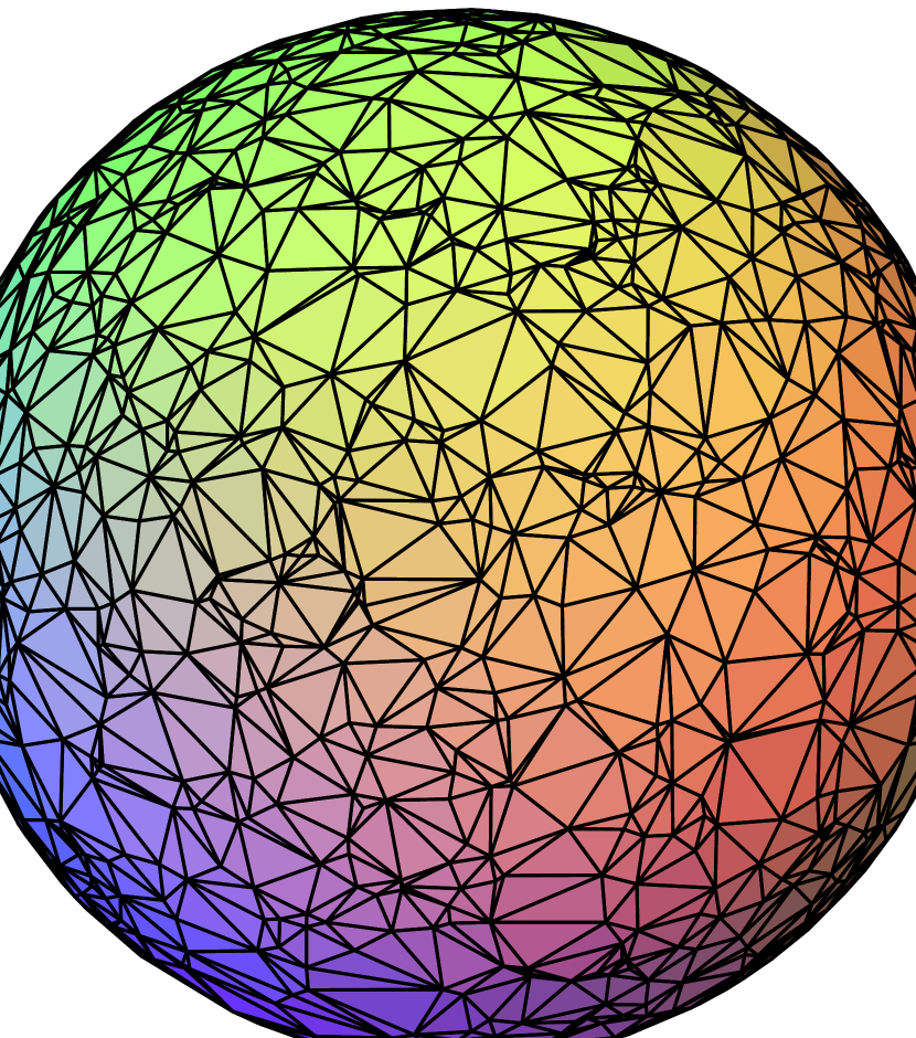
Figure 1: Randomly triangulated sphere with $N_{0}=1500$.

To discretize the global topology of a sphere we used random triangulations that are constructed according to the Voronoi-Delaunay procedure, as described in Ref. [12]. In this way we can control the influence of the special vertices of non-regular triangulations. A sample random triangulation with $N_{0}=1500$ vertices is shown in Fig. 1. For spherical topologies we have the Euler relations $N_{0}-2=N_{1}/3$, $N_{0}-2=N_{2}/2$, and $2N_{1}=3N_{2}$, where $N_{0},N_{1}$, and $N_{2}$ denote the number of sites, links and triangles, respectively. In random triangulations the number of nearest neighbors $q$ varies, theoretically, between 3 and $\infty$. For a finite number of vertices the total number of links is, of course, bounded from above, and in the practical realizations we typically find a maximal coordination number of about $q_{\rm max}\approx 10-13$, depending on the lattice size. Due to the global constraint on $N_{0}$ and $N_{1}$, the average number of nearest neighbors in each realization is given by $\bar{q}=6(1-12/N_{0})$. For our largest realizations with $N_{0}=17\,498$ the probability distribution $P(q)$ of the coordination numbers $q$ is plotted in Fig. 2.

3 FINITE-SIZE SCALING

The previously used methods of Ref.[4, 5, 6] to extract $\gamma_{\rm str}$ are plagued by inconsistencies, as has been discussed in our earlier work [8]. There we also suggested an alternative method to determine the string susceptibilities. For the easier digestion of the present article we recapitulate here only the important points. From the partition function (1) one can easily compute the derivative

$$\frac{\partial\ln Z}{\partial\hat{A}}=-a\lambda+\frac{1}{\hat{A}}(\hat{R}^{2}-1),$$ (7)

where

$$\hat{R}^{2}:=a\langle\sum_{i}R_{i}^{2}\rangle=a\langle\sum_{i}\delta_{i}^{2}/A_{i}\rangle$$ (8)

is the scaled total curvature squared. By inspecting (1) one can then show that $\hat{R}^{2}=\hat{R}^{2}(\hat{A},N_{1})$ depends only on $N_{1}$ and the dimensionless parameter $\hat{A}$.

By comparing with (5) and (6) one expects that for large $N_{1}$ the finite part of $\hat{R}^{2}$ can be expanded into power series,

$$\hat{R}^{2} = b_{1}\hat{A}+b_{0}+b_{-1}/\hat{A}+\dots\qquad(\hat{A}\gg 1),$$ (9)

$$\hat{R}^{2} = b^{\prime}_{-1}/\hat{A}+b^{\prime}_{0}+b^{\prime}_{1}\hat{A}+\dots\qquad(\hat{A}\ll 1),$$ (10)

with

$$b_{1}=-a(\lambda_{R}-\lambda),\quad b_{0}=\gamma_{\rm str}-2\qquad\qquad\qquad\qquad~{}~{}~{}(\hat{A}\gg 1),$$ (11)

and

$$b^{\prime}_{-1}=S_{c},\quad b^{\prime}_{0}=\gamma_{\rm str}^{\prime}-2,\quad b^{\prime}_{1}=-a(\lambda_{R}-\lambda)-b\qquad(\hat{A}\ll 1).$$ (12)

Since the functional form is the same in the two limits (the omitted terms $+\dots$, however, are different), in the following we shall sometimes drop the prime at the coefficients $b_{i}$.

Let us first recall the scaling Ansatz of Refs. [5, 6] where one considers first a power-series expansion of $\hat{R}^{2}(\hat{A},N_{1})$ in $N_{1}$. In Refs. [5, 6] actually $N_{2}$ is used instead of $N_{1}$, but this is trivial because for any compact triangulation we have the fundamental relation $3N_{2}=2N_{1}$. Moreover, and conceptually more important, their expansion of $\hat{R}^{2}$ is not done at fixed $\hat{A}$, but at a fixed discretization scale set by the average triangle area $a_{0}\equiv A/N_{2}$ through the dimensionless parameter $\hat{a}_{0}\equiv a_{0}/a$:

$$\hat{R}^{2}(\hat{a}_{0},N_{2})=N_{2}c_{0}(\hat{a}_{0})+c_{1}(\hat{a}_{0})+c_{2}(\hat{a}_{0})/N_{2}+\dots.$$ (13)

The coefficients $c_{i}(\hat{a}_{0})$ are thus defined in the thermodynamic (infinite area) limit. This expansion is not based on any ab initio calculations, but has to be justified a posteriori by the simulation results. In a second step the coefficients $c_{i}$ are expanded in Refs. [5, 6] into a power series in $\hat{a}_{0}$ as

$$c_{0} = c_{0}^{(0)}+\hat{a}_{0}c_{0}^{(1)}+\dots,$$ (14)

$$c_{1} = c_{1}^{(0)}+\hat{a}_{0}c_{1}^{(1)}+\dots,$$ (15)

$$c_{2} = \!\!(c_{2}^{(0)}+\hat{a}_{0}c_{2}^{(1)}+\dots)/\hat{a}_{0},$$ (16)

and the continuum limit is taken by sending the discretization scale to zero, $\hat{a}_{0}\longrightarrow 0$. A comparison with (9) then yields $b_{1}=c_{0}^{(1)},b_{0}=c_{1}^{(0)}$, and $b_{-1}=c_{2}^{(0)}$. Note, that in order to make contact with the continuum result of eq. (6), $c_{2}$ needs to start with a divergent term $\propto 1/\hat{a}_{0}$. Only in the combined limit $N_{2}\longrightarrow\infty,\hat{a}_{0}\longrightarrow 0$, this makes sense. But because $\hat{a}_{0}$ is fixed, and not $\hat{A}$, effectively there is no control of the crossover from strong $R^{2}$-gravity scaling behavior ($\hat{A}\ll 1$) to the weak $R^{2}$-gravity scaling behavior ($\hat{A}\gg 1$). If one takes first the thermodynamic limit in (13) then one always obtains the values of the coefficients $c_{i}$ in the limit $\hat{A}=N_{2}\hat{a}_{0}\gg 1$, hence for weak $R^{2}$-gravity. This means, $c_{1}^{(0)}=\gamma_{\rm str}-2$, and $c_{2}\longrightarrow 0$, but one has to be careful to make the system size always large enough to reach this limit. If one truncates the fit at some suitable value of $N_{2}$ to explore the region where $\hat{A}\ll 1$, then the continuum limit can only be taken at finite $N_{2}$. Because the results of Ref. [6] were obtained for very small $N_{2}$, finite-size effects can become important. Even worse, because the coefficients $c_{i}^{(j)}$ in the expansion (15) are constants, how can $c_{1}^{(0)}+2$ change from $\gamma_{\rm str}$ to $\gamma_{\rm str}^{\prime}$, as is claimed in Ref. [6]? These subtleties make it appear very unlikely that one can unambiguously extract $\gamma_{\rm str}^{\prime}$ in this way.

We therefore suggested in Refs. [7, 8] a new approach which is in spirit much closer to the continuum analysis of Ref. [3] as it uses $\hat{A}$ as the distinguishing control parameter between weak and strong $R^{2}$-gravity. Expanding $\hat{R}^{2}(\hat{A},N_{2})$ at constant $\hat{A}$ we obtain

$$\hat{R}^{2}(\hat{A},N_{2})=N_{2}d_{0}(\hat{A})+d_{1}(\hat{A})+d_{2}(\hat{A})/N_{2}+\dots.$$ (17)

The next step is to expand the coefficients $d_{i}$ as a power series in $\hat{A}$. The coefficient $d_{1}$ carries all the necessary information to extract the string susceptibilities. A comparison with (9) and (10) yields for weak $R^{2}$-gravity

$$d_{1}(\hat{A})=b_{1}\hat{A}+\gamma_{\rm str}-2+{\cal O}(1/\hat{A})\qquad(\hat{A}\gg 1),$$ (18)

and for strong $R^{2}$-gravity

$$d_{1}(\hat{A})=S_{c}/\hat{A}+\gamma_{\rm str}^{\prime}-2+b^{\prime}_{1}\hat{A}+{\cal O}(\hat{A}^{2})\qquad(\hat{A}\ll 1).$$ (19)

If we plot $d_{1}$ versus $\hat{A}$ we thus expect to see a linear behavior for very large $\hat{A}$, and a divergent behavior for small $\hat{A}$, from which we can extract $\gamma_{\rm str}$ as well as $\gamma_{\rm str}^{\prime}$. The appearance of the classical action in (19) is easy to understand. Actually, for any regular triangulation with coordination number $q$ of arbitrary topology we find from the Euler relation $\delta_{i}=4\pi(1-g)/q$, and $A_{i}=A/q$, therefore $aR^{2}=a\sum\delta_{i}^{2}/A_{i}=16\pi^{2}(1-g)^{2}/\hat{A}=S_{c}/\hat{A}$. For small $\hat{A}$ this will be the dominant term.

As far as the determination of $\gamma_{\rm str}$ is concerned ($\hat{A}\gg 1$), the difference between our method and that of Ref. [5] appears as a subtle interchange of the order in which the thermodynamic and continuum limits are taken. We first take the continuum limit ($N_{2}\longrightarrow\infty$) for fixed $\hat{A}$, and then the thermodynamic limit ($\hat{A}\longrightarrow\infty$), whereas in (13) first the thermodynamic limit is taken for fixed $\hat{a}_{0}=\hat{A}/N_{2}$, ($N_{2}\longrightarrow\infty$, $\hat{A}\longrightarrow\infty$) and then the continuum limit ($\hat{a}_{0}\longrightarrow\infty$) is performed. For $\gamma_{\rm str}^{\prime}$ our procedure is basically the same as before (again with fixed, but now very small $\hat{A}$), whereas the procedure of Ref. [6] exhibits the problems already mentioned earlier.

Because $\hat{R}^{2}$ in (17) becomes infinite in the continuum limit $N_{2}\longrightarrow\infty$, it was suggested to add a non-scale invariant part $q_{ij}^{\alpha}$ to the measure and fine-tune the exponent $\alpha$ such that it cancels the divergent term $d_{0}$. However, a trial simulation showed within error bars no change in the relevant coefficient $d_{1}(\hat{A})$ [8], justifying a posteriori the use of the simple computer measure.

4 SIMULATION

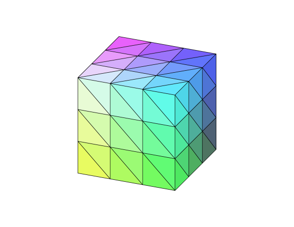
Figure 3: The lattice realization of a spherical topology as the surface of a three dimensional cube with $L=4$, $N_{0}=56,N_{1}=162$, and $N_{2}=108$.

One of the objectives of the present simulations of randomly triangulated spheres was a comparison with previous results for fixed, non-regular triangulations [5, 8]. In these studies the fixed triangulation of the sphere was realized as the surface of a three-dimensional cube where six exceptional vertices have coordination number four, whereas the rest of them have coordination number six, see Fig. 3. The number of vertices is given by $N_{0}=6(L-1)^{2}+2$, where $L$ is the edge length of the cube which in our study [8] was varied from $L=7$ up to $55$.

The randomly triangulated spheres were constructed according to the standard Voronoi-Delaunay procedure [12]. For each lattice size we generated four different realizations (copies) to test how sensitive physical quantities depend on the randomly chosen realizations. In order to allow an easy comparison with our previous results for the triangulated cube, we chose the number of sites again as $N_{0}=6(L-1)^{2}+2$, with $L$ varying from 7, 10, 15, …to 55 in units of 5. This corresponds to $N_{0}=218$ – 17 498 lattice sites, or $N_{1}=648$ – 52 488 link degrees of freedom, or $N_{2}=432$ – 18 252 triangles. To update the link lengths we used a standard multi-hit Metropolis algorithm with a hit rate ranging from 1,…,3. In addition to the usual Metropolis procedure a change in link length is only accepted, if the links of a triangle fulfill the triangle inequalities.

The area $A$ was kept fixed during the update at its initial value $A=\sum_{i}A_{i}=N_{2}/2$ in order to simulate the delta-function constraint in eq. (1). In principle we would need to rescale all links during each link update, amounting in a non-local procedure. However, due to the scaling properties of the partition function, this can be absorbed in a simple scale factor in front of the $R^{2}$-term. To avoid round-off errors we explicitly performed a rescaling after every full lattice sweep. Notice, that our simulation procedure is technically different from the methods employed in Refs. [5, 6].

As in our previous study of a fixed cubic triangulation [8] we ran two sets of simulations. In the first set we employed the method of simulating at constant $\hat{a}_{0}$, using the 8 values of $1/\hat{a}_{0}=2a$ = 10, 20, 40, 80, 160, 320, 640, and 1280. For the last four values we performed in addition to the 11 simulations with $N_{0}=218$ – 17 498 also runs at very small lattice sizes of $N_{0}=26$, 56, 98, and 152, or equivalently $L=3$, 4, 5, and 6, to facilitate the comparison to Ref. [8].

The second set of simulations consists of runs at constant $\hat{A}$ at the 16 values of $\hat{A}=9126/a$ with $a=5$, 10, 20, 40, 60, 80, 120, 160, 240, 320, 480, 640, 800, 960, 1120, and 1280, which cover roughly the range of $\hat{A}=7-1\,800$. Again, for each value of $\hat{A}$, all 11 lattice sizes in the range $N_{0}=218$ – 17 498 were simulated. Here we took the majority of our data, to refine our scaling analyses for $\gamma_{\rm str}$ and $\gamma_{\rm str}^{\prime}$.

For each run on the four copies we recorded between 10 000 and 50 000 measurements of the curvature square $R^{2}\equiv\sum_{i}R^{2}_{i}$ on every second to fourth MC sweep. The statistical errors for each copy were computed using standard jack-knife errors on the basis of 20 blocks. The integrated autocorrelation time $\tau_{R^{2}}$ of $R^{2}$ was usually in the range of 5 – 10. As the final statistical error in the average over the four random lattice realizations we used the standard root mean square deviation (which usually was of about the same size as the statistical error for each realization).

5 RESULTS

5.1 Results at fixed $\hat{a}_{0}$

We first begin with an analysis of the raw data for $\hat{R}^{2}/N_{2}$ which was obtained for the four different realizations of the randomly triangulated sphere in simulations with fixed $\hat{a}_{0}=1/2a$. The data for selected values of $\hat{a}_{0}$ and $N_{2}$ can be found in Table 1. One can see that the difference in $\hat{R}^{2}$ between the copies varies only little with system size and value of $\hat{a}_{0}$ for the system sizes with $L=7$ and $L=15$, where we took 10 000 measurements. Only for the lattice size $L=40$, where we performed 50 000 measurements, the difference between copies is larger than their statistical error. For this lattice size one can also observe that the difference between copies decreases as $\hat{a}_{0}$ tends to zero.

In Table 1 we listed for comparison also our earlier data for $\hat{R}^{2}$ obtained on the surface of a cube. To make the digestion of the data easier, we plotted in Fig. 6 the difference $\Delta\hat{R}^{2}\equiv\hat{R}^{2}_{\rm VD}-\hat{R}^{2}_{\rm cube}$ of the average $\hat{R}^{2}$ on the random Voronoi-Delaunay (VD) spheres and the cubes. We see that the difference $\Delta\hat{R}^{2}$ depends in a quite complicated way on both, $N_{2}$ and $\hat{a}_{0}$. Most disturbing is the observation that the curves seem to converge to zero in the limit $N_{2}\longrightarrow 0$, and not, as one naively would expect, as $N_{2}\longrightarrow\infty$. This shows that even in the thermodynamic limit the curvature data depends on the kind of triangulation, hence is not universal. Even if one sends the discretization scale $\hat{a}_{0}$ to zero, it is far from being obvious that one obtains a unique continuum value for $\hat{R}^{2}$.

To finish our comparison for fixed $\hat{a}_{0}$, we also performed a scaling analysis on the data set obtained on the random sphere according to eq. (13) to obtain an estimate for $\gamma_{\rm str}^{\prime}=2+c_{1}$. As already described in our earlier work [8] one needs to go to very large values of $1/\hat{a}_{0}$ and small values of $N_{2}$ in order to obtain fits of sufficiently high quality. The smallest value of $N_{2}$ we used in this context was $N_{2}=48$. In Table 2 we show the results for $c_{0},c_{1}$, and $c_{2}$ together with the degrees of freedom of the fit ($dof$) and the $\chi^{2}$ value, for our largest values of $a$. The random sphere values utilize the same number of $dof$ as the cube values from Ref. [8] listed above, and below we show the fit results for somewhat more acceptable values of $\chi^{2}$. The results for $c_{1}$ show that, if one uses the same number of data points on the same lattice sizes, then the value of $c_{1}$ on the random spheres is more stable and we get an average $c_{1}=-1.0(1)$, resulting in $\gamma_{\rm str}^{\prime}=1.0(1)$. Also the values for $\chi^{2}$ are smaller, but still not very satisfying. If one discards even more data points on the larger lattices, one finally gets to a more acceptable $\chi^{2}$, but for the cost of having only a few remaining degrees of freedom. The value of $c_{1}$ on the random spheres then seems to approach again the theoretically expected value of $c_{1}=-2$ as $\hat{a}_{0}\longrightarrow 0$ ($a\longrightarrow\infty$), but the whole fitting procedure is still not convincing, see also Fig. 5. The value for $c_{2}\hat{a}_{0}$ comes out almost invariantly close to the expected value of $16\pi^{2}\approx 157.91$, hence cannot serve as a test for the quality of the fits. We conclude again for this section that the estimates for $\gamma_{\rm str}^{\prime}$ obtained in this fashion should not serve as a test for quantum Regge calculus, as was advocated in [5, 6].

5.2 Results at fixed $\hat{A}$

Let us as well begin with a comparison of the values for $\hat{R}^{2}/N_{2}$ obtained for the different realizations of the random sphere which are compiled in Table 3. Noteworthy is that for the larger system sizes the different realizations of the random sphere assume almost the same value within their statistical error, because this time the statistics on the largest lattice size was lower (10 000 measurements) compared to the statistics on the two smaller lattice sizes (50 000 measurements). Also one can observe a tendency that the difference between the copies decreases as $\hat{A}$ decreases. For small $\hat{A}$ the different copies agree with their average within their statistical error.

If one compares now the average of the results for the random spheres with the values obtained for the cube, one observes that the difference in $\hat{R}^{2}$ depends, as one should expect, on the lattice size, such that the difference between the two triangulations decreases as $N_{2}$ increases (which here corresponds to the continuum limit at fixed $\hat{A}$).

However, the difference in $\hat{R}^{2}$ also depends on $\hat{A}$ such that for small $\hat{A}$ the value of $\hat{R}^{2}$ is larger on the cube than on the randomly triangulated sphere ($\Delta\hat{R}^{2}<0$), whereas for large $\hat{A}$ the value of $\hat{R}^{2}$ is smaller on the cube ($\Delta\hat{R}^{2}>0$). This feature can best be inspected in Fig. 6, where we plotted again $\Delta\hat{R}^{2}$ versus $1/N_{2}$. Strictly speaking this shows that $Z$ of eq. (1) and $\hat{R}^{2}$ of eq. (17) depend also on the way the manifold is triangulated, hence $\hat{R}^{2}$ is a non-universal quantity. This time, however, the data clearly shows that, if one sends $N_{2}$ to infinity, one really goes to the continuum limit in which both triangulations should give the same result for $\hat{R}^{2}$.

If this feature remains true for the coefficients $d_{1}$ is far from being obvious. Especially for large $\hat{A}$, i.e., the region which determines $\gamma_{\rm str}$, the values for $d_{1}$ depend on the triangulation, and one can expect universal behavior only for very large lattices. This effect is clearly not visible among the four copies of the random triangulations, therefore we consider them to be the preferred choice of discretization scheme.

As described in Sec. 3, the estimation of the exponents $\gamma_{\rm str}$ and $\gamma^{\prime}_{\rm str}$ from our raw data for $\hat{R}^{2}(\hat{A},N_{2})$ requires a two-step fitting procedure. In the first step one extracts the values of $d_{1}(\hat{A})$ from fits to the FSS behavior according to eq. (17).

In our previus short communication we used linear two-parameter fits, based only on $d_{0}$ and $d_{1}$. Since the curves turned out to be considerably curved we tried this time to account for these corrections to the leading FSS behavior by including also the $d_{2}$ correction of eq. (17), which improved the quality of the fits considerably. The values for the $\chi^{2}/dof$, however, were still considerably larger than one. A closer look at the error bars in $\hat{R}^{2}$ revealed however, that they are probably underestimated, since we had only four random realizations available, and sometimes the thermal average of a single copy was already comparable to the standard deviations over the four copies of the random sphere. This makes it very difficult to decide self-consistently which fit Ansatz is the proper choice. For all values of $\hat{A}$ the quality of the fits can be inspected in Fig. 7. All data points for $d_{0}$, $d_{1}$, and $d_{2}$, together with the value for $\chi^{2}/dof$ and the number of degrees of freedom of the fits are collected in Table 4. The values of $d_{1}$ as a function of all available $\hat{A}$ is shown in Fig. 8.

In the next step the small-$\hat{A}$ and large-$\hat{A}$ regimes have to be treated separately. For small values of $\hat{A}<120$ we fitted $d_{1}(\hat{A})$ according to the Ansatz (19), which yields

$$S_{c} = 151(5),$$ (20)

$$\gamma_{\rm str}^{\prime} = -0.8(5),$$ (21)

with a $\chi^{2}/dof=3$, see Fig. 9. This result is still compatible with the theoretical prediction [3] $S_{c}=16\pi^{2}\approx 158$ and $\gamma_{\rm str}^{\prime}=0$. Compared with our previous results on the triangulated cube ($S_{c}=187(104)$, $\gamma_{\rm str}^{\prime}=5.1(6.6)$) [8], the precision of (20) and (21) is improved. We attribute this not only to the somewhat better scaling behavior on random triangulations and the much higher statistics (we average over 4 realizations, and the runs for each realization have in most cases a 5 times higher statistics than those on the cube), but also and more important to the fact that in the present study we have much more data point available in the interesting small-$\hat{A}$ regime.

However even with the enlarged data set it turned out to be very difficult to control systematic errors caused by the uncertainty of the proper fit Ansatz. For example, we also tested a 2-parameter fit where the classical action was hold fixed at its theoretically predicted value. For this fit we obtained a value of $\gamma_{\rm str}^{\prime}=-1.5(2)$ with almost the same $\chi^{2}/dof\approx 3$. This shows that the systematical errors are larger then the statistical errors, and this is exactly the problem which makes the interpretation of the results so difficult.

For large $\hat{A}$ we can employ Ansatz (18). However, there are only three data points with a sufficiently large $\hat{A}$ available, so no trustworthy estimate can be obtained. A trial linear fit through the last three points yields $\gamma_{\rm str}=-22(2)$ with a total $\chi^{2}=7.4$. It is not clear, however, if we are already in the asymptotic regime, which might set in at much larger $\hat{A}$. Another difficulty is that one is not interested in the slope, but in the intersection of the fit with the $y-$axis, which is far from the location of the points used in the fit and is thus numerically very unstable. As a third large problem we have that the $d_{1}$ estimates from the first fit depend very sensitively on the fit range which is used for the first fits, meaning that one has no good control over the FSS effects.

The systematic uncertainty of our value for $\gamma_{\rm str}$ is therefore hard to estimate, but it is surely an order of magnitude larger than the quoted statistical error. However it is interesting to note that our estimate for $\gamma_{\rm str}$ is much too negative, which is just opposite to what has been claimed in Ref. [5] by using their conceptually different FSS method.

6 CONCLUSIONS

The quantitative difference in $\hat{R}^{2}$ between the non-regular triangulation and the random triangulation of the sphere depends on both, $\hat{A}$ and $N_{2}$. In this way one will obtain on the usually used system sizes different values of $d_{1}(\hat{A})$. The difference seems to be negligible for small values of $\hat{A}$, so that $\gamma_{\rm str}^{\prime}$ can be consistently obtained on both, the cube and the randomly triangulated sphere. However, the difference becomes important for large values of $\hat{A}$, and is thus a potential problem for the determination of $\gamma_{\rm str}$. Because the string susceptibilities are universal quantities, one would expect that the same holds true for the coefficients $d_{1}$. However, then the continuum limit $N_{2}\longrightarrow\infty$ is approached with different speeds on the various lattice realizations.

Random triangulations appear to be a good alternative for topologies where no large regular triangulations exist. They show good scaling behavior, and the differences between different copies of the same area decrease as the system size increases. In this way they can provide a “typical” lattice for the evaluation of expectation values with the partition function of eq. (1).

Our FSS method of fitting at constant values of $\hat{A}$ gives results for $\gamma_{\rm str}^{\prime}$ which are still compatible with the theoretical prediction. In contrast to Ref. [6] we employ a consistent FSS scheme and also much larger lattices. It would be interesting to test if contrary to [6] also for topologies of higher gender the theoretical expectations for $\gamma_{\rm str}^{\prime}$ can be confirmed.

Due to the few data points, only a crude estimate for $\gamma_{\rm str}$ could be obtained which, however, appeared to be too negative compared to the KPZ theory. This is exactly opposite to what has been found in [5] with a different FSS Ansatz. We attribute this discrepancy to their method which, in our opinion [8], bears conceptual problems for large values of $\hat{A}$. It is, however, unclear, if our system sizes are already in the asymptotic scaling regime, so that the potential danger of systematic errors is still very large.

To summarize, we feel that on the basis of all estimates which have been obtained for $\gamma_{\rm str}$ and $\gamma_{\rm str}^{\prime}$ so far there is no contradiction to the theoretical predicted values. This is, however, mainly due to the large uncertainties in the estimated string susceptibilities. Our studies clearly show that on the basis of measurements for the string susceptibilities it is neither fair to claim a success nor a failure of quantum Regge calculus, as has been done before.

Although our FSS method for $\hat{A}$ should conceptually work, it seems very unlikely that the accuracy of the estimates for $\gamma_{\rm str}$ (and the same holds to some extent for $\gamma_{\rm str}^{\prime}$) can be improved in a reasonably sized computer simulation study to serve as a stringent test for the Regge method. The lattice sizes which are needed to reduce corrections to scaling appear to be huge. The problem is that the susceptibility exponents are only subdominant corrections to the leading large area behavior, and as such are very difficult to estimate through FSS studies. It would be definitely more efficient to have a more direct way of measuring $\gamma_{\rm str}$ (or $\gamma_{\rm str}^{\prime}$), as it is done for example in the dynamical triangulation method [1].

	$\hat{R}^{2}(\hat{a}_{0}=1/10,N_{2})/N_{2}$	$\hat{R}^{2}(\hat{a}_{0}=1/160,N_{2})/N_{2}$	$\hat{R}^{2}(\hat{a}_{0}=1/1280,N_{2})/N_{2}$
	$N_{2}=432$, $L=7$
copy 1	0.2483(5)	0.3818(6)	1.3306(6)
copy 2	0.2472(4)	0.3826(7)	1.3315(6)
copy 3	0.2479(5)	0.3831(4)	1.3307(4)
copy 4	0.2474(5)	0.3822(6)	1.3318(6)
average	0.2477(3)	0.3824(3)	1.3311(3)
cube	0.2457(3)	0.3832(6)	1.3315(5)
	$N_{2}=2352$, $L=15$
copy 1	0.2409(2)	0.2516(2)	0.2861(4)
copy 2	0.2403(2)	0.2521(3)	0.2867(5)
copy 3	0.2401(2)	0.2516(3)	0.2875(5)
copy 4	0.2401(3)	0.2517(3)	0.2851(4)
average	0.2404(2)	0.2518(2)	0.2863(6)
cube	0.2352(1)	0.2547(3)	0.2904(5)
	$N_{2}=18252$, $L=40$
copy 1	0.24063(4)	0.24795(8)	0.24975(5)
copy 2	0.24063(6)	0.24798(6)	0.24964(4)
copy 3	0.24001(4)	0.24768(7)	0.24970(6)
copy 4	0.24039(3)	0.24776(5)	0.24960(7)
average	0.24042(15)	0.24784(7)	0.24967(3)
cube	0.23339(3)	0.24789(11)	0.25263(8)

Table 1: Raw data of $\hat{R}^{2}(\hat{a}_{0},N_{2})=a\langle\sum_{i}\delta_{i}^{2}/A_{i}\rangle$ for spherical topology at fixed $\hat{a}_{0}=1/2a$.

$a=1/2\hat{a}_{0}$	$c_{0}$	$c_{1}$	$c_{2}\hat{a}_{0}$	$dof$	$\chi^{2}$
Cube
80	0.2530(4)	-2.0(2)	158.42(6)	3	11.4
160	0.2520(2)	-1.7(6)	158.14(2)	5	16.4
320	0.2522(2)	-1.6(1)	158.04(2)	6	17.0
640	0.2535(2)	-2.1(1)	158.00(1)	6	75.3
random Sphere
80	0.2489(2)	-1.0(1)	158.09(4)	3	7.4
160	0.2486(1)	-0.9(1)	158.02(2)	5	18.5
320	0.2490(1)	-0.9(1)	157.99(2)	6	7.9
640	0.2493(1)	-1.1(1)	157.96(1)	6	21.7
random Sphere with acceptable $\chi^{2}$
80	0.2497(5)	-1.2(2)	158.15(5)	2	3.6
160	0.2498(5)	-1.2(2)	158.07(3)	2	4.7
320	0.2501(7)	-1.3(3)	158.02(3)	2	1.4
640	0.2514(7)	-1.8(3)	157.99(2)	2	1.1

Table 2: Fit results for the Ansatz $\hat{R}^{2}(\hat{a}_{0},N_{2})/N_{2}=c_{0}+c_{1}/N_{2}+c_{2}/N_{2}^{2}$ at fixed $\hat{a}_{0}$. We discarded successively the largest lattices until we obtained a reasonable total $\chi^{2}$ of the fit. The number of degrees of freedom for the fit is denoted by $dof$. For small $\hat{A}$ (i.e. large $a$) we expect $c_{2}\hat{a}_{0}=S_{c}=16\pi^{2}\approx 157.91$.

	$\hat{R}^{2}(\hat{A}=1825,N_{2})/N_{2}$	$\hat{R}^{2}(\hat{A}=114.1,N_{2})/N_{2}$	$\hat{R}^{2}(\hat{A}=14.25,N_{2})/N_{2}$
	$N_{2}=972$, $L=10$
copy 1	0.1913(2)	0.2410(2)	0.2578(2)
copy 2	0.1836(2)	0.2401(2)	0.2576(2)
copy 3	0.1874(2)	0.2415(2)	0.2581(2)
copy 4	0.1897(2)	0.2413(2)	0.2580(2)
average	0.1880(17)	0.2410(4)	0.2579(2)
cube	0.1585(2)	0.2364(2)	0.2594(5)
	$N_{2}=10092$, $L=30$
copy 1	0.2359(1)	0.2469(1)	0.2495(1)
copy 2	0.2359(1)	0.2472(2)	0.2499(2)
copy 3	0.2368(1)	0.2471(1)	0.2497(1)
copy 4	0.2361(1)	0.2469(1)	0.2496(1)
average	0.2362(2)	0.2470(1)	0.2497(2)
cube	0.2261(1)	0.2470(2)	0.2536(3)
	$N_{2}=34992$, $L=55$
copy 1	0.24325(4)	0.24828(6)	0.24950(6)
copy 2	0.24314(5)	0.24829(6)	0.24960(5)
copy 3	0.24325(4)	0.24832(5)	0.24960(4)
copy 4	0.24315(4)	0.24831(5)	0.24950(5)
average	0.24320(3)	0.24830(1)	0.24955(3)
cube	0.23874(5)	0.24848(6)	0.25202(10)

Table 3: Raw data of $\hat{R}^{2}(\hat{A},N_{2})=a\langle\sum_{i}\delta_{i}^{2}/A_{i}\rangle$ for spherical topology at fixed $\hat{A}$.

$\hat{A}$	$d_{0}$	$d_{1}$	$d_{2}$	$\chi^{2}/dof$	$dof$
1825.200	0.24609(7)	-108(2)	89803(6618)	12.4	6
912.600	0.24715(5)	-69(2)	61137(4819)	14.6	6
456.300	0.24773(4)	-43(1)	36802(2976)	9.8	6
228.150	0.24834(6)	-29(2)	24862(3119)	2.2	6
152.100	0.24871(5)	-25(1)	24293(2650)	2.1	6
114.075	0.24882(3)	-19(1)	18817(2387)	3.4	6
76.050	0.24891(3)	-12.2(4)	7396(493)	8.1	7
57.038	0.24892(3)	-9.2(4)	6321(454)	6.6	7
38.025	0.24908(3)	-4.7(3)	4255(305)	5.1	7
28.519	0.24915(2)	-1.6(3)	3468(424)	6.9	7
19.012	0.24932(3)	1.8(5)	3491(4712)	2.4	7
14.259	0.24932(3)	4.9(4)	3337(384)	9.6	7
11.408	0.24941(2)	8.9(3)	2322(376)	1.9	7
9.506	0.24955(2)	11.4(3)	3016(354)	4.9	7
8.148	0.24942(3)	15.7(4)	1450(518)	8.3	7
7.130	0.24963(2)	16.5(4)	3321(351)	3.4	7

Table 4: Fit results for the Ansatz $\hat{R}^{2}(\hat{A},N_{2})/N_{2}=d_{0}+d_{1}/N_{2}+d_{2}/N_{2}^{2}$ at fixed $\hat{A}$. For the six largest $\hat{A}$ values we discarded the smallest lattice size, otherwise we used the fit over all available data points. The number of degrees of freedom for the fit is denoted by $dof$.

Figure 2: The measured probability distribution $P(q)$ of the coordination numbers $q$ for the four realizations of the spherical random lattices with $N_{0}=17\,498$ vertices (corresponding to $L=55$).

Figure 4: Difference $\Delta\hat{R}^{2}/N_{2}$ obtained for various lattice sizes $N_{2}$ on the non-regular cube and the randomly triangulated sphere for the simulations with $2a=1/\hat{a}_{0}=const$. The curves serve only as guides to the eye.

Figure 5: $c_{1}$ plotted vs. $a$, where $c_{1}$ was obtained with eq. (13) on the basis of Table 2. The theory predicts a value of $c_{1}=\gamma_{\rm str}^{\prime}-2=-2$ for the sphere. Noteworthy are the large differences between the random sphere and the cube data, as well as the differences due to different fit ranges.

Figure 6: Difference $\Delta\hat{R}^{2}/N_{2}$ obtained for various lattice sizes $N_{2}$ on the non-regular cube and the randomly triangulated sphere for the simulations with $\hat{A}=const$.

Figure 7: Fits of $\hat{R}^{2}(\hat{A},N_{2})/N_{2}$ to an Ansatz $d_{0}(\hat{A})+d_{1}(\hat{A})/N_{2}+d_{2}(\hat{A})/N_{2}^{2}$, yielding the estimates of $d_{1}(\hat{A})$ of Table 4. These values were then used in the second fits to extract $\gamma_{\rm str}$ and $\gamma_{\rm str}^{\prime}$ displayed in Figs. 8 and 9. The lowest lying data points correspond to the simulations with $\hat{A}=1825.2$. The next data curves correspond, from bottom to top to the $\hat{A}$ values 912.6, 456.3, 228.2, 152.1, 114.1, 76.1, 57.0, 38.0, 28.5, 19.0, 14.3, 11.4, 9.5, 8.1, and 7.1.

Figure 8: Results for $d_{1}(\hat{A})$ vs. $\hat{A}$ together with fits in the regimes $\hat{A}<120$ and $\hat{A}>400$ yielding the estimates $\gamma_{\rm str}^{\prime}=-0.8(5)$ and $\gamma_{\rm str}=-22(2)$, together with the value $S_{c}=151(5)$. The theoretical predictions for spherical topologies are $S_{c}=16\pi^{2}\approx 157.91$, $\gamma_{\rm str}^{\prime}=0$, and $\gamma_{\rm str}=-1/2$.

Figure 9: Blow-up of Fig. 8 for $\hat{A}<120$ yielding the estimate $\gamma_{\rm str}^{\prime}=-0.8(5)$.

References

- [1] H.W. Hamber, Nucl. Phys. B (Proc. Suppl.) 99A, 1 (1991); Nucl. Phys. B (Proc. Suppl.) 25A (1992) 150; J. Ambjørn, Nucl. Phys. B (Proc. Suppl.) 42, 3 (1995); S. Catterall, Nucl. Phys. B (Proc. Suppl.) 47, 59 (1996); D.A. Johnston, Nucl. Phys. B (Proc. Suppl.) 53, 43 (1997).
- [2] V.G Knizhnik, A.M. Polyakov, and A.B. Zamalodchikov, Mod. Phys. Lett. A3, 819 (1988).
- [3] H. Kawai and R. Nakayama, Phys. Lett. B306, 224 (1993).
- [4] M. Gross and H. Hamber, Nucl. Phys. B364, 703 (1991).
- [5] W. Bock and J. Vink, Nucl. Phys. B438, 320 (1995).
- [6] W. Bock, Nucl. Phys. B (Proc. Suppl.) 42, 713 (1995).
- [7] C. Holm and W. Janke, Nucl. Phys. B (Proc. Suppl.) 47, 621 (1996).
- [8] C. Holm and W. Janke, Nucl. Phys. B477, 465 (1996).
- [9] C. Holm and W. Janke, Phys. Lett. B335, 143 (1994).
- [10] C. Holm and W. Janke, Phys. Lett. B390, 59 (1997).
- [11] P. Menotti and P. Peirano, Nucl. Phys. B473, 426 (1996); Nucl. Phys. B (Proc. Suppl.) 53, 780 (1997); Nucl. Phys. B488, 719 (1997); J. Ambjørn, J. Nielsen, J. Rolf, and G. Savvidy, Class. Quant. Grav. 14, 3225 (1997).
- [12] J.L. Meijering, Philips Res. Rep. 8, 270 (1953); N.H. Christ, R. Friedberg, T.D. Lee, Nucl. Phys. B202, 89 (1982); Nucl. Phys. B210 [FS6], 310, 337 (1982); H. Stüben, H.-C. Hege, and A. Nakamura, Phys. Lett. B244, 473 (1990); W. Janke, M. Katoot, and R. Villanova, Phys. Rev. B49, 9644 (1994); W. Janke and R. Villanova, Phys. Lett. A209, 179 (1995).