HIP-1998-47/TH

VORTICES IN EQUILIBRIUM SCALAR ELECTRODYNAMICS

Scalar electrodynamics can be used to investigate the formation of cosmic strings in the early universe. We present the results of lattice Monte Carlo simulations of an effective three-dimensional U(1)+Higgs theory that describes the equilibrium properties of finite-temperature scalar electrodynamics near the transition. A gauge-invariant criterion for the existence of a vortex is used in measuring the properties of the vortex network in the equilibrium state both in the Coulomb and in the Higgs phase of the system. The naive definition of the vortex density becomes meaningless in the continuum limit and special care is needed in extracting physical quantities. Numerical evidence for a physical discontinuity in the vortex density is given.

The traditional picture for defect formation in gauge theories relies on the Kibble mechanism $\!{}^{{\bf?}}$: the effective potential changes shape at the critical point and the field relaxes to different minima in space-time points separated by more than a correlation length. However, strictly speaking this approach can only be applied to transitions in which a symmetry breaks spontaneously, and gauge symmetries cannot be broken $\!{}^{{\bf?}}$. In some cases, e.g. in the electroweak theory, the transition line ends at a critical point after which there is only an analytical crossover between the phases $\!{}^{{\bf?}}$. It is clear that some changes must be made to the picture of defect formation in cases like this.

We will here present the results of the simulations of three-dimensional scalar electrodynamics, i.e. the Abelian Higgs model. The details can be found in the original publications $\!{}^{{\bf?},{\bf?}}$. The theory describes the equilibrium properties of finite-temperature relativistic scalar electrodynamics near the transition $\!{}^{{\bf?}}$, and has the same form as the Ginzburg-Landau theory of superconductivity. We use lattice Monte Carlo simulations to study the behavior of thermally generated vortices, i.e. line-like topological defects, in the two phases of the theory. Similar studies have previously been carried out for the globally symmetric theory using the Langevin equation $\!{}^{{\bf?}}$. Our final aim is to understand non-perturbatively the process of defect formation, but we find it necessary to understand the equilibrium behavior first.

The continuum theory is given by the action

$$S=\int d^{3}x\biggl{[}\frac{1}{4}F_{ij}^{2}+|D_{i}\phi|^{2}+y\phi^{*}\phi+x\left(\phi^{*}\phi\right)^{2}\bigg{]},$$ (1)

where $F_{ij}=\partial_{i}A_{j}-\partial_{j}A_{i}$, $D_{i}=\partial_{i}+iA_{i}$ and $y$ is renormalized in the $\overline{\rm MS}$ scheme at $\mu=1$. In this notation all quantities are dimensionless. If we write $\phi(\mbox{\boldmath$x$})=v(\mbox{\boldmath$x$})\exp[i\gamma(\mbox{\boldmath$x$})]$, the action is invariant under the gauge transformation

$$\gamma(\mbox{\boldmath$x$})\to[\gamma(\mbox{\boldmath$x$})+\theta(\mbox{\boldmath$x$})]_{\pi},\quad A_{i}(\mbox{\boldmath$x$})\to A_{i}(\mbox{\boldmath$x$})-\partial_{i}\theta(\mbox{\boldmath$x$}),$$ (2)

where $[X]_{\pi}\equiv X+2\pi n$ such that $[X]_{\pi}\in(-\pi,\pi]$. The relations of $x$ and $y$ to the parameters of the 4D scalar electrodynamics and superconductors, as well as the determination of the phase diagram, have been discussed elsewhere $\!{}^{{\bf?}}$.

The phase diagram of the system consists of the Coulomb and the Higgs phase. Although a mean-field analysis suggests a symmetry-breaking transition, it turns out that there is, in fact, no local order parameter. The mass of the photon acts as a non-local order parameter, being non-zero in the Higgs phase and vanishing in the Coulomb phase $\!{}^{{\bf?}}$. At small $x$, the transition is of first order as predicted by perturbation theory, but at some critical value of $x$ it becomes continuous $\!{}^{{\bf?}}$ (See Fig. 1a).

For numerical simulations, the theory must be defined on a lattice. We use the non-compact formulation, which means that there is a real number $\alpha_{i}(\mbox{\boldmath$x$})$ corresponding to the continuum gauge field $A_{i}(\mbox{\boldmath$x$})$ on each link $(\mbox{\boldmath$x$},\mbox{\boldmath$x$}+\hat{\imath})$ between the lattice sites. On each site there is a scalar field $\phi(\mbox{\boldmath$x$})=v(\mbox{\boldmath$x$})\exp[i\gamma(\mbox{\boldmath$x$})]$. The lattice analogue of the gauge transformation (2) is

$$\gamma(\mbox{\boldmath$x$})\to[\gamma(\mbox{\boldmath$x$})+\theta(\mbox{\boldmath$x$})]_{\pi},\quad\alpha_{i}(\mbox{\boldmath$x$})\to\alpha_{i}(\mbox{\boldmath$x$})+\theta(\mbox{\boldmath$x$})-\theta(\mbox{\boldmath$x$}+\hat{\imath}).$$ (3)

The parameters appearing in the lattice action differ from the continuum ones, but the relation can be calculated exactly with a 2-loop computation in lattice perturbation theory $\!{}^{{\bf?}}$.

To find the vortices, we define for each link the quantity $\!{}^{{\bf?},{\bf?},{\bf?}}$

$$Y_{(x,x+\hat{\imath})}=[\alpha_{i}(\mbox{\boldmath$x$})+\gamma(\mbox{\boldmath$x$}+\hat{\imath})-\gamma(\mbox{\boldmath$x$})]_{\pi}-\alpha_{i}(\mbox{\boldmath$x$}).$$ (4)

Taking a sum around a closed curve $C$ gives the winding number $n_{C}$:

$$Y_{C}=\sum_{l\in C}Y_{l}\equiv 2\pi n_{C}.$$ (5)

The winding number is a gauge-invariant integer and gives the number of vortices going through the curve $C$ . Using the difference of only the phase angles in Eq. (4) would lead to a non-invariant quantity.

At the mean-field level the notion of a vortex makes only sense in the Higgs phase, but our definition (5) is perfectly valid in all phases and agrees with the intuitive picture of a vortex whenever the bare tree-level potential has a degenerate minimum. We calculate the full path integral numerically using lattice Monte Carlo simulations, which means including the effect of thermal fluctuations to the mean-field picture.

The quantity we are mainly interested in at this stage is the density of thermally generated vortices. The naive way to calculate it is to take the absolute value of the winding number of a single plaquette and measure its expectation value. However, it turns out that in the continuum limit, this quantity approaches a universal quantity $\approx 0.2$, which is independent of the parameters of the theory $\!{}^{{\bf?}}$. The reason is that the winding number of a single plaquette is an ultraviolet quantity, and the ultraviolet behavior of the theory is given by a free massless complex scalar field.

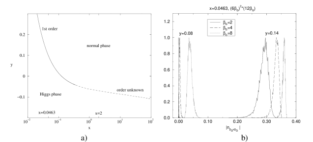
Figure 1: a) The phase diagram of the system. b) The histogram of the volume averages of the winding number of a curve of constant size in physical units at various values of the lattice spacing $a=1/\beta_{G}$. In the continuum limit $\beta_{G}\to\infty$ the distance of the peaks seems to approach a finite value, which is expected to be independent of the regulator.

To obtain a physical quantity, we take a square curve $C$ and keep its size constant in physical units as we approach the continuum limit. While this quantity contains a lot of ultraviolet noise, there is also a physical contribution, and the problem is to extract it. An analogous quantity is $\langle\phi^{*}\phi\rangle$: it diverges in the continuum limit, but the divergent term is constant and can be calculated exactly $\!{}^{{\bf?}}$. The remaining finite part can then be used to probe the phase diagram of the theory. For $\langle|n_{C}|\rangle$ we cannot subtract the divergence exactly, but if it is analytical in the parameters $x$ and $y$ as we expect, the difference in $\langle|n_{C}|\rangle$ above and below the transition line is a physical quantity $\!{}^{{\bf?}}$. Some numerical evidence for that is shown in Fig. 1b.

In practice, it is rather difficult to extract the physical contents of the vortex density defined here. However, it shows that in the continuum limit, more care is needed than simply interpreting the plaquettes with non-zero winding numbers as physical vortices. One has to come up with new observables that give better understanding of the problem before a non-perturbative understanding of defect formation in gauge theories can be obtained.

References

References

- [1] T.W.B. Kibble, J. Phys. A 9, 1387 (1976); W.H. Zurek, Nature 317, 505 (1985).
- [2] S. Elitzur, Phys. Rev. D 12, 3978 (1975); G.F. de Angelis, D. de Falco and F. Guerra, Phys. Rev. D 17, 1624 (1978).
- [3] K. Kajantie, M. Laine, K. Rummukainen and M. Shaposhnikov, Phys. Rev. Lett. 77, 2887 (1996).
- [4] A. Rajantie, Physica B, in press [cond-mat/9803221].
- [5] K. Kajantie, M. Karjalainen, M. Laine, J. Peisa and A. Rajantie, Phys. Lett. B, in press [hep-ph/9803367].
- [6] K. Farakos, K. Kajantie, K. Rummukainen and M. Shaposhnikov, Nucl. Phys. B 425, 67 (1994).
- [7] N.D. Antunes, L.M.A. Bettencourt and M. Hindmarsh, Phys. Rev. Lett. 80, 908 (1998).
- [8] K. Kajantie, M. Karjalainen, M. Laine and J. Peisa, Phys. Rev. B 57, 3011 (1998); Nucl. Phys. B 520, 345 (1998).
- [9] C. Borgs and F. Nill, J. Stat. Phys. 47, 877 (1987).
- [10] M. Laine and A. Rajantie, Nucl. Phys. B 513, 471 (1998).
- [11] J. Ranft, J. Kripfganz and G. Ranft, Phys. Rev. D 28, 360 (1983).
- [12] V.N. Popov, Functional integrals and collective excitations, (Cambridge University Press, Cambridge, 1987).
- [13] G. Vincent, N.D. Antunes and M. Hindmarsh, Phys. Rev. Lett. 80, 2277 (1998); A. Yates and W.H. Zurek, Phys. Rev. Lett. 80, 5477 (1998).