Imaginary chemical potential and finite fermion density on the lattice

Standard lattice fermion algorithms run into the well-known sign problem at real chemical potential. In this paper we investigate the possibility of using imaginary chemical potential, and argue that it has advantages over other methods, particularly for probing the physics at finite temperature as well as density. As a feasibility study, we present numerical results for the partition function of the two-dimensional Hubbard model with imaginary chemical potential.

We also note that systems with a net imbalance of isospin may be simulated using a real chemical potential that couples to $I_{3}$ without suffering from the sign problem.

PACS numbers: 11.15.Ha, 71.10.Fd

1 Introduction

The behavior of fermions in the presence of a chemical potential is relevant to condensed matter physics (Hubbard model away from half-filling) and particle physics (high quark density systems such as the early universe, neutron stars, and heavy-ion collisions). Furthermore, a remarkably rich phase structure has been conjectured for QCD at finite temperature and density [1, 2].

The only reliable non-perturbative approach to QCD is the numerical Monte-Carlo evaluation of the functional integral using a lattice regulator. Unfortunately, standard Monte-Carlo methods become inapplicable at finite quark density, since in the presence of a real chemical potential the measure is no longer positive. One approach to this problem is the “Glasgow method” [3], in which the partition function is expanded in powers of ${\rm e}^{\beta\mu}$, and the coefficients are evaluated by Monte-Carlo, using an ensemble of configurations weighted by the $\mu=0$ action. Simulations using this method have so far given unphysical results, namely, the lattice starts to fill with baryons at a chemical potential well below the expected value of one-third the baryon mass. It seems plausible that this happens because the $\mu=0$ ensemble does not overlap sufficiently with the finite-density states of interest, and so the true effects of quark loops will only be seen at exponentially large statistics [3].

In this paper we look at an alternative: evaluating the partition function at imaginary chemical potential, for which the measure remains positive, and standard Monte-Carlo methods apply. The canonical partition functions can then be obtained by a Fourier transform [4, 5]. Since the dominant source of errors is now the Fourier transform rather than poor overlap of the measure, it seems worthwhile to explore imaginary chemical potential as an alternative to the Glasgow method.

An outline of the paper is as follows. We give criteria that a theory should satisfy in order for Monte-Carlo simulations at finite density to be feasible. We describe a toy model where even-odd effects effects become visible. We find some interesting examples (e.g. QCD at finite isospin density) where lattice simulations are possible. As a feasibility study we perform Monte-Carlo simulations for the two-dimensional Hubbard model with imaginary chemical potential, and find that it is indeed possible to obtain the canonical partition functions at low particle number. At the rather high temperature and low interaction strength that we study, we see no sign of electron pairing.

2 Chemical potential and positivity of the measure

Consider a generic system of fermions $\psi$ and bosons $\phi$, where the fermion Lagrange density is $\bar{\psi}M(\phi)\psi$. On integrating out the fermions, the partition function becomes

$$Z=\int{\cal D}\phi\ {\rm e}^{-S_{bos}(\phi)}\det M(\phi).$$ (2.1)

In order to perform Monte-Carlo simulations it is necessary that the measure be nonnegative, so either we have to restrict ourselves to the cases where $\det M\geqslant 0$, or to treat $\det M$ as an observable. The latter option is usually not viable, as $\det M$ tends to be a rapidly varying function of $\phi$. We will discuss it again at the end of this section.

To guarantee that the measure is positive, we must generally have an even number of flavors, for each of which $\det M$ is real (but not necessarily positive). One situation where $\det M$ is real is when there exists an invertible operator $P$ such that

$$M^{\dagger}=PMP^{-1}.$$ (2.2)

For a Wilson lattice fermion at zero chemical potential this relation holds, with $P=\gamma_{5}$, so any even number of flavors can be simulated by Monte-Carlo. With real chemical potential (2.2) breaks down, but with imaginary chemical potential it is valid, and again simulations are possible for an even number of flavors.

There are more exotic situations where (2.2) holds. For example, consider two-flavor QCD with a finite density of isospin. In this case $M$ has a block-diagonal structure

$$M(\mu)=\left(\begin{array}[]{cc}L(\mu)&0\\ 0&L(-\mu)\end{array}\right),$$ (2.3)

where $\mu$ is the chemical potential for the isospin, and $L(\mu)$ is a Dirac operator for one flavor with chemical potential $\mu$. $L(\mu)$ satisfies $L(\mu)^{\dagger}=\gamma_{5}L(-\mu)\gamma_{5}$, hence Eq. (2.2) is satisfied by setting

$$P=\left(\begin{array}[]{cc}0&\gamma_{5}\\ \gamma_{5}&0\end{array}\right).$$ (2.4)

Here $\det M(\mu)=|\det L(\mu)|^{2}\geqslant 0$. More generally, consider QCD with $N_{f}$ flavors. It has a global vector-like symmetry $G=U(1)_{B}\times SU(N_{f})$, where $U(1)_{B}$ is the baryon number. One may consider a nonzero chemical potential coupled to any generator $T$ of $G$. Then Eq. (2.2) is satisfied for some choice of $P$ if and only if the nonzero eigenvalues of $T$ come in pairs $\lambda,-\lambda$. Thus $\det M$ is real for QCD at nonzero isospin density, but not for nonzero hypercharge density, or baryon number density.

Another case where $\det M$ is real even in the presence of the chemical potential is when there exists an invertible operator $Q$ such that

$$M^{*}=QMQ^{-1}.$$ (2.5)

Examples of this sort are afforded by models with four-fermion interactions, like the Hubbard model and the Gross-Neveu model. There $M$ is a real operator, so $\det M$ is real too. Other examples are gauge theories with “quarks” in the real or pseudoreal representation of the gauge group. Thus $\det M$ is real for $SU(2)$ with quarks in the fundamental representation, or for $SU(3)$ with quarks in the adjoint, even when the chemical potential is nonzero.

In some cases with $\det M$ real but not positive it appears that one can perform simulations by treating the sign of $\det M$ as an observable. The Hubbard model can be treated in this way far below half-filling [6]. This is also the case for the Gross-Neveu model at nonzero chemical potential [7]. Ref. [7] further argues that that $\det M$ is nonnegative for most of the configurations, so one can simply replace $\det M$ with $|\det M|$. In QCD the phase of the determinant contains important physical information, but calculations have been performed without it [8].

3 Imaginary chemical potential

The fact that the fermion determinant for QCD is real in the presence of an imaginary chemical potential $\mu=i\nu$ makes this an attractive option for exploring finite quark density. Simulations with an imaginary chemical potential are more or less equivalent to simulating a canonical ensemble. Indeed, the partition function for imaginary chemical potential

$$Z(i\nu)={\rm Tr}\ {\rm e}^{-\beta\hat{H}}{\rm e}^{i\beta\nu\hat{N}},$$ (3.6)

which is a periodic function of $\nu$ with period $2\pi/\beta$, is the Fourier transform of the canonical partition function

$$Z(N)=\frac{\beta}{2\pi}\int_{0}^{2\pi/\beta}d\nu Z(i\nu){\rm e}^{-i\beta\nu N}.$$ (3.7)

In principle, one can compute $Z(i\nu)$ on a lattice as a function of $\nu$, and then use Eq. (3.7) to obtain the canonical partition function. In practice, this method can work only for low enough $N$, because for large $N$ the integrand in Eq. (3.7) is a rapidly oscillating function, and the error of the numerical integration will grow exponentially with $N$. The method fails completely in the thermodynamic limit $N\rightarrow\infty$. This need not discourage us, however, because in lattice simulations one is always working in a finite and rather small volume. The real question is how high we can push $N$ before the numerical integration in Eq. (3.7) becomes undoable. We will consider the two-dimensional Hubbard model as a testing ground for this approach. Related work has been performed in Ref. [4], but without using the freedom to simulate at any $\nu$ (see below).

Having a positive measure is not the end of the story. In practice we want to be able to use importance sampling to calculate $Z(i\nu)$ with reasonable accuracy. To this end we rewrite $Z(i\nu)$ in the following form:

$${Z(i\nu)\over Z(i\nu_{0})}=\int{\cal D}\phi\ {\rm e}^{-S_{bos}}\det M(i\nu_{0})\,\frac{\det M(i\nu)}{\det M(i\nu_{0})}.$$ (3.8)

Now we treat the ratio of determinants as an observable, and the rest as the measure. A natural worry is that the ratio of determinants could be a rapidly varying function of the bosonic fields $\phi$, which would make Monte-Carlo simulations unfeasible. This is what happens for real chemical potential. However, with an imaginary chemical potential this does not occur. The absolute value of the observable could still be a rapidly varying function. This has to be decided on a case-by-case basis. We will see that for the two-dimensional Hubbard model the ratio of determinants is a slowly varying function of $\phi$, hence $Z(i\nu)$ is computable.

Using (3.8) we can calculate the partition function for a range of $\nu$ around a reference value $\nu_{0}$. It is clear that we can cover the range $\nu=0\ldots 2\pi/\beta$ with a set of “patches” each centered on a different $\nu_{0}$. We can use as many patches as are required, so the measure will always overlap arbitrarily well with the observables.

Some qualitative features of the system can be inferred from the knowledge of $Z(i\nu)$ alone, without performing the Fourier transform. For example, consider a model of interacting fermions on a lattice (the example of the Hubbard model will be discussed further below). At some filling fraction the system may undergo a phase transition to a BCS superconducting phase. In that phase, the system will be populated with Cooper pairs, so the partition function will be dominated by sectors in which the charge is a multiple of 2. This will be clearly visible in $Z(i\nu)$, which will not only be perodic with period $2\pi/\beta$, but acquire a significant subharmonic at period $2\pi/(2\beta)$. This would be a signal that for some range of densities the energy of the system has a minimum when the number of electrons is a multiple of 2.

This can be illustrated by a simple toy model containing a fermion with mass $M_{f}$ and charge 1, and a boson with mass $M_{b}$ and charge 2. If we make $M_{b}$ less than $M_{f}$ then, assuming some very weak charge-conserving interactions that establish equilibrium, states of even charge will be favored.

The free energy is the sum of the fermion and boson contributions,

$$F(\mu,T)=F_{\rm fermion}(M_{f},\mu,T)+F_{\rm boson}(M_{b},2\mu,T),$$ (3.9)

where $F_{\rm fermion}$ and $F_{\rm boson}$ are the free energies of free fermions and bosons, respectively,

$$\begin{array}[]{rcl}F_{\begin{array}[]{c}\hbox{\rm\scriptsize fermion}\\[-3.01389pt] \hbox{\rm\scriptsize boson}\end{array}}(M,\mu,T)&=&\displaystyle\int{d^{3}p\over(2\pi)^{3}}\pm\ln\Bigl{(}1\pm 2\cosh(\beta\mu){\rm e}^{-\beta E(p)}+{\rm e}^{-2\beta E(p)}\Bigr{)},\\[8.61108pt] E(p)^{2}&=&p^{2}+M^{2}.\end{array}$$ (3.10)

Figure 1: Free energy as a function of imaginary chemical potential $\nu$ (left) and log of the canonical partition function as a function of particle number (right) for our illustrative toy model (3.9), with $\beta M_{b}=1$ and $\beta M_{f}=5$.

The pairing of fermions into bosons is clearly visible in $Z(N)$ (Fig. 1), and also directly in $Z(i\nu)$ which is not only perodic with period $2\pi/\beta$, but also approximately periodic with a smaller period $2\pi/(2\beta)$. This is a signal that the energy of a system has a minimum when the number of particles is a multiple of 2. However, to infer the existence of an “unpairing” transition at high chemical potential, a visual inspection of the the plot of $Z(i\nu)$ would not suffice: this information is encoded in the high-frequency behaviour of the Fourier transform of $Z(i\nu)$.

4 Hubbard model with imaginary chemical potential

At densities away from half-filling, the single-flavor Hubbard model has a real but not necessarily positive fermionic determinant [9]. Like QCD, the measure becomes positive at imaginary chemical potential. Since this model is of physical interest and also much less computationally demanding than QCD, it is interesting to use it to study the feasibility of performing simulations with imaginary chemical potential. In fact, the model is so simple that for this initial investigation we were able to dispense with the usual hybrid Monte-Carlo algorithm [9] for evaluating the fermion determinant, and perform the whole calculation with the computer mathematics tool “Mathematica”, using its “Det” function to calculate the fermionic determinants.

Using the formulation described above (see (3.8)), we calculated the partition function as a function of imaginary chemical potential $\nu$. We used a $4^{2}\times 10$ lattice with inverse temperature $\beta=1.5$. (Lower statistics were also gathered on $4^{2}\times 20$, to check that temporal discretization errors were under control.) The results are given in Fig. 2. By particle-hole symmetry, $Z(i\nu)=Z(-i\nu)$, and $Z$ has period $2\pi/\beta$, so we only plot $\nu=0$ to $\pi/\beta$.

Three “patches” were used (see Sect. 3), centered at $\beta\nu_{0}=0,\pi/2$, and $\pi$. At the temperature we study, the error in $Z(i\nu)/Z(i\nu_{0})$ rises rapidly with $|\nu-\nu_{0}|$, so it is crucial to use multiple patches to keep the statistical errors in $Z(i\nu)$ under control. In turn, via the Fourier transform, this controls the errors in $Z(N)$ for $N>0$. In contrast, Ref. [4] only used $\nu_{0}=0$, which is adequate only for the small volume, low temperature, and low particle number ($N\leqslant 2$) they studied.

We then fitted $Z(i\nu)$ to various ansatze, and Fourier transformed them to obtain the canonical partition function $Z_{N}$ (Fig. 3). Even using our very inefficient updating algorithm, we are easily able to to get accurate results up to $N=6$. The error bars reflect the statistical errors in the $Z(i\nu)$ data. We used fit functions of the form $Z(i\nu)=\exp(-a\nu^{2})\times{\rm spline}$.

It has been suggested that at some filling fraction the 2D Hubbard model may exhibit superconductivity, through pairing of the electrons to form Cooper pairs which then condense. Along the lines described in section 3, we would expect such pairing to manifest itself as an even-odd periodicity of $Z_{N}$, leading to a characteristic extra bump in $Z(i\nu)$. At the temperature and coupling that we studied, we see no such evidence of pairing. Obviously it would be very interesting to explore a wider range of parameters. This method might also be suitable for exploring the metal-insulator transition near half-filling, where the sign problem becomes particularly virulent [6]. As noted in Ref. [4], however, it will become much harder to extract the $Z_{N}$ at low temperatures, where the $N=0$ contribution dominates $Z(i\nu)$.

Figure 2: Partition function for 2D Hubbard model as a function of imaginary chemical potential $\nu$, in units of $\pi/\beta$. This is on a $4^{2}\times 10$ lattice, with $\beta=1.5$, hopping term $K=1$, and interaction strength $U=0.1$, following the conventions of Creutz [9].

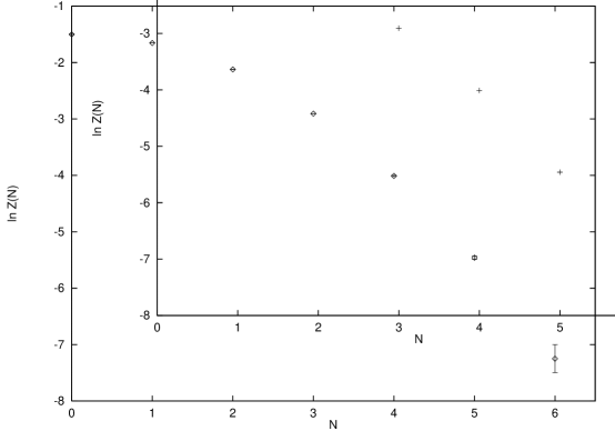
Figure 3: Log of canonical partition function $Z_{N}$ for 2D Hubbard model, obtained by Fourier transform of $Z(i\nu)$ (Fig. 2).

5 Conclusions

Let us conclude with a few remarks concerning the possible utility of imaginary chemical potential in QCD. An imaginary chemical potential does not systematically bias the ensemble to large density, so that to pick out the effect of states of non-zero baryon number density one must rely on fluctuations (which, when they occur, are appropriately weighted by the action). These fluctuations will occur most readily when the temperature is high, and the gap in the baryon number channel is small. And even then one can only realistically hope, on the small lattices likely to be practical, to fluctuate to a few baryons. So a reasonable procedure would seem to be to start with a high temperature and work down, looking for qualitative changes as a function of temperature. In this way, one could realistically hope to use the methods described in this paper to study how properties of the quark-gluon plasma are affected by a net quark density. One could also study the deconfinement crossover, near which the baryons become light, and in particular locate the critical point in the $T-\mu$ plane predicted for two-flavor QCD [2, 10]. All these phenomena are of immediate interest, since they will be explored in the next generation of heavy ion collision experiments.

Another possibility is to work with large numbers of quark species, close to 16, so that the theory is perturbative. Then there is no mass gap to baryons, so fluctuations are cheap, and also the contribution of interest, due to the quarks, is not swamped by gluons. In this case the cancellations may not be so bad even at real chemical potential, and the imaginary chemical potential approach should also work better, since the fluctuations of interest will occur frequently.

Acknowledgements

The research of MGA, AK and FW is supported by DOE grant DE-FG02-90ER40542. MGA is additionally supported by the generosity of Frank and Peggy Taplin.

References

- [1] M. Alford, K. Rajagopal and F. Wilczek, Phys. Lett. B422, 247 (1998), also hep-ph/9804403; R. Rapp, T. Schaefer, E. V. Shuryak and M. Velkovsky, Phys. Rev. Lett. 81, 53 (1998).
- [2] J. Berges and K. Rajagopal, hep-ph/9804233; M. Halasz, A. Jackson, R. Schrock, M. Stephanov, J. Verbaarschot, hep-ph/9804290.
- [3] I. Barbour, S. Morrison, E. Klepfish, J. Kogut, M.-P. Lombardo, Nucl. Phys. B (Proc. Suppl.) 60A, 220 (1998).
- [4] E. Dagotto, A. Moreo, R. Sugar, D. Toussaint, Phys. Rev. B41, 811 (1990).
- [5] A. Hasenfratz and D. Toussaint, Nucl. Phys. B371, 539 (1992).
- [6] S. White, D. Scalapino, R. Sugar, E. Loh, J. Gubernatis, R. Scalettar, Phys. Rev. B40, 506 (1989).
- [7] F. Karsch, J. Kogut, and H.W. Wyld, Nucl. Phys. B280 [FS18], 289 (1987).
- [8] R. Aloisio, V. Azcoiti, G. Di Carlo, A. Galante, A.F. Grillo, Nucl. Phys. B (Proc. Suppl.) 63, 442 (1998).
- [9] M. Creutz, Phys. Rev. D38, 1228 (1988).
- [10] M. Stephanov, K. Rajagopal, E. Shuryak, hep-ph/9806219.