In World Line Path Integral representation Abelian Higgs theories admit a curvature term in the Hamiltonian. Using Monte Carlo simulations we show that the curvature term drives a phase transition at sufficiently strong coupling. In quenched approximation this phase transition is smooth, with implications that the model reduces to a Goldstone theory. Critical properties of the system near the transition are investigated and found to be consistent with mean field behavior.

1 Introduction

In most field theoretic calculations, and in almost all numerical simulations of field theories representations in terms of functional integrals over field variables are used. Yet, for a range of theories another representation, based on the Schwinger proper time formalism, exists and can be utilized for simulations. As Feynman pointed out a long time ago [1] an alternative, quantum mechanical representation of field theories, using world line path integrals (WOLPI) is possible. References to such a representation have appeared sporadically in the literature. De Carvalho, Caracciolo, and Fröhlich showed that the $\phi^{4}$ theory in the $N\rightarrow 0$ limit is equivalent to a self-avoiding random walk. [2] These authors used the WOLPI representation to investigate the question of triviality in scalar field theories. Pisarski considered a theory of paths that, in addition to the standard arc length term also contained a reparametrization invariant curvature term. [3] He showed that the coupling of the curvature term is asymptotically free. Baig, Clua, and Jaramillo [4] simulated a world line using Pisarski’s action. They found a non-singular transition from a random phase to a ”rigid” phase of the world line.

In recent years Strassler used WOLPI representations to calculate complicated vertices in the loop expansion of gauge theories. [5] Awada and Zoller modified Pisarski’s action by adding electromagnetic interactions. [6] These authors investigated the possibility of existence of a phase transition to a new phase of electromagnetic interactions. The nature of their ”rigid” phase was not completely clarified.

In the current paper we will perform a simulation of a world line in the presence of the curvature term and electromagnetic interactions. We will find a phase transition that is equivalent to the Higgs phase transition in the field theoretic representation. Even though no scalar self-interactions are included yet the combination of the curvature term and the electromagnetic interaction generates a self interaction of scalars that induces the transition. In the current paper we study the system in the quenched approximation, or, in other words, in the limit of $N\rightarrow 0.$

The theory we investigate is completely equivalent to a theory of polymers with a particular long range interaction and a stiffness term. As the stiffness increases there is a phase transition to a symmetry breaking phase. In this phase Goldstone bosons, as tadpoles, appear on propagating charge particle lines. As Goldstone bosons appear in all theories with broken continuous symmetries it is quite possible that they have a significance in polymer theories as well.

Before turning to discussing the details of our model we note that simulations in the WOLPI representation have a considerable advantage compared to simulations in the field theoretic functional integral representation, especially at a large number of dimensions, $D$. While the number of computations in field theoretic simulations increases as $L^{D}$, where $L$ is the linear size of the system, even if we do not consider critical slowing down or nonlocal Lagrangians (such as determinants). The required time of simulations in the WOLPI representation increases with the size of the system and the number of dimensions much slower, rather like $L^{2}D$. This is a considerable advantage if $D\geq 3$.

In what follows, we will investigate the Abelian Higgs theory in WOLPI representation. In the next section we derive the general form of the theory and motivate the introduction of the curvature term. In Sec. 3 we discuss the results of our Monte Carlo simulations, while in the last section we analyze our findings and discuss possible directions for further investigations.

2 Higgs theory in the WOLPI representation

We will consider an Abelian Higgs theory with $N$ flavors. First we will reformulate this theory in the language of world line path integrals. Then we will discuss the possibility of generalization in the WOLPI representation by introducing a curvature term.

The gauged Higgs action has the following form in the standard field theoretic representation:

$$S=S_{0}+S_{\rm e.m.}+\frac{g}{2}\int d^{D}x[\phi^{\dagger}(x)\phi(x)]^{2}$$ (1)

where

$$S_{0}=\int d^{D}x\left\{-D_{\mu}\phi^{\dagger}(x)D_{\mu}\phi(x)+m^{2}\phi^{\dagger}(x)\phi(x)\right\}.$$ (2)

and

$$S_{\rm e.m.}=\frac{1}{4}\int d^{D}xF_{\mu\nu}(x)F_{\mu\nu}(x).$$ (3)

Here, as usual, the covariant derivative, $D_{\mu}$, is defined as $D_{\mu}=\partial_{\mu}-ieA_{\mu}(x).$ The electromagnetic field tensor is $F_{\mu\nu}(x)=\partial_{\mu}A_{\nu}(x)-\partial_{\nu}A_{\mu}(x).$ The complex scalar field, $\phi$, has $N$ flavors. Here, and in what follows, flavor indices are suppressed.

Our first step is to integrate out the scalar field from the theory. This can be done after introducing the source, $j(x)$, for the composite operator $\phi^{\dagger}(x)\phi(x)$. Using such a source the partition function can be written as

$$Z=\exp\left\{\frac{g}{2}\int d^{D}y\frac{\delta^{2}}{\delta j(y)^{2}}\right\}\int d\phi(x)dA_{\mu}(x)\exp\left\{iS_{0}+iS_{\rm e.m.}+i\int d^{D}xj(x)\phi^{\dagger}(x)\phi(x)\right\}$$ (4)

The above transformation leads to a Gaussian form in the scalar field. At this moment this procedure seems to be fairly formal, due to the complicated dependence of the action on the source function, $j(x)$. Soon we will see, however, that the theory can be transformed to a more manageable form.

After the Gaussian integration over the scalar field we obtain

$$Z=\exp\left\{\frac{g}{2}\int d^{D}y\frac{\delta^{2}}{\delta j(y)^{2}}\right\}\int dA_{\mu}(x)\exp\left\{\frac{1}{4}F_{\mu\nu}F_{\mu\nu}\right\}\frac{1}{{\rm DET}^{N}}$$ (5)

The determinant, DET=$\det\left[D_{\mu}^{2}+m^{2}+j(x)\right]$, is dependent on the external fields $A_{\mu}$ and $j$. Its logarithm can be written in the path integral form [5]

$$\log{\rm DET}=-\int_{0}^{\infty}\frac{{\rm d}T}{T}\int dx_{\mu}(t)\exp\left\{-\int_{0}^{T}d\tau\left[\frac{x^{\prime 2}+m^{2}}{2}-iex^{\prime}\cdot A[x(\tau)]+j[(x(\tau)]\right]\right\},$$ (6)

where the boundary conditions for the quantum mechanical path integral are $x(T)=x(0)$ and the integration is to be performed over all possible path with the above boundary conditions.

The propagator of a scalar particle can also be written in a functional integral form of the above type. We obtain

$$\Delta(x_{1}-x_{2})=\exp\left\{\frac{g}{2}\int d^{D}y\frac{\delta^{2}}{\delta j(y)^{2}}\right\}\int dA_{\mu}(x)\exp\left\{\frac{1}{4}F_{\mu\nu}F_{\mu\nu}\right\}\frac{\Delta_{A,j}(x^{(1)},x^{(2)})}{{\rm DET}^{N}},$$ (7)

where

$$\Delta_{A,j}(x^{(1)},x^{(2)})=\int_{0}^{\infty}{\rm d}T\int dx_{\mu}(t)\exp\left\{-\int_{0}^{T}d\tau\left[\frac{x^{\prime 2}+m^{2}}{2}-iex^{\prime}\cdot A[x(\tau)]+j[(x(\tau)]\right]\right\},$$ (8)

The propagator depends on background fields $A_{\mu}(x)$ and $j(x)$. In (7) the boundary conditions are $x(0)=x^{(1)}$ and $x(T)=x^{(2)}$.

The expression for the partition function and the propagator can be further simplified and the formal functional differentiations with respect to source $j(x)$ and functional integration over the electromagnetic field can be calculated. This can be done after expanding $DET^{N}$ in a power series of $N$. Then the derivative, $\int d^{D}y\delta^{2}/\delta j(y)^{2}$ simply generates a contact term of $\int_{0}^{T_{i}}d\tau_{i}\int_{0}^{T_{j}}d\tau_{j}\delta^{D}[x(\tau_{i})-x(\tau_{j})]$ in the action. After integrating over the electromagnetic field one obtains the following representation in Euclidean metric

$$Z = \sum_{n=0}^{\infty}\frac{N^{n}}{n!}\int_{0}^{\infty}\prod_{i=1}^{n}\int_{0}^{\infty}\frac{dT_{i}}{T_{i}}\int dx_{\mu}^{(i)}(\tau_{i})\exp\Bigg{\{}-\sum_{i=1}^{n}\int_{0}^{T_{i}}d\tau_{i}\frac{x^{(i)^{\prime}2}+m^{2}}{2}$$ (9)

$$- \frac{e^{2}}{2}\sum_{i,j}^{n}\int d\tau_{i}d\tau_{j}x^{(i)^{\prime}}_{\mu}(\tau_{i})x_{\nu}^{(j)^{\prime}}(\tau_{j})D_{\mu\nu}\left(x^{(i)}(\tau_{i})-x^{(j)}(\tau_{j})\right)$$

$$- \frac{g}{2}\sum_{i,j}^{n}\int d\tau_{i}d\tau_{j}\delta\left(x^{(i)}(\tau_{i})-x^{(j)}(\tau_{j})\right)\Bigg{\}},$$

where $D_{\mu\nu}(x-y)$ is the $D$-dimensional photon propagator. The physical interpretation of this form is as follows. The theory describes the dynamics of closed interacting world lines such that the electromagnetic interaction appears as a long range current-current type interaction between bits of the world line. The scalar self-interaction results in a contact term. This is also a long range interaction in polymer physics because faraway segments along the polymer interact with each other. At infinite coupling (Ising model) this contact term will generate a self-avoiding walk. Note that both types of path-path interactions appear as interactions between different paths and as self-interactions of paths, as well. Our model is completely equivalent to a polymer, albeit with the unusual electromagnetic (current-current) interaction.

The term resulting from the scalar self interaction is well known in polymer physics. [7] It can be rewritten as

$$S_{\rm scalar}=\frac{g}{2}\int d{\bf r}\,[c({\bf r})]^{2},$$ (10)

where $c({\bf r})$ is the polymer density function

$$c({\bf r})=\int d\tau\,\delta[{\bf r-x}(\tau)].$$ (11)

In polymer physics (10) is the first nontrivial term of a virial-expansion in terms of the polymer density. [7]

An expression for the scalar propagator can be found in a manner, very similar to that of the partition function. Using (7) and (8). after manipulations, similar to the ones used for the calculation of the partition function, the propagator can be brought to a form, similar to (9). We only present the form of the propagator in the limit $N\rightarrow 0$ as in the current paper we will not go beyond the quenched approximation. We obtain

$$\Delta(x_{1}-x_{2}) = \int_{0}^{\infty}dT\int dx_{\mu}(\tau)\exp\Bigg{\{}-\int_{0}^{T}d\tau\frac{x^{{}^{\prime}2}+m^{2}}{2}-\frac{1}{2}\int_{0}^{T}d\tau_{1}d\tau_{2}$$ (12)

$$\times \left[e^{2}\,x^{{}^{\prime}}_{\mu}(\tau_{1})x_{\nu}^{{}^{\prime}}(\tau_{2})D_{\mu\nu}\left(x(\tau_{1})-x(\tau_{2})\right)+g\delta\left(x(\tau_{1})-x(\tau_{2})\right)\right]\Bigg{\}},$$

where the world line $x_{\mu}(\tau)$ satisfies the constraint $x(0)=x_{1}$, and $x(T)=x_{2}$.

The expression (12) contains divergences. These divergences partly come from the delta function of the contact density self-interaction. That term can be regularized by smearing the delta function to a ball of radius $a$. Similarly, the electromagnetic propagator appearing in the action becomes singular at short distances. Awada and Zoller recommended a regularization by separating the paths for $x(\tau_{1})$ and $x(\tau_{2})$ in the electromagnetic interaction term. [6]. Such a regularization is gauge invariant. If the two trajectories are shifted away from one another along the principal normal then one can show that one introduces a finite renormalization of the form $\pm e^{2}\int d\tau/R$, where R is the radius of curvature. In fact, if we do not insist on splitting the curves along the principal normal, but say at a fixed angle from it, then we can get an arbitrary finite contribution of the form

$$\delta S_{\rm curv}=\chi\int\frac{d\tau}{R},$$ (13)

where $\chi$ is an arbitrary constant satisfying $|\chi|<e^{2}$. This is exactly the type of term proposed by Pisarski [3]. This term is reparametrization and scale invariant. Since certain regularization procedures require its presence (albeit with a fixed regularization dependent finite coefficient) there is no reason why it would be forbidden in the world line representation. As derived from the field theoretic representation its value is finite, fixed, and regularization dependent. In what follows we will include such a term in the action, with an arbitrary coefficient, and prove that its presence induces a phase transition in Abelian Higgs theories. Thus, the theory we study is a generalization of the standard Higgs Lagrangian, but one that is admissible in the WOLPI representation.

The reparametrization invariance can be used to fix the world line such that $|x^{\prime}(\tau)|=1$. We will use this gauge in the rest of this paper. We will also introduce the effective mass, $M=(x^{{}^{\prime}2}+m^{2})/2$.

3 Simulations

To perform simulations we are required to discretize the world line, replacing it by a finite number of straight segments. Unlike in standard simulations, in which fields are defined at discretized points of the spacetime, it is not necessary to tie WOLPI representation simulations to a lattice. In fact, there is a definite advantage of allowing the vertices of the world line to move to arbitrary points of ${\cal R}^{D}$. The critical region of our investigations will be at large values of the curvature term and of the electromagnetic coupling. At these values the curvature of the world line is small and the lattice approximation that allows the change of direction of the world line only by $\pi/2$ is very crude. Fortunately, there is no real numerical advantage of working on a lattice either. The most computer intensive part of evaluating the action is the calculation of the electromagnetic energy that is not very strongly dependent on whether the vertices are on ${\cal Z}^{D}$ or on ${\cal R}^{D}$.

There is another, even more important, advantage of not doing the simulations on a lattice. As (12) shows the calculation of the propagator requires integration over the length of the world line. On a lattice, with a fixed number of segments, the length of the world line is fixed. Our Monte Carlo procedure that allows points on the world line move freely automatically averages over the length of the world line to some extent.

As we mentioned earlier, there is a significant advantage of world line simulations compared to simulations involving fields. When one simulates a local field theory on a lattice, even if critical slowing down effects, getting more and more significant at large lattice sizes, are not considered, the number of floating point operations per update increases as a multiple of $L^{D}$, where $L$ is the linear size of the lattice and $D$ is the number of spacetime dimensions. World line simulations with long range forces (such as an electromagnetic interaction) require $L^{2}D$ elementary calculations (update $L$ points which all interact with all other $L$ points). Thus, when $D\geq 3$ there is a definite advantage of performing simulations in the world line representation.

The discretized form of the action, appropriate for numerical simulations, is as follows:

$$Z=\int\prod_{i=1}^{L}d{\bf r}^{(i)}\exp\left\{-\sum_{i=1}^{L}[M\,|\Delta{\bf r}^{(i)}|+\chi\sin(\theta_{i,i+1}/2)]-\frac{e^{2}}{2}\sum_{i,j}^{L}\frac{\Delta{\bf r}^{(i)}\cdot\Delta{\bf r}^{(j)}}{({\bf r}^{(i)}-{\bf r}^{(j)})^{2}+a^{2}}\right\},$$ (14)

where $\theta_{i,i+1}$ is the angle between the $i$th and $(i+1)$st segments of the world line, and $\Delta{\bf r}^{(i)}={\bf r}^{(i+1)}-{\bf r}^{(i)}$. We use here the Feynman gauge for the electromagnetic propagator. The cutoff distance, $a$, sets the length scale and as such it can be chosen arbitrarily to be 1. Then the effective mass, $M$, is chosen to be low enough, corresponding to a small value of $a$. In most of the simulations we used $M=0.2$. The self-interaction term of the scalars is not expected to affect the phase transition significantly because the combination of the electromagnetic term and of the curvature term generate an effective scalar self-interaction anyway. Therefore, in the current paper, we set $g=0$ and defer the investigation of the case of $g>0$ to a future publication.

In our simulations a sweep constituted of changing the coordinates of all $L$ vertices, one by one. We restricted these changes within a fixed radius and used the Monte Carlo method to accept or reject individual moves. The radius of allowed moves was varied to achieve a 50% acceptance ratio.

We performed simulations both at $D=3$ and $D=4$. We also used two different forms for the electromagnetic propagator. First we used both at $D=3$ and at $D=4$ the $D=4$ inspired form of $D_{\mu\nu}(x)=\delta_{\mu\nu}/(x^{2}+a^{2})$, as given in (14). The special property of this propagator that it is scale invariant in every dimension, at least at vanishing cutoff parameter, $a$. Then at $D=3$ we also tried the physically correct cutoff electromagnetic propagator, $D_{\mu\nu}(x)=\delta_{\mu\nu}/\sqrt{x^{2}+a^{2}}$. Finally, we simulated both closed loops and open world lines. The phase structure of the system was largely independent of the choice of dimension or that of the electromagnetic interaction. This fact also points into the direction that the transition is related to the breaking of the same symmetry, charge conservation, irrespective of the details of the interaction.

We simulated both closed and open world lines. Closed world lines correspond to the condensate or propagator corrections on the gauge boson, while open world lines simulate the propagator of charged particles. Rather than fixing the endpoints of the world line at $x_{1}$ and $x_{2}$, we allowed the endpoints of open world lines to move freely. This allowed us to measure the probability distribution of $R$, the end-to-end distance of the world line, which is proportional to the propagator. This distribution plays a significant role in the analysis of the nature of the phase transition.

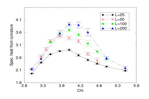
Figure 1: The dependence of the specific heat, $\partial^{2}Z/\partial\chi^{2}$ on $\chi$ in the critical region at fixed $e^{2}=0.5$. The purpose of the connecting lines is to guide the eye.

The salient feature of simulations is the developing of a significant maximum in the specific heat, $d^{2}Z/d\chi^{2}$, as a function of $\chi$ and fixed $e$, provided the fixed value of $e$ is sufficiently large. The peak also appears in $d^{2}Z/de^{2}$ at fixed, sufficiently large $\chi$ and increasing e. The height of the peak increases rapidly as a function of the number of segments on the world line, $L$, which controls the size of the system. This is a telltale sign of a second order phase transition. Fig. 1 shows the dependence of specific heat of the curvature term on $\chi$ at fixed $e^{2}=0.5$ and $L=$25, 50, 100, and 200 in the critical region. There is a clear evidence for a second order phase transition at around $\chi_{c}=4$. Note the the difference between the curve at $L=25$ on one hand and the curves at larger $L$ on the other hand. This difference suggests that at $L=25$ large $L$ asymptotic scaling laws, used to extract critical behavior, are not always applicable.

By changing $e^{2}$, as well, and by exchanging the role of $\chi$ and $e^{2}$ one can arrive at the phase diagram sketched in Fig. 2. It is interesting to note that the phase transition occurs always at non-vanishing value of both $\chi$ and of $e^{2}$. Thus, the smooth transition observed by Baig et al. [4] in the absence of electromagnetic interactions is distinct from the phase transition we observe.

To understand the nature of this phase transition it is very instructive to observe the characteristic shapes of world lines in various regions of the phase diagram. These shapes are shown in the appropriate regions of the phase diagram in Fig. 2. Below the phase transition (low $\chi$) the world line strongly resembles a random walk. In fact, it is easy to prove that the world line must follow a random walk at vanishing $e^{2}$ no matter how large the curvature term is.This is true for every polymer with an action containing finite range correlations only. [7] At low $e^{2}$ and high $\chi$ it does not look like a random walk only because of limitations in the length of the path as the effective radius of the random walk becomes larger than $L$. Above the phase transition segments of the world line running in opposite directions pair up to form tree diagrams of a theory with paired double lines. This signals the appearance of bound states of zero mass (vanishing total four momentum) and the same quantum number as the charge operator, formed from bilinears of the charged scalars. This is clearly a Goldstone boson. As the Goldstone boson makes its appearance at the phase transition, the phase transition should be a Higgs-type transition.

Figure 2: The phase diagram of the system in the $\chi-e^{2}$ plane. Characteristic shapes of world lines are shown in various regions.

Before we were able to check our hypothesis concerning the nature of the phase transition we needed to solve a crucial problem affecting simulations near or above the critical line. By employing our local update procedure the convergence of simulations for the specific heat became intolerably slow at $\chi\sim\chi_{c}$ or $\chi>\chi_{c}$. This phenomenon is very reminiscent to the one observed in simulations of random surfaces by Ambjorn, Bialas, Jurkiewicz, Burda, and Petersson [8] who observed that above a critical point baby universes form and are very stable against local changes. They would not change over enormous computer simulation times. The use of global changes, amputation and reattachment of baby universes was required to speed up the algorithm.

We are faced with a very similar problem in our world line simulations. The limbs of tree diagrams formed from particle-antiparticle bound states are extremely stable against local changes. Therefore, we introduced two global moves that can change these configurations effectively. Both of these moves intend to change configurations with paired world lines. Therefore, after every sweep of local updates, we employ these moves to a randomly chosen pair of points, that are far away from each other along the world line, but are closer than a pre-determined distance in the ${\cal R}^{D}$ target space.

The global moves we employ are: 1) bending the world line along the connecting line of two points that are close in ${\cal R}^{D}$ space but widely separated along the world line, 2) amputating the part of the world line beyond a similarly selected pair of points and attaching the amputated part to an other pair of randomly selected similarly close pair of points. These moves satisfy the detailed balance requirement and were constructed in a way that they would not change the action by a large amount so that their acception rate would not be intolerably low. The result of the introduction of these global moves was a substantial increase in the speed of convergence of simulations near or above the phase transition. Without the introduction of global moves it is practically impossible to perform simulations at a world line length $L\geq 100$. It is quite possible that other, more sophisticated global moves would further speed up the the algorithm.

Though the shapes of the world line in the two phases shown in Fig. 2 give a telltale sign of the nature of the phase transition, we need to find quantitative support for our hypothesis of symmetry breaking transition. We found that the best measure describing the nature of the strong coupling phase is the end-to-end correlation function of open world lines. As we mentioned before, when we simulate open world lines then instead of fixing the endpoints to calculate the scalar propagator between a pair of points we allow the endpoint to move freely. By this we are able to measure the relative probability of propagation to points at varying distance.

The distribution of the end-to-end distance at $e=0$ is Gaussian. This is true for the distribution of random walks with arbitrary finite range correlations in the action. [7] For such random walk like paths one has the following form for the distribution of the end-to-end distance, $R$

$$P(R)\sim\exp\left\{-\frac{3R^{2}}{2b^{2}L}\right\},$$ (15)

where $b$ is the effective bond length. At $e^{2}=0$ there is only a “nearest neighbor” correlation along the world line. At finite values of $e^{2}$ this distribution is expected to be renormalized and the $L$ factor in the denominator of the exponent of (15) replaced by a factor of $L^{2\nu}$, where $\nu$ is the correlation length exponent. On the contrary, in a phase dominated by a bound state, one expects the end-to-end distance distribution to be independent of the length of the world line. The segment of the world line between the two end points corresponds to the propagation of the charged scalar particles. The finiteness of this segment proves a bound system. This can be contrasted to the doubled up part of the world line that corresponds to the propagation of massless bound state formed from the scalars and propagates freely to a distance of $O(L)$. In particular, if the potential creating the bound state is bounded, then the single particle propagator decreases exponentially at large distances, such as

$$P(R)\sim\exp\left\{-MR\right\},$$ (16)

where $M$ is the energy gap. For an unbounded, confining potential the propagator decreases faster for large distances. In that case, the decrease of the propagator at large distances is faster than exponential.

Fig. 3. shows the dependence of the propagator, $P(R)$, on $R$ at $\chi=5.0$ and $e^{2}=0.5$, in the broken phase. The distributions for $L=25$, 50, 100, and 200 perfectly track each other and at distances $R>2$ are in complete agreement with an exponential dependence on $R$ (a straight line in the figure, having a logarithmic scale). The transition between the two regimes is illustrated on the plot, in Fig. 4, of $\langle R^{2}\rangle$, where $R$ is the end-to-end distance, for $L=25$, 50, 100, and 200, as a function of $\chi$, at fixed $e^{2}=0.5$. Clearly, below the phase transition ($\chi_{c}\simeq 4.2$) there is a strong dependence on $L$, that can be well fitted to the formula

$$\langle R^{2}\rangle\sim A+B\ L^{2\nu}$$ (17)

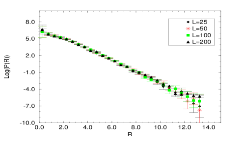
Figure 3: The dependence of the propagator, $P(R)$, on $R$ at $\chi=5.0$ and $e^{2}=0.5$, in the broken phase. A straight line corresponding to an exponential dependence of P(R) on R gives a perfect fit at $R>2$.

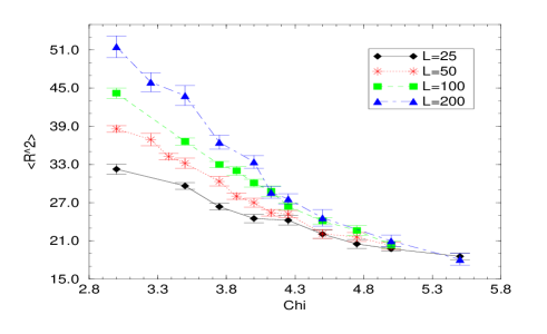
Figure 4: The square of the end-to-end distance as a function of $\chi$ in the critical region at fixed $e^{2}=0.5$. The purpose of the connecting lines is to guide the eye.

that follows from a renormalized version of (15), while above the phase transition $\langle R^{2}\rangle$ is smaller and independent of $L$. Omitting data at $L=25$ the fit to (17), assuming the mean field (free) value, $\nu=1/2$, at every value of $\chi<4.25$, is perfect. Using the dependence of the coefficient $B$ in (17) using a linear extrapolation, we can extrapolate to a critical point at $\chi_{\rm crit}=4.4\pm 0.3$. Unfortunately, the closer one goes to the critical point the less data at smaller values of $L$ fit the asymptotic formula (17). Therefore, a better estimate for the critical point can be obtained if we use only data at the highest values of $L$, $L=200$ and $L=100$. The difference of $\langle R^{2}\rangle$ is plotted for these values in Fig. 5. These data do not allow for any meaningful fit of the critical behavior, but provide a rough estimate of the critical point as $\chi_{\rm crit}=4.2\pm 0.4$.

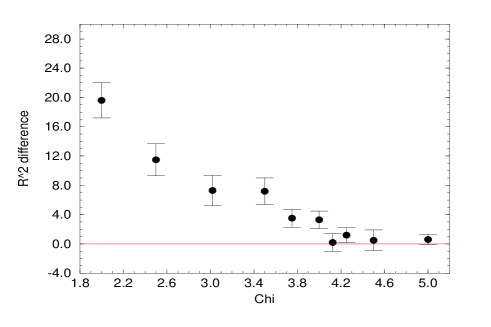
Figure 5: The difference of the squares of the end-to-end distances at $L=200$ and $L=100$ as a function of $\chi$.

In a similar manner we measured the propagator of the particle-antiparticle system. Since particle-antiparticle propagators are non-vanishing to distances of $O(L)$ the normalization of these propagators depends on the value of $L$.

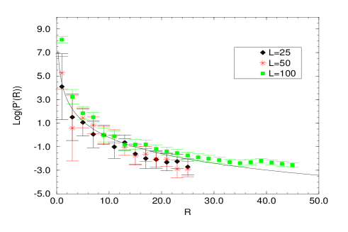
Figure 6: The dependence of the propagator of the particle-antiparticle system, $P^{\prime}(R)$, on $R$ at $\chi=5.0$ and $e^{2}=0.5$, in the broken phase. As these propagators have an infinite range and extend to $R\sim L$, they are normalized to equal values at $R=9$. The curve is $-2\log(R)$, corresponding to a massless free particle.

Therefore, we plot these propagators in Fig. 6 using a normalization so that they coincide at the arbitrarily chosen point, $R=9$. Using this normalization the propagators show a remarkable agreement with each other and with the curve $P^{\prime}(r)\simeq 1/r^{2}$, the true scalar propagator (up to logarithmic corrections) of a zero mass particle in four dimensions. These particle-antiparticle propagators can be obtained either from open or from closed loops. Closed loops also correspond to corrections to the gauge boson propagator. Having a zero mass pole at $N>0$ they would generate a non-vanishing mass to the gauge propagator in agreement with the Higgs mechanism.

There are various other ways to determine the critical properties of the system. One is using finite size scaling. The behavior of specific heat near the phase transition is [9]

$$C(\chi)=A+B\left\{[\chi-\chi_{\rm max}(L)]^{2}+FL^{-2/\nu}\right\}^{-\alpha/2},$$ (18)

where $\alpha$ is the specific heat exponent, $\nu$ is the correlation length exponent, and $\chi_{c}(N)$ is the maximum of the specific heat curve and it depends on the size of the system as

$$\chi_{\rm max}(L)=\chi_{c}-c\,L^{-1/\nu}.$$ (19)

Alternatively, if the critical exponent $\alpha$ vanishes, as it does in the mean field approximation, then the singularity of the specific heat is logarithmic, as in

$$C_{\chi}=A+B\log\left\{[\chi-\chi_{\rm max}(L)]^{2}+FL^{-2/\nu}\right\}.$$ (20)

Our fits to the specific heat are consistent with the mean field prediction of a logarithmic singularity of the specific heat, but a small value of the exponent $\alpha$ cannot be excluded. Our data are insufficient to make any meaningful prediction for the correction term, $FL^{-2/\nu}$. We could, however, analyze the dependence of $\chi_{\rm max}(L)$ on $L$ according to (19). Using $\nu=1$, we found that $\chi_{\rm crit}=4.15\pm 0.08$, in agreement with our earlier estimate of the critical point from the end-to-end distance distribution.

Our understanding of the world line configurations of Fig. 2 is now the following: In the Higgs phase corrections to the Higgs propagator contain tadpole diagrams. These tadpole diagrams are generated by the interaction of Higgs particles with Goldstone bosons and Goldstone bosons with each other. As we simulate a single world line only (quenched approximation) only tree diagram tadpoles formed from the Goldstone boson propagator appear. We expect that in the approximation, $g>0$, loop diagrams formed from the Goldstone boson would also make their appearances. The expected effect of having a finite number of flavors, $N$, will be discussed in the next section.

4 Conclusions

In the world line path integral representation the Abelian Higgs theory admits the addition of a curvature term to the Hamiltonian. We showed that the addition of such a term with a sufficiently large coupling generates a second order phase transition from the symmetric phase to a broken phase in which particle-antiparticle bound states can propagate to large distances or, in other words, form zero mass (Goldstone) bosons. The critical properties of the system were investigated and were found, with admittedly large errors, to be in agreement with a mean field behavior. As the curvature term appears in a natural manner in the world line representation (certain ultraviolet regularizations require its appearance) we expect that this theory is in the same universality class as the Higgs theory in the field theoretic representation, in which there is no term in the Lagrangian, equivalent to the curvature term. This identification of the universality classes leads, however, to several natural questions that need be answered to fully understand the significance of our results:

1. In four dimensions the Higgs phase transition should be of first order, as it was shown a long time ago by Coleman and Weinberg. [10] Why do we find a second order phase transition in our simulations?

2. In a Higgs theory the charge symmetry is broken. Thus, the single charged particle and particle-antiparticle sectors should mix with each other. Yet we find separate asymptotic states in these sectors.

3. In a Higgs theory no zero mass particles should exist, as the Goldstone boson is absorbed by the longitudinal component of the massive gauge boson. What is the reason than that we still seem to see a zero mass asymptotic state?

The short answer to questions 1) and 3) is that the discrepancy is the consequence of the quenched approximation that we use in the current paper. In the $N\rightarrow 0$ limit closed scalar loops do not make their appearances. These scalar loops are needed to generate a mixing between particle-antiparticle states and gauge bosons. At $N>0$ closed scalar loops appear. In a simulation they should be produced freely, as states with a finite number of loops give a finite contribution to the partition function. In paired up lines, formed from particle-antiparticle states, the line pair would go over into a pure gauge state with high probability. This is tantamount to spontaneously forming closed bosonic loops. Particle-antiparticle systems then cannot propagate freely any more, but after a finite distance they annihilate and form, along with virtual gauge boson states, the massive longitudinal component of the physical gauge boson. Our conclusion is then that the $N\rightarrow 0$ limit is a Goldstone limit of the Higgs theory. The theory should then be in the universality class of a pure scalar theory. That theory has a second order phase transition with mean field exponents.

The second question in the above list concerns the mixing of states with different particle numbers. Note that even in the field representation such a mixing occurs only if we shift the fields and expand around the correct vacuum. In the absence of such a shift the Goldstone boson can only appear in the $Q=0$ sector, i.e. in the sector of the broken generator. While expanding around the false vacuum the charge operator, $Q$, seems to be conserved. In the world line representation the value of the charge operator on a surface equals the number of world lines crossing the surface. Clearly, unless we allow the creation of world lines from vacuum, charge is formally conserved. Putting it slightly differently, if we use eigenstates of the charge operator, such as the states built from a definite number of world lines, then we do not see the breaking of charge symmetry, but we still see the appearance of Goldstone bosons signaling the phase transition.

Another way to argue for the second order nature of the phase transition in the $N\rightarrow 0$ limit is as follows. If the electromagnetic interactions of the single world line are sufficiently strong they provide a scalar self-interaction that breaks the symmetry. The first order transition in the Coleman-Weinberg mechanism is generated by gauge loops. The logarithmic divergence of the effective potential in one loop order comes from the two gauge boson intermediate state diagram in particle-antiparticle scattering. [10] In the absence of this diagram and similar diagrams the Coleman-Weinberg mechanism does not operate.

We can only speculate why the nonzero value of the curvature term is required for the phase transition. Clearly, in forming the zero mass bound states the electromagnetic energy competes with the entropy, as the particle and antiparticle have much larger phase space if they are not tied together into a bound state. Apparently, in the absence of the curvature term the electromagnetic energy can never win this competition. The introduction of the curvature term effectively decreases the entropy as world lines become straight. The straight particle and the antiparticle world lines only need to be made parallel (involving a finite number of degrees of freedom) to form the bound state. This is a competition that the electromagnetic energy can easily win.

It is clear from the above discussion that it would be interesting to perform simulations at $N>0$, where the phase transition should switch to first order. We conjecture that the $g\rightarrow 0$ limit does not influence the nature of the transition. This conjecture should also be checked against simulations. In the future we intend to perform appropriate simulations to investigate these effects.

Acknowledgments: The authors are indebted to Professor A. Baig for discussions and for an exchange of codes. Discussions with Drs. I. Shovkovy and L.C.R. Wijewardhana are also greatfully acknowledged. This work was supported in part by the U.S. Department of Energy under grant DOE DE-FG02-84ER-40153 and by a grant of the Ohio Supercomputer Center where most of the calculations were performed.

References

- [1] R. Feynman, Phys. Rev. 80, 440 (1950);
- [2] C.A. De Carvalho, S. Caracciolo, and J. Fröhlich, Nucl. Phys B215 [FS7] 209, (1983);
- [3] R. Pisarski, Phys. Rev. D34, 670 (1986);
- [4] M. Baig, J. Clua, and A. Jaramillo, hep-lat/9607039; M. Baig and J. Clua, Nucl. Phys. Proc. Suppl. 53, 728 (1997)
- [5] M. J. Strassler, Nucl. Phys. B385, 145 (1992);
- [6] M. Awada and D. Zoller, Int. J. Mod. Phys. A9 4077 (1994); ibid. Phys. Lett. B325, 119 (1994);
- [7] ”The Theory of Polymer Dynamics,” M. Doi and S.F. Edwards, Clarendon Press, Oxford 1986;
- [8] J. Ambjorn, P. Bialas, J. Jurkiewicz, Z. Burda, and B. Peterson, Phys.Lett. B325 337-346, (1994);
- [9] M.E. Fisher and A.E. Ferdinand, Phys. Rev. Lett 28 832, (1967); A.E. Ferdinand and M.E. Fisher, Phys. Rev. 185 832, (1969); K. Binder, Physica, 62, 508 (1972);
- [10] S. Coleman and F. Weinberg, Phys. Rev. D8, 1888 (1973).