1 Introduction

Among the different attempts to construct a viable theory of quantum gravity, Euclidean quantum gravity is one of few that allows for non-perturbative studies using numerical methods. In the Euclidean approach one works with a functional integral over Euclidean metrics $g$ weighted by the Einstein-Hilbert action:

$$S_{E}([g_{ab}])\;=\frac{1}{16\pi G}\;\int_{\cal M}\;{\rm d}^{D}\xi\;\sqrt{g(\xi)}(R-2\Lambda),$$ (1)

where $G$ is the Newton’s gravitational constant, $\Lambda$ the cosmological constant and $R$ the scalar curvature of the metric $g_{ab}$ on the space-time manifold ${\cal M}$.

Simplicial gravity, or dynamical triangulations, is a regularization of this model where the integration over metrics is replaces by all possible gluings of $D$-simplexes into closed simplicial manifolds [2, 3]. In three dimensions the regularized partition function becomes

$$Z(\mu,\kappa)\;=\;\sum_{T\in{\cal T}}\;\frac{1}{C_{T}}\;{\rm e}^{\textstyle-\mu N_{3}+\kappa N_{0}}$$ (2)

where ${\cal T}$ denotes an appropriate ensemble of three-dimensional simplicial manifolds, $C_{T}$ is the symmetry factor of a triangulation $T$, $N_{i}$ is the number of $i$-simplexes in the triangulation, and $\mu$ and $\kappa$ are coupling constants related to the cosmological and the inverse Newton’s constant, respectively.

As it stands the model Eq. (2) needs not to be well defined for any value of the couplings; unless the sum over manifolds is restricted in some way it is not convergent [3]. The same is true in two dimensions where, without the restriction to triangulations of fixed topology, the number of triangulations is not exponentially bounded as a function of volume — a necessary condition for convergence of the sum. In three dimensions the situation is even worse, there is no proof that even restricted to fixed topology the sum is convergent. The existence of an exponential bound is, however, strongly supported by numerical simulations for an ensemble of spherical combinatorial triangulations [4, 5].

The model Eq. (2) has been studied extensively using numerical simulations [4, 5, 6, 7]. It has a discontinuous phase transition at a value of the inverse Newton’s constant $\kappa\approx 3.8$, separating a strong-coupling (small $\kappa$) crumpled phase from a weak-coupling branched polymer phase. The crumpled phase is dominated by triangulations of almost zero extension; characterized by few vertexes connected to a large portion of the triangulation and has a internal fractal dimension $d_{H}=\infty$. This excludes any sensible continuum limit in this phase as the distance between two points will always stay at the Planck scale. The branched polymer phase is, on the other hand, dominated by essentially ”one-dimensional“ triangulations — bubbles glued together along small necks into a tree-like structure — with fractal dimension two.

Little attention has been paid so far to the ensemble of triangulations included in the partition function Eq. (2), although in two dimensions it is well known that while different ensembles yield the same continuum theory [8] the finite-size effects depend strongly the type of triangulations used. It has been shown that the less restricted the triangulations are — the larger the ensemble of triangulations is — the smaller the finite-size effects are [9, 10]. This result can be understood intuitively as, for a given volume, with a larger triangulation-space it is easier to approximate a particular fractal structure. This is especially important as in simulating models of dynamical triangulations the geometric finite-size effects usually dominate.

Simulations of simplicial gravity in dimensions larger than two have until now used exclusively combinatorial triangulations. In a combinatorial triangulation each $D$–simplex is uniquely defined by a set of ($D+1$) vertexes, i.e. it is combinatorially unique. In this paper I explore a different ensemble of triangulations, degenerate triangulations, defined by relaxing this restriction and allow distinct simplexes defined by the same set of vertexes. This allows, for example, two vertexes connected by more than on edge and simplexes that have more than one face in common. I retain, on the other hand, the restriction that for every simplex all its ($D+1$) vertexes should be different, i.e. I exclude degenerate simplexes. As the ensemble of degenerate triangulation includes combinatorial triangulations as a subclass, it is obviously larger and as I will demonstrate in this paper this leads to smaller finite-size effects, just as in two dimensions. Apart from this, using degenerate rather than combinatorial triangulations does not seem to change the phase structure of the model Eq. (2); as the coupling constant $\kappa$ is varied I observer a discontinuous phase transition separating a crumpled phase from a branched polymer phase.

The paper is organized a follows: In Section 2  I define the different ensembles of three-dimensional triangulations to be considered and discuss some practical aspects such as ergodicity of the algorithms used in the simulations and the possible problem with pseudo-manifolds. In Section 3  I describe the numerical setup and compare the efficiency of the simulations and the finite-size effects for the ensembles of degenerate versus combinatorial triangulations. In Section 4  I investigate the phase structure of the model, identify a phase transition and show that it is discontinuous, and explore the different phases. Finally, in Section 5  I discuss the practical consequences of this for further simulations of simplicial gravity.

2 Degenerate triangulations

2.1 Different ensembles of triangulations

The triangulations included in the partition function Eq. (2) are constructed by successively gluing equilateral 3-simplexes (tetrahedra) together along their two-dimensional faces (triangles) into a closed three-dimensional simplicial manifold [2, 3]. Pseudo-manifolds are eliminated from the ensemble by the restriction that the neighborhood of every vertex in the triangulation should be homeomorphic to a sphere. To each tetrahedra there is associated a set of four vertexes, or 0-simplexes; the order of a vertex (or more generally of a sub-simplex) is defined as the number of tetrahedra containing that vertex. A dual graph to a triangulation is defined by placing a vertex in the center of each tetrahedra and connecting vertexes in adjacent tetrahedra together. For a three-dimensional triangulation the dual is a $\phi^{4}$-graph. A triangulation is said to be degenerate if it contains two distinct 3-simplexes, or sub-simplexes, which are combinatorially identical, i.e. defined by the same set of vertexes. A simplex is said to be degenerate if it is defined by a set of vertexes including the same vertex more than once.

By imposing additional restrictions on how the simplexes may be glued together, it is possible to define different ensembles of triangulations. In this paper I will consider two such ensembles; combinatorial and degenerate triangulations. Before discussing these different ensembles in three dimensions, let’s start by describing the corresponding triangulations in the simpler case of two dimensions. Given the definitions above we distinguish among three types of two-dimensional triangulations:

• Combinatorial triangulations : ${\cal T}_{C}$
  In a combinatorial triangulation every triangle, and every edge, is combinatorially distinct, i.e. it is uniquely defined by a set of distinct vertexes. From this it follows that no two triangles have more than one edge in common and a triangle cannot be its own neighbor. The dual graph to a combinatorial triangulation is a $\phi^{3}$-graph, excluding both tadpoles and self-energy diagrams.

• Restricted degenerate triangulations : ${\cal T}_{D_{R}}$
  By allowing distinct triangles (or edges) that are combinatorially equivalent, i.e. defined by the same set of three (two) vertexes, while still excluding degenerate triangles, we define a restricted ensemble of degenerate triangulations, ${\cal T}_{D_{R}}$. This type of triangulations can have vertexes connected by more than one edge, and triangles that have two edges in common. In this case self-energy diagrams are allowed in the dual $\phi^{3}$-graph.

• Maximally degenerate triangulations : ${\cal T}_{D_{M}}$
  Finally, by also allowing degenerate triangles we define an ensemble of maximally degenerate triangulations, ${\cal T}_{D_{M}}$. This ensemble allows self-loops — edges starting and ending at the same vertex — equivalently, both tadpoles and self-energy diagrams are included in the dual $\phi^{3}$-graph.

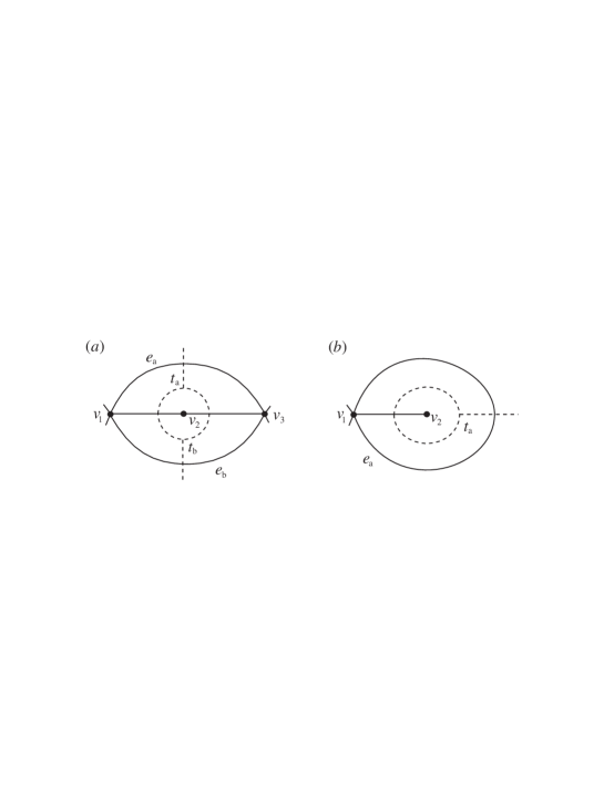
Figure 1: An example of degenerate two-dimensional triangulations. The dashed lines indicate the corresponding dual graphs. In (a) the triangles $t_{a}$ and $t_{b}$ have two edges in common, $\{v_{1},v_{2}\}$ and $\{v_{2},v_{3}\}$ (a self-energy diagram); this type of degeneracy is allowed in restricted degenerate triangulations. In (b) the triangle $t_{a}=\{v_{1},v_{1},v_{2}\}$ is degenerate (corresponds to a tadpole); this is allowed in maximally degenerate triangulations.

Clearly ${\cal T}_{C}\subset{\cal T}_{D_{R}}\subset{\cal T}_{D_{M}}$. I show examples of those different types of degeneracy in Figure 1. As models of pure two-dimensional simplicial gravity defined with those different ensembles can been solved analytically as matrix models, it is known that in all cases they define the same continuum theory [8]. This is, of course, what one would expect based on universality; the different ensembles simply amount to different discretization of the manifolds and the details of the discretization should be irrelevant in the continuum limit. This is true even if the triangulations are restricted even further and only minimal curvature fluctuations of $\pm 1$ are allowed (including only vertexes of order 5, 6 and 7) [10]. But, as mentioned in the Introduction, the finite-size effects do depend on the ensemble used, in particular they increase as more restrictions are placed on the triangulations [9, 10].

Analogous to two dimensions, by imposing the appropriate restrictions in three dimensions I defined the corresponding three different ensembles of triangulations. By allowing distinct but combinatorially equivalent non-degenerate simplexes, I define an ensemble of restricted degenerate three-dimensional triangulations. Compared to combinatorial triangulations, in this ensemble two tetrahedra may be glued together along more than one of their faces. I show examples of this in Figure 2.

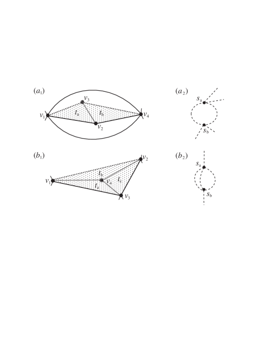
Figure 2: Two examples of degeneracy allowed in three-dimensional degenerate triangulations. Figures ($a_{2}$) and ($b_{2}$) show the corresponding dual $\phi^{4}$-graphs. In both examples there are two distinct but combinatorially equivalent tetrahedra $s_{a}$ and $s_{b}$, defined by the same set of vertexes $\{v_{1},v_{2},v_{3},v_{4}\}$. In ($a_{1}$) the tetrahedra have two triangles in common, whereas in ($b_{1}$) they share three triangles, in which case the dual graph is a self-energy diagram.

Relaxing these restrictions further and allow degeneracy within the simplexes themselves defines an ensemble of maximally degenerate triangulations, ${\cal T}_{D_{M}}$ This allows, for example, self-loops both in the triangulation and in its dual graph (a simplex that is its own neighbor). Although this type of degenerate triangulations is a priori well defined, my numerical investigation indicates that this ensemble does not lead to a well defined statistical model. I tried to simulate the model Eq. (2) using maximally degenerate triangulations; however, in quasi-canonical simulations (see Section 3) it was not possible to tune the cosmological constant $\mu$ in such a way that the volume fluctuated around a fixed target volume $\bar{N}_{3}$. Regardless of the value of $\mu$ used, in the course of the simulations the volume eventually exploded. This behavior suggests that the numbers of maximally degenerate three-dimensional triangulations grows faster than exponentially with the volume, in which case the partition function Eq. (2) does not converge. In the rest of this paper I only consider the ensemble ${\cal T}_{D_{R}}$, omitting the specification restricted when referring to it.

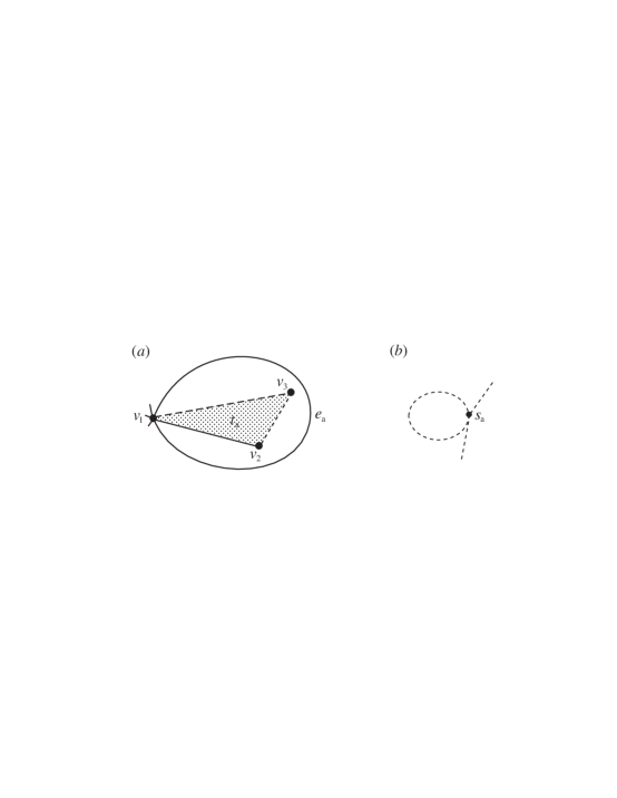
Figure 3: An example of a degenerate simplex, $s_{a}=\{v_{1},v_{1},v_{2},v_{3}\}$, allowed in a three dimensional maximally degenerate triangulation. The edge $e_{a}=\{v_{1},v_{1}\}$ is a self-loop.

2.2 Ergodicity in the updating procedure

Having defined degenerate triangulations, a necessary prerequisite for using them in numerical simulations of simplicial gravity is that there exist a set of ergodic geometric moves which allow us to explore the triangulation-space. For combinatorial triangulations this is provide by the ($p,q$)–moves, a variant of the Alexander moves [11]. In three dimensions the ($p,q$)–moves consist of either inserting or removing a vertex of order four, or replacing a triangle by an edge of order three and vice verse. These moves are depicted in Figure 4. To apply the same set of moves in simulations with degenerate triangulations I have to show that they are also ergodic when applied to the ensemble ${\cal T}_{D}$. To do so it is sufficient to show that every degenerate triangulation can be changed into a combinatorial triangulation using a finite sequence of the ($p,q$)–moves. I distinguish among three different types of degeneracy in restricted degenerate triangulations: combinatorially equivalent tetrahedra, triangles and edges, all of which can be eliminate following the appropriate procedures:

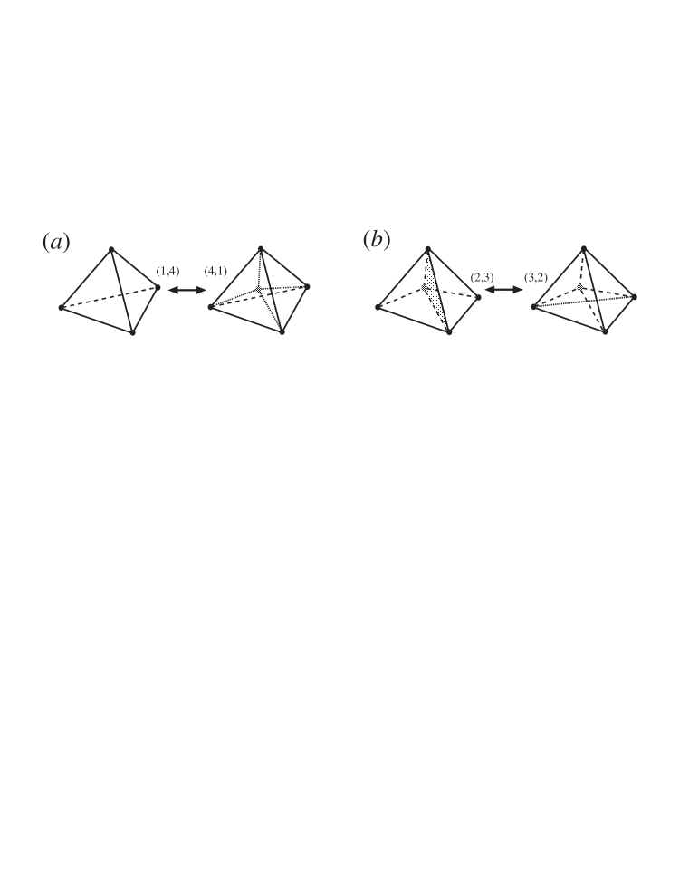
Figure 4: The ($p,q$)–moves in three dimensions: (a) Inserting a vertex and its inverse, deleting a vertex. (b) Replacing a triangle by an edge and vice verse.

• Equivalent tetrahedra:
  In the case of two, or more, tetrahedra defined by the same set of vertexes it is sufficient to insert a vertex (applying move $(1,4)$) into each of those tetrahedra, this will create a set of combinatorially distinct 3-simplexes.

• Equivalent triangles:
  Given two triangles defined by identical set of vertexes I can apply move $(2,3)$ to one of them, i.e. replace that triangle with a new edge. To ensure that the new edge does not result in multiply connected vertexes, and to make sure the move is not rejected by a geometric constraint, prior to using move $(2,3)$ I can apply move $(1,4)$ to both of the tetrahedra containing the triangle in question — the new edge now joins two previously unconnected vertexes.

• Equivalent edges:
  It is slightly more complicated to eliminate a par of distinct edges connecting the same two vertexes. To remove an edge I must apply move $(2,3)$, i.e. replace it with a triangle. This is, however, only possible if the corresponding edge is of order three. To reduce the order of the edge I apply move $(2,3)$ repeatedly to the neighboring triangles. It is possible that some of those triangles could be combinatorially identical; this I eliminate by first applying procedure (b). The remaining triangles can then safely be replaced until the order of the edge is three.

An additional complication that could arise when restrictions on the triangulations is relaxed is the appearance of pseudo-manifolds [2]. In general when gluing $D$–simplexes together into a closed manifold one does not get a simplicial manifold but a pseudo-manifold. A simplicial manifold is defined by the additional requirement that the neighborhood of each vertex is homeomorphic to the $D$–dimensional ball $B_{D}$. As this requirement is trivially satisfied for $D=2$, all degenerate triangulations in two dimensions are automatically simplicial manifolds. It is a priori not clear that in simulating degenerate triangulations in three dimensions, pseudo-manifolds could not be generated — something we would like to avoid.

I observe, however, that in order to generate a pseudo-manifold the ($p,q$)–moves must change the topology of the dual complex to a given vertex $v_{0}$ in the triangulation. By the dual complex I mean the two-dimensional triangulation constructed by connecting by edges the centers of all adjacent tetrahedra containing $v_{0}$. But as the moves only change the triangulation, hence the dual complex, locally they will not change its topology. More precisely, when applying a ($p,q$)–move to a three-dimensional triangulation, degenerate or not, the change in the local neighborhood of each of the vertexes involved in the move can be given in terms of the corresponding two-dimensional ($p,q$)–moves (i.e. inserting/deleting a vertex or flipping an edge) applied to its dual complex. This ensures that the topology of the dual complex is not changed when the move is applied and pseudo-manifolds are not generated.

3 Simulating degenerate triangulations

To study the model Eq. (2) I now turn to numerical simulations. As the ($p,q$)–moves in three dimensions do not preserve the volume of the triangulation the simulations cannot be restricted to the canonical ensemble, contrary to what is possible in two dimensions. In addition, fluctuations in the volume are necessary to maintain ergodicity in the updating procedure. In practice though I perform quasi-canonical Monte Carlo simulations, with almost fixed $N_{3}$, simulating the partition function

$$Z(\mu,\kappa;\bar{N}_{3}) \;=\; \sum_{N_{3}}\;{\rm e}^{\textstyle-\mu N_{3}-\gamma(N_{3}-\bar{N}_{3})^{2}}\;\Omega_{N_{3}}(\kappa),$$ (3)

$$\Omega_{N_{3}}(\kappa) \;=\; \sum_{T\in{\cal T}({N_{3}})}\;\frac{1}{C_{T}}\;{\rm e}^{\textstyle\;\kappa N_{0}}.$$ (4)

Here $\Omega_{N_{3}}(\kappa)$ is the canonical partition function and the quadratic potential term added to the action ensures, for an appropriate choice of the parameter $\gamma$, the necessary fluctuations around a target volume $\bar{N}_{3}$. In simulating degenerate triangulations I found $\gamma\approx 0.001$ to be an appropriate choice. In all cases I simulate an ensemble of spherical triangulations.

From a practical point of view simulating degenerate triangulations is actually simpler than simulating combinatorial triangulations. For the latter the most time-consuming part of the update is the manifold check, i.e. to verify that there exist no sub-simplex in the triangulation combinatorially equivalent to the one created by the move [12]. In three dimensions this check is done both when a triangle is replaced by an edge, and vice verse. This check is not needed for degenerate triangulation; the only geometric check that remains is in replacing a triangle by an edge the two tetrahedra involved must only have one triangle in common. As this check is local the computational effort needed to update a degenerate triangulation is less than for a combinatorial one.

This does not automatically imply that simulations with degenerate triangulations are more efficient. As the ensemble of degenerate triangulations is much larger the corresponding critical cosmological constant $\mu_{c}$ is also larger than for the ensemble of combinatorial triangulations. And as $\mu_{c}$ enters the detail balance condition used in the Metropolis test this in effect reduces the acceptance rate in the updating procedure. To compare the efficiency of simulating the different ensembles I must estimate how fast, measured in CPU-time, independent configurations are generated. I have done this for both ensembles in the crumpled phase, $\kappa=0$. I caution, however, that the comparative efficiency will depend on several factors: the particular implementation of the algorithm, how efficiently the manifold checks are executed, the probability of choosing the different moves, and where in the phase-space the simulations are carried out. In the comparison I use the same program for both types of triangulations, turning on and off the manifold checks, and choose the different moves with equal probability. I measure the CPU-times $t_{s}$ (in ms) it takes to perform one ”sweep“ through the triangulations; a sweep is defined as $\bar{N}_{3}$ attempted local moves, and the auto-correlation times $\tau$ in units of sweeps, measured for the time-series of the energy-density $n_{0}=N_{0}/N_{3}$. Combining $t_{s}$ and $\tau$, I get an estimate of how fast independent configurations are generated:

$${\cal T}_{n_{0}}\;\approx\;\left\{\begin{array}[]{ll}0.43\;N_{3}^{\;2.07}&\mbox{combinatorial,}\vspace{5pt}\\ 230\;\;N_{3}^{\;1.14}&\mbox{degenerate.}\end{array}\right.$$ (5)

For small triangulations, $N_{3}\approx 800$, the effective auto-correlations are comparable for the two ensembles, whereas for larger volumes simulating degenerate triangulations is substantially faster.

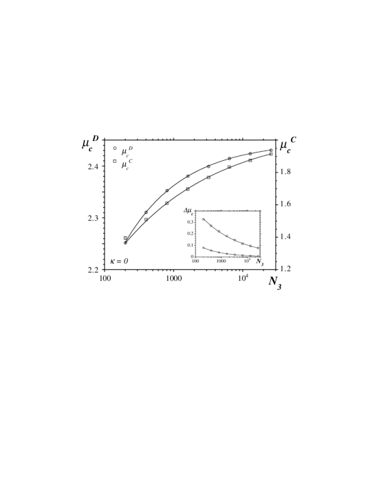
Figure 5: The effective critical cosmological constant $\mu_{c}(N_{3})$, both for an ensemble of degenerate (circles) and combinatorial (diamonds) triangulations. The solid lines are fit to the form: $\mu_{c}(N_{3})=\bar{\mu}_{c}+\beta/N_{3}^{\gamma}$. Insert: The relative deviation from the infinite volume value: $\Delta\mu_{c}=|\bar{\mu}_{c}-\mu_{c}(N_{3})|/\bar{\mu}_{c}$.

The real benefit of using degenerate triangulations comes from the reduction in finite-size effects. This reduction is especially pronounced in the crumpled phase where the internal geometry is dominated by collapsed manifolds. To demonstrate this I measured the volume dependence of the effective critical cosmological constant $\mu_{c}^{D}(N_{3})$ for $\kappa=0$ and for triangulations of volume $N_{3}\lesssim 25000$. This I show in Figure 5. For comparison I include in the figure the corresponding values $\mu_{c}^{C}(N_{3})$ for combinatorial triangulations. For both ensembles $\mu_{c}(N_{3})$ approaches a finite value $\bar{\mu}_{c}$ as the volume diverges; this in turn implies that the canonical partition function $\Omega_{N_{3}}$ is exponentially bounded as a function of volume — an necessary condition for the partition function Eq. (2) to be convergent. I have fitted the data to an assumption of a power-law convergence to an exponential bound (including volumes $N_{3}\geq 400$); this yields:

$$\mu_{c}(N_{3})\;=\;\left\{\begin{array}[]{llll}2.073(21)-3.67(44)\;N_{3}^{\;-0.31(2)},&\chi^{2}=4.0\qquad\mbox{combinatorial,}\vspace{5pt}\\ 2.447(3)\;\;-2.97(29)\;N_{3}^{\;-0.51(2)},&\chi^{2}=0.8\qquad\mbox{degenerate.}\end{array}\right.$$ (6)

For both ensembles the quality of the fit (the $\chi^{2}/{\rm d.o.f}$) is acceptable. This can be compared to a fit to a super-exponential growth of $\Omega_{N_{3}}$, compatible with the assumption $\mu_{c}(N_{3})\approx\alpha+\beta\log N_{3}$, which is definitely ruled out by a very large $\chi^{2}$ value.

There is, however, a marked difference in how fast $\mu_{c}$ approaches its infinite volume value for those two ensembles. This is shown in the insert in Figure 5 where I plot $\Delta\mu_{c}=|\bar{\mu}_{c}-\mu_{c}(N_{3})|/\bar{\mu}_{c}$. Taken at face value, this suggests a reduction of finite-size effects by two orders of magnitude when using degenerate rather than combinatorial triangulations. This huge reduction is though presumable only achieved in the crumpled phase where collapsed manifolds dominate the partition function and the geometric finite-size effects are most pronounced.

4 The phase structure

4.1 Existence of a phase transition

I now turn to the existence of a phase transition in the model as the inverse Newton’s constant $\kappa$ is varied. For combinatorial triangulations it is well established by numerical simulations that the model Eq. (2) has a discontinuous phase transition at $\kappa\approx 3.8$, separating a strong-coupling (small $\kappa$) crumpled phase from a weak-coupling branched polymer phase [4, 5, 6]. As I will demonstrate in this section this is also the case for degenerate triangulations; moreover, the discontinuous nature of the transition is easily observed on triangulations of relatively modest size.

I have simulated the model Eq. (4) for target volumes $N_{3}=200$ to 6400, and for each volume I search for a phase transition in the fluctuations of the energy-density $n_{0}=N_{0}/N_{3}$. A signal for a transition would be a peak in the specific heat:

$$C_{N_{3}}\;=\;\frac{\kappa^{2}}{N_{3}}\;\left(\langle N_{0}^{2}\rangle-\langle N_{0}\rangle^{2}\right).$$ (7)

This is shown in Figure 6 for different target volumes. I did simulations at few values of $\kappa$ around the observed peaks, collecting between two and ten thousand independent measurements, and then used standard multi-histogram methods to interpolate between the measurements. The interpolations is shown as solid lines in Figure 6, the dashed lines indicate the errors.

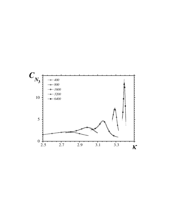
Figure 6: The measured specific heat $C_{N_{3}}$ — the fluctuations in the number of vertexes $N_{0}$ — as the inverse Newton’s constant $\kappa$ is varied. This is for target volume $N_{3}=400$ to 6400. The solid lines are interpolations between measurements, using multi-histogram methods, and the dashed lines indicate the error.

To infer about the nature of the transition I look at the energy-density distribution $\rho(n_{0})$. For sufficiently large target volume this distribution has a well resolved double-peak structure, indicating a discontinuous phase transition. This double-peak structure is observed already on volumes $N_{3}>1600$. I show an example of the measured energy distributions in Figure 7 (thin lines) for the three largest volumes I studied, together with fits to a form composed of two Gaussian peaks (thick lines):

$$\rho(n_{0})\;=\;a_{1}\;{\rm e}^{\textstyle-c_{1}(b_{1}-n_{0})^{2}}+a_{2}\;{\rm e}^{\textstyle-c_{2}(b_{2}-n_{0})^{2}}.$$ (8)

Each distribution is normalized by the height of the peaks and the value of $\kappa$ is chosen so that the two peaks are of equal height.

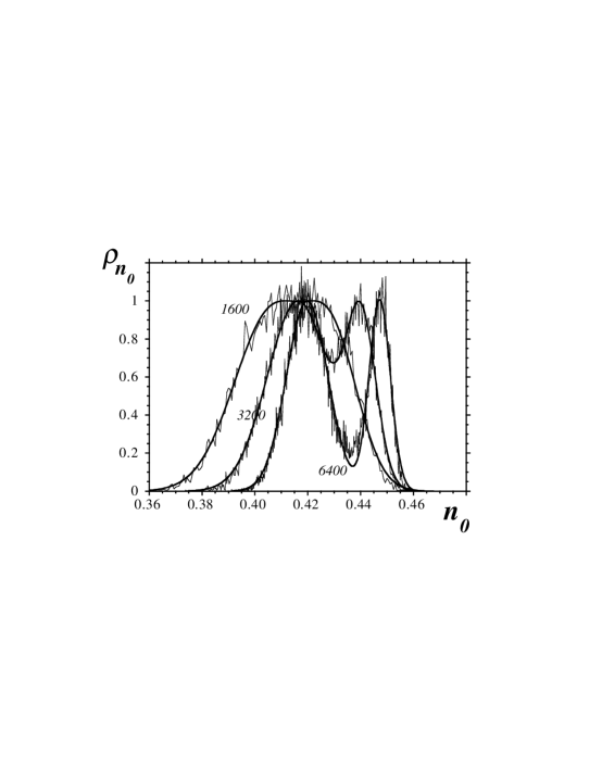
Figure 7: The energy-density distribution $\rho(n_{0})$ for $N_{3}=1600$, 3200 and 64000. The thin lines are the measured distributions, the thick lines are fits to two Gaussian peaks Eq. (8). Each distributions is normalized with the height of the peaks and the values of $\kappa$ chosen so the two peaks are of equal height.

Additional evidence for a phase transition comes from other geometric observables such as the maximal order of a vertex, $q_{0}$. As discussed in the Introduction, the crumpled phase is dominated by triangulations containing few vertexes of very large order, whereas in a branched polymer phase the vertex orders are more or less equally distributed. This is reflected in a sudden drop in the maximal vertex order across the transition; this change leads to divergent peaks in both the fluctuations of $q_{0}$, i.e. the susceptibility $\chi_{q_{0}}=N_{3}\;(\langle q_{0}^{2}\rangle-\langle q_{0}\rangle^{2})$, and its energy derivative ${\rm D}_{q_{0}}=N_{3}\;(\langle q_{0}n_{0}\rangle-\langle q_{0}\rangle\langle n_{0}\rangle)$. In fact, plots of both $\chi_{q_{0}}$ and ${\rm D}_{q_{0}}$ look more or less identical to Figure 6. For all the observables the peak heights diverge, an example of this is shown in Figure 8 for the specific heat. I have estimated the corresponding scaling behavior, fitting the peak values to the form: ${\cal O}_{peak}\sim N_{3}^{\alpha}$; the fitted scaling exponents are shown in Table 1. Compared to $\chi_{q_{0}}$ and ${\rm D}_{q_{0}}$, the fit of the specific heat is rendered considerable more difficult by an additional constant contribution to the scaling behavior. Nevertheless, for the specific heat the peak height scales almost linearly for sufficiently large target volume as is expected for a discontinuous phase transition.

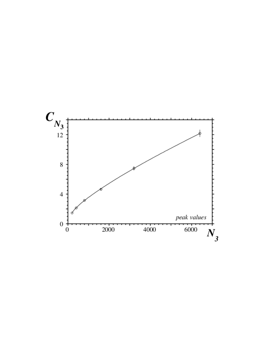
Figure 8: The volume scaling of the peak in the specific heat. The solid line is a fit to the scaling form: $C_{N_{3}}\approx a+bN_{3}^{\alpha}$. The value of the exponent $\alpha$ is shown in Table 1.

To locate the infinite volume critical coupling $\bar{\kappa}_{c}$ I fit the pseudo-critical couplings $\kappa_{c}(N_{3})$, defined by the location of peaks in the different observables, to the expected finite-volume scaling behavior:

$$\kappa_{c}(N_{3})\;=\;\bar{\kappa}_{c}+\frac{const.}{N_{3}^{x}}.$$ (9)

The fitted values of $\bar{\kappa}_{c}$ and the exponent $x$ are shown in Table 1. To asses the finite-size effects I repeated the fits with a different lower cut-off on the included target volume. This did not affect the estimate of $\bar{\kappa}_{c}$ appreciatively; in all cases $\bar{\kappa}_{c}\approx 3.8$. Note however that, in contrast to what has recently been reported in simulations with combinatorial triangulations [6], I observe no indication of the peak locations running to $\bar{\kappa}_{c}=\infty$. For all the observables the pseudo-critical couplings converge nicely. This is shown in Figure 9. A fit to an assumption of non-convergence, $\kappa_{c}(N_{3})=a+b\log N_{3}$, is ruled out by a $\chi^{2}/({\rm d.o.f.})\gtrsim 1000$. For the scaling exponent $x$, I get values $x\approx 1/3$. For a discontinuous phase transition one would naively expect $\delta\kappa_{c}=|\kappa_{c}(N_{3})-\bar{\kappa_{c}}|\sim L^{-d_{H}}$, where $L$ is some appropriate length scale in the system and $d_{H}$ is the (internal) fractal dimension (see e.g. Ref. [14]). This would imply $x=1$ in Eq. (9). However, for a system with a fluctuating internal geometry like simplicial gravity, it is not clear what dimensionality should be associated to the system at a discontinuous phase transition where in one phase the internal fractal dimension is infinite, but two in the other. Hence it is not obvious how to interpret the observed value of the exponent $x$.

Table 1: (A) The volume scaling of the peaks in $C_{N_{3}}$, $\chi_{q_{0}}$ and ${\rm D}_{q_{0}}$, fitted to the form: $a+b\bar{N}_{3}^{\alpha}$, together with the quality of the fits. For $\chi_{q_{0}}$ and ${\rm D}_{q_{0}}$ I use $a=0$. Values are shown for different lower cut-off $N_{3}^{min}$ on the target volume include in the fit. (B) The corresponding values of $\bar{\kappa}_{c}$, determined from fitting the pseudo-critical coupling constants $\kappa_{c}(N_{3})$ to the form Eq. (9), together with the scaling exponent $x$.

$N_{3}^{min}$	$C_{N_{3}}$			$\chi_{q_{0}}$			${\rm D}_{q_{0}}$
(A)
	$\alpha$		$\chi^{2}$	$\alpha$		$\chi^{2}$	$\alpha$		$\chi^{2}$
$200$	0.80(5)		2.5	0.78(2)		3.7	0.66(4)		0.7
$400$	0.80(7)		1.0	0.77(2)		2.8	0.66(5)		0.5
$800$	0.85(12)		0.5	0.76(1)		0.6	0.66(7)		0.3
(B)
	$\bar{\kappa}_{c}$	$x$	$\chi^{2}$	$\bar{\kappa}_{c}$	$x$	$\chi^{2}$	$\bar{\kappa}_{c}$	$x$	$\chi^{2}$
$200$	3.755(22)	0.36(2)	8.5	3.790(19)	0.32(2)	4.8	3.755(22)	0.27(5)	24
$400$	3.741(37)	0.37(3)	7.5	3.829(22)	0.31(2)	2.3	4.10(14)	0.22(5)	12
$800$	3.95(18)	0.27(7)	8.5	3.49(27)	0.26(7)	2	4.07(43)	0.21(9)	11

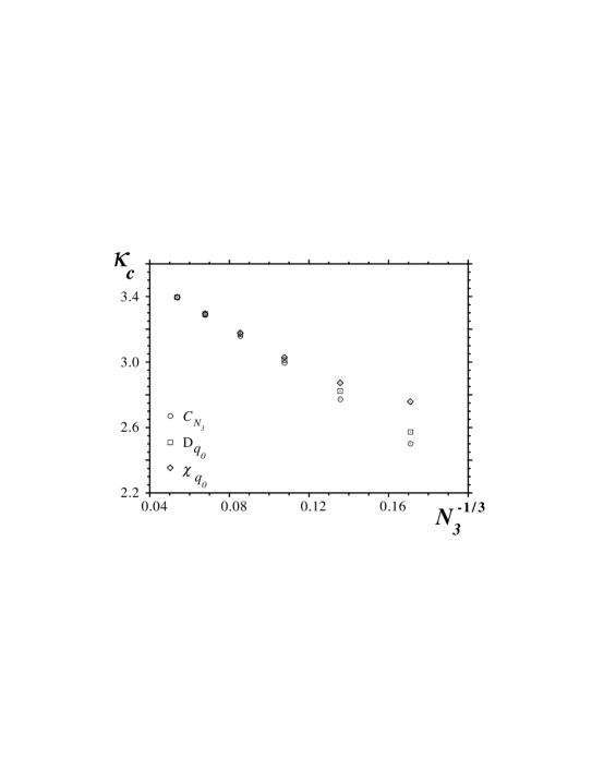
Figure 9: Scaling of the pseudo-critical inverse Newton’s constant $\kappa_{c}(N_{3})$, defined by the location of peaks in $C_{N_{3}}$, $\chi_{q_{0}}$ and ${\rm D}_{q_{0}}$ respectively. The values are plotted versus the volume $N_{3}$ scaled with an exponent $x=1/3$.

4.2 The crumpled phase

As already stated the strong-coupling phase of the model Eq. (2) is a crumpled phase, characterized by few vertexes of very large order. Qualitatively I observe this behavior regardless of the type of triangulations I simulated. Note, however, that there is a priori no reason to expect exactly the same behavior for the two ensembles in this phase; because of the collapsed nature of manifolds it is unlikely that any sensible continuum limit can be taken for $\kappa<\kappa_{c}$. Hence the details of the triangulations — the discretization — may be relevant in the infinite volume limit.

There does indeed appear to be some slight difference in the internal geometry of the ensemble of degenerate triangulations, compared to the combinatorial ensemble, for $\kappa=0$. An example of this is the scaling behavior of the effective critical cosmological constant determined in Section 3. For combinatorial triangulations the exponent of the power-law correction is $\gamma\approx 0.3$, whereas $\gamma\approx 0.5$ for degenerate triangulations. Similar difference is observed in the volume scaling of the order of the most singular vertex. For three-dimensional combinatorial triangulations $q_{0}$ scales sub-linearly with volume: $q_{0}\sim N_{3}^{0.42(2)}$, for degenerate triangulations, on the other hand, the scaling exponent is larger; $q_{0}\sim N_{3}^{0.60(5)}$.

The collapsed nature of this phase is most easily demonstrated by measuring the fractal dimensions $d_{H}$. To estimate $d_{H}$ I measure the two-point correlation function $g_{N_{3}}(r)$, defined as the number of simplexes at a geodesic distance $r$ from a marked simplex. The geodesic distance between two simplexes is defined as the shortest path traversed through the center of simplexes. Assuming that the only relevant length scale in the system is given by $N_{3}^{1/d_{H}}$, general scaling arguments [15] imply that

$$g_{N_{3}}(r)\;\sim\;N_{3}^{1-1/d_{H}}\;F(x),\qquad x\;=\;\frac{r}{N_{3}^{1/d_{H}}}.$$ (10)

The fractal dimension is measured by ”collapsing“ distributions $g_{N_{3}}(r)$, corresponding to different volumes, onto a single scaling curve. I have done this for volume $N_{3}\lesssim 6400$ and for $\kappa=0$; the value of $d_{H}$, determined by minimizing the $\chi^{2}$–value of the collapse, is shown in Table 2. The errors are estimated using jack-knifing. To demonstrate how the estimate of $d_{H}$ depends on the volume, I have done the analysis either including all the volumes, or using pairs of consecutive volumes $N_{3}$ and $2N_{3}$. For $\kappa=0$ the estimate of $d_{H}$ drifts systematically toward larger values as the volume is increased, in addition the fit to the scaling behavior Eq. (10) is very poor; the $\chi^{2}$/(d.o.f.) $>>1$. This is not unexpected, in a crumpled phase the internal fractal dimension is $d_{H}=\infty$, in which case the simplex-simplex correlation function is not expected to scale.

Table 2: The fractal dimension $d_{H}$ for an ensemble of degenerate three-dimensional triangulations, determined by collapsing the simplex-simplex correlation function $g_{N_{3}}(r)$ onto the scaling form Eq. (10). The values shown are for $\kappa=0$ in the crumpled phase, and $\kappa=5$ and 8 in the branched polymer phase. The analysis is done including different target volumes $N_{3}$. Also included is the $\chi^{2}/({\rm d.o.f.})$ value of the collapse.

	$\kappa=0$		$\kappa=5$		$\kappa=8$
{$N_{3}^{min}$—$N_{3}^{max}$}	$d_{H}$	$\chi^{2}$	$d_{H}$	$\chi^{2}$	$d_{H}$	$\chi^{2}$
{200 — 400}	4.05(15)	55	1.85(6)	0.64	1.89(5)	0.55
{400 — 800}	4.66(18)	62	1.92(8)	0.84	1.95(7)	0.55
{800 — 1600}	5.27(14)	50	1.93(8)	0.77	1.93(13)	0.32
{1600 — 3200}	5.68(16)	32	2.00(13)	0.45	1.98(15)	0.58
{3200 — 6400}	6.25(20)	30	1.99(15)	0.45	1.96(12)	0.50
{400 — 6400}	5.20(30)	84	1.94(10)	1.1	1.95(11)	0.6

4.3 The branched polymer phase

Finally I have also investigated the nature of the weak-coupling phase for degenerate triangulations at two values of the coupling constant: $\kappa=5$ and 8. To establish that this is a branched polymer phase I measured both the fractal dimension $d_{H}$ and the string susceptibility exponent $\gamma_{s}$. The estimate of $d_{H}$ is included Table 2. In contrast to the crumpled phase in this phase I get a consistent value $d_{H}\approx 2$, as expected for branched polymers; for both values of $\kappa$ the quality of the scaling is very good, $\chi^{2}/{\rm(d.o.f.)}\lesssim 1$. An example of the scaling is shown in Figure 10 for $\kappa=5$.

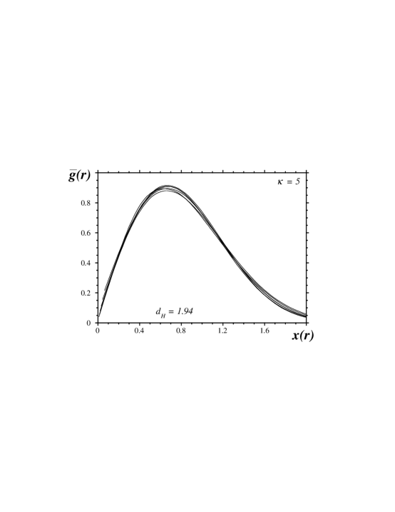
Figure 10: The scaled simplex-simplex correlation function $\bar{g}_{N_{3}}(x)=g_{N_{3}}(x)/N_{3}^{1-1/d_{H}}$ versus the scaling variable $x=r/N^{1/d_{H}}$. This is for degenerate three-dimensional triangulations of size $N_{3}=400$ to 6400 and $\kappa=5$. The measured value of $d_{H}=1.94$ has been used in the scaling.

The string susceptibility exponent $\gamma_{s}$ defines the sub-leading correction to the large-volume behavior of the canonical partition function: $\Omega_{N_{3}}\sim\exp\{\mu_{c}N_{3}\}N_{3}^{\gamma_{s}-3}$. An efficient method for determining $\gamma_{s}$ in quasi-canonical simulations is provided by the size distribution of baby universes. A baby universe is a part of a triangulation connected to the rest via a small “neck”, usually chosen as a minimal neck [16]. For a three-dimensional combinatorial triangulation a minimal neck consists of four triangles glued together along their edges into a closed surface (a tetrahedra). By cutting the triangulation up along this boundary it is divided into two parts; a ”mother“ of size $N_{3}-B$ and a ”baby“ of size $B$. The size distribution of baby universes, $b_{C_{4}}(B)$, is defined as all such partitions averaged over the ensemble. From the asymptotic behavior of the canonical partition function it follows that

$$b_{C_{4}}(B)\;=\;\frac{B\;\Omega_{B}\;(N_{3}-B)\;\Omega_{N_{3}-B}}{\Omega_{N_{3}}}\;\sim\;\left[B(N_{3}-B)\right]^{\gamma_{s}-2}$$ (11)

The distribution $b_{C_{4}}(B)$ can be measured with high accuracy in quasi-canonical simulations and the exponent $\gamma_{s}$ is extracted by a fit to Eq. (11).

The above definition of a baby universe also applies to degenerate triangulations although in this case a minimal neck consist of only two triangles glued together along their three edges (see e.g. Figure 2b). This defines a distribution of baby universes, $b_{D_{2}}(B)$, separated from the rest by two links in the dual graph. It is also possible to define a distribution of baby universes, $b_{D_{4}}(B)$, separated from the rest by four links in the dual graph, analogous to the definition for combinatorial triangulations. I have verified that the two distributions, $b_{D_{2}}(B)$ and $b_{D_{4}}(B)$, lead to the same estimate of $\gamma_{s}$.

I measured the distributions for $\kappa=5$ and on volumes $N_{3}=200$, 400 and 800, and estimated $\gamma_{s}$ by a fit to Eq. (11). This gave the following estimates: $\gamma_{s}=0.47(3)$, 0.48(3) and 0.44(4), for $N_{3}=200$, 400 and 800, respectively. This agrees reasonable with the expected value for branched polymers, $\gamma_{s}=1/2$, especially given the small size of the triangulations used in the estimate.

5 Discussion

I have investigated a model of three-dimensional simplicial gravity defined with an ensemble of degenerate triangulations allowing distinct simplexes sharing the same set of vertexes. The motivation for using degenerate triangulations, instead of the combinatorial ones traditionally used in simplicial gravity for $D>2$, is the experience from two-dimensional simplicial gravity which shows that using less restricted triangulations, i.e. a larger triangulations-space, substantially reduces the finite-size effects in numerical simulations.

As in two dimensions using a different ensemble of triangulations, provided it yields a well defined statistical model, does not seem to change the phase structure of the model; I still observe a crumpled and a branched polymer phase, separated by a discontinuous phase transition. There is, however, evidence of less finite-size effects in the model, especially in the crumpled phase where the critical cosmological constant approaches much faster its infinite volume value. As a consequence, an exponential bound on the number of degenerate triangulations of a given volume is more easily established than for the corresponding ensemble of combinatorial triangulations. This reduction in finite-size effects in the crumpled phase is intuitively clear; with less restrictions on the connectivity of the simplexes the degenerate triangulations crumple more easily. In addition, the discontinuous nature of the phase transition is easily observed on triangulations of relatively modest size.

A natural extension of the work presented in this paper is to add a measure term [17], or alternatively matter fields [18], to the action Eq. (2) and to investigate if the phase structure of the model is modified in the same way as has recently been observed in simulations with combinatorial triangulations in both four [19] and three dimensions [20]. There a new phase — a crinkled phase — appears for a sufficiently large negative coupling to the measure term, or if several matter fields are coupled to the model. If this phase structure does indeed represent some behavior of the continuum it is plausible, based on the expectation of universality, that it should not depend on the details of the discretization and should also be present for degenerate triangulations. Thus corresponding simulations of modified models of three-dimensional simplicial gravity using degenerate triangulations could serve as a confirmation on the observed phase structure. This work is in progress.

Although the result of my numerical investigation of maximally degenerate three-dimensional triangulations indicated that this ensemble does not lead to a well defined statistical model, I do not rule out the possibility that a less restricted ensemble of triangulations, than considered in this paper, could be used. The challenge is to identify an appropriate easing of the restriction which defines a consistent, exponentially bounded, canonical ensemble. With the potential benefits provided by an even larger ensemble than restricted degenerate triangulations this is definitely worth investigating.

Acknowledgments: I would like to thank Piotr Bialas, Sven Bilke and Bengt Petersson for stimulating discussions. This work was supported by the Humboldt Foundation.

References

- [1]
- [2] F. David, Simplicial Quantum Gravity and Random Lattices, (hep-th/9303127), Lectures given at Les Houches Summer School on Gravitation and Quantizations, Session LVII, Les Houches, France, 1992;
- [3] J. Ambjørn, B. Durhuus and T. Jonsson, Quantum Geometry: A statistical field theory approach, (Cambridge University Press, 1997).
-
[4]
J. Ambjørn and S. Varsted,
Phys. Lett. B266 (1991) 285;
Nucl. Phys. B373 (1992) 557;
D.V. Boulatov and A. Krzywicki,
Mod. Phys. Lett. A6 (1991) 3005;
J. Ambjørn, D.V. Boulatov, A. Krzywicki and S. Varsted, Phys. Lett. B276 (1992) 432. - [5] S. Catterall, J. Kogut and R. Renken, Phys. Lett. B342 (1995) 53; Nucl. Phys. B523 (1998) 553.
- [6] T. Hotta, T. Izubuchi and J. Nishimura, Nucl. Phys. 63 (Proc. Suppl) (1998) 63; Multicanonical simulation of 3-d dynamical triangulation model and a new phase structure, (hep-lat/9802021).
-
[7]
H. Hagura, N. Tsuda and T. Yukawa,
Phys. Lett. B418 (1998) 273;
H.S.Egawa, N.Tsuda and T. Yukawa, Common structures in simplicial quantum gravity, (hep-lat/9802010). - [8] E. Brezin, C. Itzykson, G. Parisi and J.B. Zuber, Commun. Math. Phys. 59 (1978) 35.
- [9] J. Ambjørn, G. Thorleifsson and M. Wexler, Nucl. Phys. B439(1995) 187.
-
[10]
M. Bowick, S. Catterall and G. Thorleifsson,
Phys. Lett. B391(1997) 305;
Nucl. Phys. 53 (Proc.Suppl) (1997) 753;
V.A. Kazakov, M. Staudacher and T. Wynter, Nucl. Phys. B471 (1996) 309. -
[11]
N. Godfrey and M. Gross,
Phys. Rev. D43 (1991) R1749;
M. Agishtein and A. Migdal, Mod. Phys. Let. A6 (1991) 1863;
M. Gross and S. Varsted, Nucl. Phys. B378 (1992) 367. - [12] S. Catterall, Comput. Phys. Commun. 87 (1995) 409.
-
[13]
T. Hotta, T. Izubuchi and J. Nishimura,
Prog. Theor. Phys. 94 (1995) 263;
S. Catterall, G. Thorleifsson, J. Kogut and R. Renken, Nucl. Phys. B468 (1996) 263;
P. Bialas, Z. Burda, B. Petersson and J. Tabaczek, Nucl. Phys. B495 (1997) 463;
S. Catterall, J. Kogut and R. Renken, Phys. Lett. B416 (1998) 274. - [14] K. Binder, in The Monte Carlo method in condensed matter physics, ed. K. Binder, 2nd edition, Springe-Verlag 1992.
- [15] S. Catterall, G. Thorleifsson, M. Bowick and V. John, Phys. Lett. B354 (1995) 56; J. Ambjørn, J. Jurkiewicz and Y. Watabiki, Nucl. Phys. B454 (1995) 313.
-
[16]
S. Jain and S.D. Mathur, Phys. Lett. B286 (1992) 239;
J. Ambjørn, S. Jain and G. Thorleifsson, Phys. Lett. B307 (1993) 34;
J. Ambjørn and G. Thorleifsson, Phys. Lett. B323 7(1994) 7. - [17] B. Brugmann and E. Marinari, Phys. Rev. Lett. 70 (1993) 1908.
-
[18]
R.L. Renken, S.M. Catterall and J. Kogut,
Nucl. Phys. B422 (1994) 677;
J. Ambjørn, J. Jurkiewicz, S. Bilke, Z. Burda and B. Petersson, Mod. Phys. Lett. A9 (1994) 2527;
J. Ambjorn, Z. Burda, J. Jurkiewicz and C.F. Kristjansen, Phys. Lett. B297 (1992) 253. - [19] S. Bilke, Z. Burda, A. Krzywicki, B. Petersson, J. Tabaczek and G. Thorleifsson, Phys. Lett. B418 (1998) 266; 4D simplicial quantum gravity: Matter fields and the corresponding effective action, (hep-lat/9804011).
- [20] B. Petersson, O. Prauss, G. Thorleifsson and T. Westheider, in preperation.
- [21]