DESY 98-088

String breaking in SU(2) gauge theory
with scalar matter fields

Francesco Knechtli and Rainer Sommer
DESY

Platanenallee 6, D-15738 Zeuthen

Abstract We investigate the static potential in the confinement phase of the SU(2) Higgs model on the lattice, where this model is expected to have properties similar to QCD. We observe that Wilson loops are inadequate to determine the potential at large distances, where the formation of two color-neutral mesons is expected. Introducing smeared fields and a suitable matrix correlation function, we are able to overcome this difficulty. We observe string breaking at a distance $r_{\rm b}\approx 1.8r_{0}$, where the length scale $r_{0}$ has a value $r_{0}\approx 0.5\,{\rm fm}$ in QCD. The method presented here may lead the way towards a treatment of string breaking in QCD.

DESY 98-088

July 1998

1 Introduction

Since the seminal work by Creutz [?], there have been a number of detailed studies of the static potential in non-Abelian gauge theories. At large distances, there is a linear confinement potential between a source anti-source pair in the fundamental representation of the gauge group. This was clearly established by Monte Carlo calculations of the lattice theories close to the continuum limit, both for gauge groups ${\rm SU(2)}$ [?,?] and ${\rm SU(3)}$ [?,?]. When these gauge theories are coupled to matter fields in the fundamental representation, one does expect that the potential flattens at large distances and asymptotically turns into a Yukawa form. At such distances the potential is better interpreted as the potential between static color-neutral “mesons”, which are bound states of a static color source and the dynamical matter field. So far, this expectation could not be verified by Monte Carlo simulations. In particular, in recent attempts in QCD with two flavors of dynamical quarks this string breaking effect was not visible [?,?,?,?]. The same behavior of the potential is, of course, expected in the non-Abelian Higgs model in the confinement phase. While the potential in the large distance range could not be calculated in early simulations with gauge group ${\rm SU(2)}$, they yielded some qualitative evidence for screening of the potential [?,?]. Similarly, the potential between static adjoint charges is screened by the gauge fields themselves. Numerical evidence for this has been found for gauge group ${\rm SU(2)}$ [?].

In this letter we consider the ${\rm SU(2)}$ Higgs model (in four dimensions) as a first test case and demonstrate that string breaking exists. In order to roughly compare the physical situation in the Higgs model with the one in QCD, we choose a common reference energy scale. One immediately thinks of using the string tension. However, due to the phenomenon of string breaking itself, the string tension does not have a precise meaning (there is no range of $r$ where the potential is linear) and exists only in an approximate sense. It is better to fix the overall scale by $r_{0}$, defined as [?]

$$\left.r^{2}F(r)\right|_{r=r_{0}}=1.65\,,$$ (1)

where $F(r)$ denotes the force derived from the static potential discussed above. The number on the r.h.s. of eq. (1) has been chosen such that $r_{0}$ has a value (estimated from phenomenological potential models describing charm- and bottom-onia) of

$$r_{0}\approx 0.5\,{\rm fm}$$ (2)

in QCD. In the following, all dimensionful quantities are measured in units of $r_{0}$, which is not related to any phenomenological value in the ${\rm SU(2)}$ Higgs model. In QCD with light quarks, the distance $r_{\rm b}$ around which the potential should start flattening off, could be estimated in the quenched approximation [?]:

$$r_{\rm b}\approx 2.7\,r_{0}\,\,\,\mbox{(in QCD)}\,.$$ (3)

2 The Higgs model on the lattice

Working on a four-dimensional hyper-cubic lattice with spacing $a$ we denote by $\Phi(x)$ a complex Higgs field in the fundamental representation of the gauge group SU(2) and $U(x,\mu)\in{\rm SU(2)}$ is the gauge field link connecting $x+a\hat{\mu}$ with $x$. We use the Greek symbols, $\mu,\;\nu$, to denote all directions 0,1,2,3 and Roman symbols such as $k$ to denote the space-like directions 1,2,3. The Euclidean action for the SU(2) Higgs Model is then given as

$$S = \sum_{x}a^{4}\{\sum_{\mu}(\nabla_{\mu}\Phi(x))^{\dagger}\nabla_{\mu}\Phi(x)-m_{0}^{2}\Phi^{\dagger}(x)\Phi(x)+\lambda_{0}[\Phi^{\dagger}(x)\Phi(x)]^{2}\}$$ (4)

$$+\sum_{p}\beta\{1-\hbox{$1\over 2$}\,\hbox{tr}\,U_{p}\}\,,$$

$$U_{p}(x) = U(x,\mu)U(x+a\hat{\mu},\nu)U^{\dagger}(x+a\hat{\nu},\mu)U^{\dagger}(x,\nu)\,,\quad\sum_{p}\,=\,\sum_{x}\sum_{0\leq\mu<\nu\leq 3}\,,$$

where we used the lattice covariant derivative, $\nabla_{\mu}\Phi(x)=\hbox{$1\over a$}\left[U(x,\mu)\Phi(x+a\hat{\mu})-\Phi(x)\right]$. Following conventional notation [?], the bare parameters chosen in the present investigation are given by

$$\beta = 2.2\,,$$

$$\kappa = (1-2\lambda)/(8-a^{2}m_{0}^{2})\,=\,0.274\,,$$ (5)

$$\lambda = \kappa^{2}\lambda_{0}\,=\,0.5\,.$$

This point in parameter space is in the confinement phase, fairly close to the phase transition, where the model has properties similar to QCD [?,?]. The lattice resolution is of roughly the same size as the one used in the QCD-studies quoted above: from the potential calculation detailed in the following section, we obtained

$$r_{0}/a = 2.83\pm 0.03\,.$$ (6)

While one cannot expect a very precise result for the detailed form of the potential with such a resolution, it is expected that qualitative features are correctly described.

The string breaking distance $r_{\rm b}$ depends directly on the mass of the static mesons which in turn is sensitive to the bare mass, $m_{0}$, of the scalar fields. For our chosen value of $m_{0}$, the string breaking distance, $r_{\rm b}$, is somewhat smaller than the estimate quoted above for quenched QCD. Nevertheless, the physical situation is quite similar. We note in passing that the self-coupling of the Higgs field, $\lambda_{0}$, appears to have little influence on the physics of the Higgs model in the confinement phase [?].

3 Calculation of the potential at all distances

We now introduce a method, which – as we will demonstrate in the following section – allows to compute the potential, $V(r)$, at all relevant distances in the theory with matter fields. Before explaining the details, we would like to mention the basic point, which has first been noted by C. Michael [?]. Mathematically, the method is based on the existence of the transfer matrix [?] and the fact that it can be employed also when external static sources are present (see e.g. [?]). In the path integral, a static source at position $\bf x$, together with an anti-source at position ${\bf x}_{r}\,=\,{\bf x}+r\hat{k}$, are represented by straight time-like Wilson lines fixed at these space-positions. These Wilson lines have to be present in any (matrix) correlation function from which one wants to compute the potential energy of these charges. The space-like parts of the correlation functions, which are again Wilson lines when one considers standard Wilson loops, do not determine which states appear in the spectral representation of the correlation functions. They do, however, influence the weight with which different states contribute. For these space-like parts, we therefore use both Wilson lines which will have large overlap with string-like states and Higgs fields with a dominant overlap with meson-type states. Combining them in a matrix correlation function, the correct linear combination which gives the ground state in the presence of charges can be found systematically by the variational method described below.

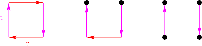
Figure 1: The correlation functions used to determine the static potential, from left to right: $C_{\rm WW}$, $C_{\rm WM}$ and $C_{\rm MM}$. The lines represent the Wilson lines, the filled circles the Higgs field.

Let us now give precise definitions of the correlation functions, which are illustrated in Fig. 1. For small values of $r$ or in the pure gauge theory, the static potential can be efficiently computed by means of Wilson loops,

$$C_{\rm WW}(r,t) = \langle\,\hbox{tr}\,[W(x,x_{r})\,W(x_{r},x_{r}+t\hat{0})\,W^{\dagger}(x+t\hat{0},x_{r}+t\hat{0})\,W^{\dagger}(x,x+t\hat{0})]\rangle$$ (7)

$${}_{\mbox{$\stackrel{{\scriptstyle\displaystyle\sim}}{{\scriptstyle t\rightarrow\infty}}$}} {\rm const.}\times{\rm e}^{-V(r)t}\,,$$

where $x_{r}\,=\,x+r\hat{k}$ and $W(x,y)$ denotes the product of gauge links along the straight line connecting $y$ with $x$. In addition, one may compute the mass, $\mu$, of a static meson from the correlation function

$$C_{\rm M}(t)=\langle\Phi^{\dagger}(x)\,W(x,x+t\hat{0})\,\Phi(x+t\hat{0})\rangle\;_{\mbox{$\stackrel{{\scriptstyle\displaystyle\sim}}{{\scriptstyle t\rightarrow\infty}}$}}\;{\rm const.}\times{\rm e}^{-\mu t}\,.$$ (8)

Consequently, we expect that for distances significantly larger than $r_{\rm b}$, where the relevant states correspond to weakly interacting mesons, the potential is close to the value $\lim_{r\to\infty}V(r)=2\mu$ and can be extracted from the correlation function

$$C_{\rm MM}(r,t)=\langle\Phi^{\dagger}(x+t\hat{0})W^{\dagger}(x,x+t\hat{0})\Phi(x)\,\,\,\Phi^{\dagger}(x_{r})W(x_{r},x_{r}+t\hat{0})\Phi(x_{r}+t\hat{0})\rangle\,.$$ (9)

In order to investigate all (and in particular the intermediate) distances, we introduce a (real) symmetric matrix correlation function $C_{ij}(r,t)$, $i,j\in\{\rm W,M\}$ with

$$C_{\rm WM}(r,t)=\langle\Phi^{\dagger}(x+t\hat{0})\,W^{\dagger}(x,x+t\hat{0})\,W(x,x_{r})\,W(x_{r},x_{r}+t\hat{0})\,\Phi(x_{r}+t\hat{0})\rangle\,.$$ (10)

For fixed $r$, $V(r)$ is extracted from the matrix correlation in the following way [?]. One first solves the generalized eigenvalue problem,

$$C(t)v_{\alpha}(t,t_{0}) = \lambda_{\alpha}(t,t_{0})C(t_{0})v_{\alpha}(t,t_{0})\quad\lambda_{\alpha}>\lambda_{\alpha+1}\,.$$ (11)

According to a general lemma proven in [?], the ground state energy $V(r)\equiv V_{0}(r)$ and the excited states energies $V_{1}(r),\;...$ are then given by

$$aV_{\alpha}(r) = \ln(\lambda_{\alpha}(t-a,t_{0})/\lambda_{\alpha}(t,t_{0}))+{\rm O}\left({\rm e}^{-(V_{N}(r)-V_{\alpha}(r))t}\right)\,.$$ (12)

Here, $N$ is the rank of the matrix $C$. So far we have $N=2$ and for this small value of $N$ the method would require large values of $t$ for the correction terms in eq. (12) to be negligible.

To improve on this, we introduce smeared space-like links [?], setting the smearing strength $\epsilon$ of [?] to the numerical value $\epsilon\,=\,1/4$. For the Higgs field we employ a smearing operator, $\mathcal{S}$, defined as

$$\mathcal{S}\Phi(x) = \mathcal{P}\{\mathcal{P}\Phi(x)+\mathcal{P}\sum_{|x-y|=\sqrt{2}a\atop x_{0}=y_{0}}\overline{U}(x,y)\Phi(y)+\mathcal{P}\sum_{|x-y|=\sqrt{3}a\atop x_{0}=y_{0}}\overline{U}(x,y)\Phi(y)\}\,,$$ (13)

where $\mathcal{P}\Phi=\Phi/\sqrt{\Phi^{\dagger}\Phi}$ and $\overline{U}(x,y)$ represents the average over the shortest link connections between $y$ and $x$.

For different smearing levels $m=1,...,N_{\Phi}$ we evaluate the correlation functions introduced above with $\Phi(x)$ replaced by $\Phi^{(m)}(x)=\mathcal{S}^{m}\Phi(x)$ and similarly with $m=0,1,...,N_{\rm U}$ smearing iterations of the space-like gauge fields, where $m=0$ corresponds to the unsmeared gauge links. This defines a correlation matrix $C$ with rank $N=N_{\Phi}+N_{\rm U}+1$.

Figure 2: Ground state energy of a static meson.

4 String breaking

We now turn to discuss our numerical results obtained on a $20^{4}$ lattice with periodic boundary conditions. The Higgs model can be simulated efficiently with a hybrid over–relaxation algorithm. In particular, we implemented the over–relaxation for the Higgs field as described in [?]. After a rough tuning of the mixture of the various parts of the updating we found that autocorrelations are no problem in our simulations. Errors were computed by a jacknife analysis.

We computed all correlation functions up to $r_{\rm max}=t_{\rm max}=8a\sim 3\,r_{0}$ on 2000 field configurations. We set $N_{\Phi}=4$ and $N_{\rm U}=2$. The variance of the correlation functions was reduced in different ways. We used translational invariance to average over the base point denoted by $x$ in eqs.(7-10) and cubic symmetry to average over the different orientations $\hat{k}$. Finally, statistical errors were further reduced by replacing – wherever possible – the time-like links by the 1-link integral [?], which can be evaluated analytically for the gauge group SU(2).

Figure 3: Comparison of the static potential computed from eq. (12) using the full correlation matrix and the sub-block with the (smeared) Wilson loops. Two representative values of $r$ are shown.

Figure 4: The static potential in units of $r_{0}$. The asymptotic value $2\mu$ has been subtracted to obtain a quantity free of self energy contributions which diverge like $1\over a$.

The first quantity one wants to know is the mass of the static mesons, since this fixes the asymptotic value of the potential. It is best computed from the correlation $C_{\rm M}$ extended to a $N_{\Phi}\times N_{\Phi}$ correlation matrix by considering the smeared $\Phi$ fields. As for all other energy levels discussed below, the mass is computed from the eigenvalues of the generalized eigenvalue problem described above, setting $t_{0}=0$. In Fig. 2 the convergence for large $t$ is exemplified. One observes that the ground state energy can be extracted with confidence and with very good statistical precision, $a\mu\,=\,0.698\pm 0.002$ (read off at $t=7a$ which agrees fully with $t=6a$). From the correlation function without smearing a determination of $\mu$ was not possible.

At all distances, the potential $V(r)$ was then computed using the full $7\times 7$ correlation matrix. The convergence of eq. (12) is shown in Fig. 3 (circles). In earlier calculations in QCD, string breaking was searched for in (smeared) Wilson loops. We studied whether one can succeed in this way by restricting the correlation matrix to the corresponding $(N_{\rm U}+1)\times(N_{\rm U}+1)$ sub-block. The resulting potential estimates (triangles in Fig. 3) are very good at short distances but have large correction terms at long distances. Without a very careful analysis one might extract a potential which is too high at large distances, when one uses Wilson loops alone. This might explain why string breaking has not been seen in QCD, yet. In contrast, from our full correlation matrix we can extract safe estimates for $V(r)$ using eq. (12) for $t\approx 6a$.

We then followed the steps described in [?] to determine $r_{0}$ and computed the potential in units of $r_{0}$. Considering in particular the combination $V(r)-2\mu$, one has a quantity free of divergent self energy contributions. It is shown in Fig. 4. The expected string breaking is clearly observed for distances $r>r_{\rm b}\approx 1.8\,r_{0}$. Around $r\approx r_{\rm b}$, the potential changes rapidly from an almost linear rise to an almost constant behavior. To resolve this transition region using a smaller lattice spacing is an interesting challenge to be addressed in the future.

Overlaps of variationally determined wave functions $v_{0}$ are a certain measure for the efficiency of a basis of operators used to construct the correlation functions. To give a precise definition of the overlap, we define the projected correlation function

$$\Omega(t)\;=\;v_{0}^{\rm T}C(t)v_{0}\;=\;\sum_{n}\omega_{n}{\rm e}^{-V_{n}(r)t}\,,\;\mbox{with normalization}\;\Omega(0)=1\,.$$ (14)

Here, $n$ labels the states in the sector of the Hilbert space with 2 static charges. The form given above follows directly in the transfer matrix formalism [?]. The positive coefficients $\omega_{n}$ may be interpreted as the overlap of the true eigenstates of the Hamiltonian with the approximate ground state characterized by $v_{0}$. “The overlap ” is an abbreviation commonly used to denote the ground state overlap, $\omega_{0}$.

Figure 5: Ground state overlaps, once from the full correlation and once from the Wilson loops alone.

We determine $\omega_{0}$ straightforwardly from the correlation function $\Omega(t)$ at large $t$. As shown by the circles in Fig. 5 our operator basis is big (and good) enough such that $\omega_{0}$ exceeds about 60% for all distances. It is now interesting to consider also the overlap for the Wilson loops alone, i.e. we again restrict the correlation matrix to the $(N_{\rm U}+1)\times(N_{\rm U}+1)$ sub-block. Let us denote the corresponding projected correlation function by $\Omega_{\rm W}$ and the overlap by $\omega_{0}^{\rm W}$. The computation of $\omega_{0}^{\rm W}$ is more difficult, because it turns out to be very small at large $r$. Nevertheless, the expression

$$\omega_{0}^{\rm W} {}_{\mbox{$\stackrel{{\scriptstyle\displaystyle\sim}}{{\scriptstyle t\rightarrow\infty}}$}} \omega_{0}{\Omega_{\rm W}(t)\over\Omega(t)}$$ (15)

converges reasonably fast and $\omega_{0}^{\rm W}$ can be estimated from the r.h.s. for $t\approx 6a$. The results plotted in Fig. 5 (triangles) show that Wilson loops alone have an overlap which drops at intermediate distances and are clearly inadequate to extract the ground state at large $r$. Instead, the full matrix correlation function has to be considered if one wants to compute $V(r)$ at all distances.

5 Outlook

We have introduced a method to compute the static potential at all relevant distances in gauge theories with scalar matter fields. We demonstrated that it can be applied successfully in the SU(2) Higgs model with parameters chosen to resemble the situation in QCD. There is little doubt that it can be applied for different values of parameters in the Higgs model, at least as long as $r_{\rm b}/a$ is not too large. It is then interesting to follow a line of constant physics towards smaller lattice spacings in order to check for cutoff effects and to be able to resolve the interesting transition region in the potential. Furthermore, one might be interested in increasing the mass of the Higgs field in order to reach a situation with a larger value of $r_{\rm b}/r_{0}$ which presumably is even closer to the physics situation in QCD.

From the matrix correlation function one can also determine excited state energies. We have done this successfully for the single meson states but a precise determination of the excited potential at all distances needs more statistics. One expects that the transition region of the potential can be described phenomenologically by a level crossing (as function of $r$) of the “two meson state” and the “string state” [?]. We are planning to investigate this in more detail. So far, we can only say that for $r\approx r_{\rm b}$ the two levels $V_{1}(r)$ and $V(r)$ are close.

Of course, it is of considerable interest to apply this method to QCD with dynamical fermions. It is difficult to predict how well this can be done. Finding good smearing operators should not be a problem. However, the correlation functions will involve the quark fields and one cannot easily take advantage of translational invariance to reduce the statistical errors as was done here. Thus, larger statistical uncertainties are expected. On the other hand, in QCD the quark fields are integrated out analytically, which usually results in correlation functions with relatively small statistical errors. Also new methods [?] should be tried and the final statistical errors can only be determined by explicit computations. In any case, the only possible difficulty is expected to be one of statistical accuracy. The proper correlation functions can be constructed along the lines of ref. [?] and of Sect. 3.

The day of completion of this manuscript, a study of string breaking in the three-dimensional SU(2) Higgs model appeared [?]. Both the method applied and the conclusions are very similar to what we find in four dimensions.

Acknowledgement. We thank Jochen Heitger for helpful discussions. Our simulations were performed on the SP2 of DESY at Zeuthen. We thank the staff of the DESY computer center for their support.

References

- [1] M. Creutz, Phys. Rev. D21 (1980) 2308.
- [2] UKQCD, S.P. Booth et al., Nucl. Phys. B394 (1993) 509, hep-lat/9209007.
- [3] R. Sommer, Nucl. Phys. B411 (1994) 839, hep-lat/9310022.
- [4] G.S. Bali and K. Schilling, Phys. Rev. D46 (1992) 2636.
- [5] UKQCD, S.P. Booth et al., Phys. Lett. B294 (1992) 385, hep-lat/9209008.
- [6] SESAM, U. Glässner et al., Phys. Lett. B383 (1996) 98, hep-lat/9604014.
- [7] S. Güsken, Nucl. Phys. Proc. Suppl. 63 (1998) 16, hep-lat/9710075.
- [8] CP-PACS, S. Aoki et al., Nucl. Phys. Proc. Suppl. 63 (1998) 221, hep-lat/9710059.
- [9] UKQCD, M. Talevi, Nucl. Phys. Proc. Suppl. 63 (1998) 227, hep-lat/9709151.
- [10] H.G. Evertz et al., Phys. Lett. 175B (1986) 335.
- [11] W. Bock et al., Z. Phys. C45 (1990) 597.
- [12] C. Michael, Nucl. Phys. B (Proc. Suppl.) 26 (1992) 417.
- [13] R. Sommer, Phys. Rept. 275 (1996) 1, hep-lat/9401037.
- [14] I. Montvay, Nucl. Phys. B269 (1986) 170.
- [15] M. Lüscher, Commun. math. Phys. 54 (1977) 283.
- [16] C. Borgs and E. Seiler, Commun. Math. Phys. 91 (1983) 329.
- [17] M. Lüscher and U. Wolff, Nucl. Phys. B339 (1990) 222.
- [18] APE, M. Albanese et al., Phys. Lett. 192B (1987) 163.
- [19] B. Bunk, Nucl. Phys. B (Proc. Suppl.) 42 (1995) 566.
- [20] G. Parisi, R. Petronzio and F. Rapuano, Phys. Lett. 128B (1983) 418.
- [21] I.T. Drummond, (1998), hep-lat/9805012.
- [22] UKQCD, C. Michael and J. Peisa, (1998), hep-lat/9802015.
- [23] O. Philipsen and H. Wittig, (1998), hep-lat/9807020.