Liverpool LTH 427
Edinburgh 98/12
Tuning Actions and Observables in Lattice QCD
Abstract
We propose a strategy for conducting lattice QCD simulations at fixed volume but variable quark mass so as to investigate the physical effects of dynamical fermions. We present details of techniques which enable this to be carried out effectively, namely the tuning in bare parameter space and efficient stochastic estimation of the fermion determinant. Preliminary results and tests of the method are presented. We discuss further possible applications of these techniques.
12.38.Gc, 11.15.Ha, 02.70.Lq
I Introduction
First results from full simulations of lattice QCD have confirmed the magnitude of the computational task ahead and have shown only glimpses of physics beyond the quenched approximation. A recent survey of results can be found in [1].
Preliminary results by the UKQCD collaboration [2, 3] using an improved action have shown a surprisingly strong dependence of the effective lattice volume on the bare quark mass. This complicates chiral extrapolations of simulation measurements and obscures comparisons with quenched calculations. With this in mind, we investigate how one might control the effective lattice volume by tuning the bare action parameters while the effects of decreasing quark mass are studied.
Before proceeding, we should clarify what we mean by ‘effective lattice volume’. For definiteness, consider the Wilson discretisation of QCD giving a lattice action dependent on two bare parameters and defined in the usual way. In the quenched approximation, we have become used to thinking of as uniquely controlling the lattice spacing . At fixed , one makes lattice measurements of the rho mass or the Sommer scale , defined by [4]
which is conceptually simpler for the present discussion since, in this case, there is no need to consider extrapolation in the (valence) quark mass. One then matches the lattice value of to its physical value ( fm as extracted from heavy quark spectroscopy [4]) to obtain the lattice spacing at that value of . This mapping between and physical lattice spacing is model dependent in that it is unique to the quenched approximation. The continuum limit is not accessible directly since the lattice volume vanishes. One must remain at lattice spacing small enough that discretisation errors are small but not so small that finite volume effects are significant.
There are two ways of extending these ideas in the presence of dynamical fermions controlled by the bare mass parameter .
-
1.
The conventional procedure is to construct a similar mapping between and lattice spacing where the matching is made using the lattice value of extrapolated in (sea quark mass) to the chiral limit. This yields a unique, but regularisation-dependent, mapping . Comparisons with the continuum limit are made as in the quenched case.
-
2.
Alternatively, one may consider matching the lattice value of at finite values of . Here, the picture is that the simulation is being done with sea quarks of non-infinite mass. Each value of the bare quark mass (or ) then corresponds to a different approximation to continuum QCD with light dynamical quarks, in much the same way as does quenched QCD (infinite ). Matching in this case results in a mapping . Clearly, this is also regularisation-dependent.
The term ‘effective lattice volume’ refers to this second definition of lattice spacing. Our proposal, then, is to conduct simulations in which one attempts to hold the effective lattice spacing fixed. In this way one is better able to keep the physics constant, control lattice artifacts and finite volume effects while studying the effects of light dynamical quarks. In contrast, when adopting the first strategy, the significance of lattice artifacts and finite volume effects changes as the chiral extrapolation is made.
In order to carry out this programme one requires a practical way of identifying curves in the plane of constant lattice spacing
| (1) |
Consider , the lattice measurement of observable with dimension , so that
| (2) |
Then, in the scaling region and to leading order, curves of constant yield estimates of these curves of constant lattice spacing. In this way, one can track changes in required to compensate for changes in . As a simple example, one can identify the shift involved in comparisons of quenched and dynamical simulations. In practice, there will be residual dependence on the choice of . We would expect to be a ‘good’ choice for exposing sea quark dependence whereas would not, due to the strong dependence on valence quark mass and the effects of chiral symmetry constraints.
In the rest of the paper, we show how the operator and action matching technology introduced in [5] can be used to identify such curves. We demonstrate efficient algorithms for achieving it and present some numerical tests. In section II we summarise the relevant matching formalism required and how it may be used. In section III we describe an efficient algorithm for making stochastic estimates of the fermion determinant [6, 7]. Results of numerical tests are presented in the next section. This is followed by a discussion of additional applications of these techniques, including parallel tempering simulations with dynamical fermions. Conclusions and outlook are contained in the final section.
II Curves of constant physics
We first review the matching formalism introduced in [5]. Consider actions and describing two lattice gauge theories with the same gauge configuration space so that
| (3) |
For example, might be the quenched Wilson action and the -improved action for 2-flavour QCD [9]. In the present application, we will consider and to be the same improved fermion action but at different points in the plane. Here, is some lattice observable. Expectation values with respect to the two actions can be related via a cumulant expansion whose leading behaviour implies[5]
| (4) | |||
| (5) |
In general, an action is a function of several parameters. For example, the Wilson action depends on the bare parameters and . In [5] we considered matching action parameters in one of three distinct ways
-
M1:
match a given set of operators. i.e. require
-
M2:
minimise the ‘distance’ between the actions, i.e. ;
-
M3:
maximise the acceptance in an exact algorithm for constructed via accept/reject applied to configurations generated with action .
It was shown that, to lowest order, tuning prescriptions M2 and M3 coincide. In fact, if the operators contribute to the action with weights which are considered as tuning parameters, then prescription M1 also coincides to lowest order. The prescriptions differ in a calculable way at next order. Details are in [5].
In the present application we take
| (6) |
and seek to explore the bare parameter dependence of the lattice theory using configurations generated at a series of reference points in parameter space.
Here, is the effective action corresponding to lattice QCD with the fermions integrated out. i. e.
| (7) |
where is the usual Wilson plaquette action
| (8) |
and
| (9) |
The fermion matrix for the non-perturbative improved theory is a function of both and . This is because the parameter [9] is a function of [10]. Since the improvement scheme fixes , one must not treat as an independently tunable parameter. However, as we shall see, the fact that the operator is a function of as well as introduces some practical complications.
According to eqn. 4, one requires measurements of
| (10) |
in order to carry out parameter tuning. We discuss efficient algorithms for this in section III.
For now, consider matching lattice observable at two neighbouring points in the plane:
| (11) |
According to prescription M1 above and (4) we require, to first order in small quantities,
| (12) |
From this we can deduce that the constant curve is given by
| (13) |
where
| (14) |
Equation (13) amounts to a non-linear differential equation since the right hand side involves (via the parameter). Linearising and taking the limit yields for the constant curve,
| (15) |
The quantity
is well determined [10] and so the determination of constant curves reduces to measuring correlations of the form
| (16) |
The details of this will be described in section IV.
As pointed out in the Introduction, the details of these curves will depend on the choice of . For sensible choices and reasonably physical values of the parameters, one would hope that the corresponding curves of constant , say, would agree rather closely, locally at least. For demonstration purposes, we will consider in section IV several simple choices for :
-
, the average plaquette, proportional to .
-
, various Wilson loops.
-
, the complete effective action itself.
-
Correlation matrices for measuring the static potential and .
-
Hadron correlators.
The first of these, , may be readily measured with high accuracy and so is excellent for testing the basic technology. However, it is not expected to shed much light on lattice spacing. The last two are computationally more demanding but more relevant to the project at hand, identifying curves of fixed physical volume.
One might expect that matching the full action () would be more physically relevant than matching the plaquette piece of the action. From (15) we see that this curve is determined by correlations of the form
| (17) |
in addition to those of (16). As we shall see in section IV, it is more difficult to obtain unbiased estimators for these.
Now consider matching scheme M2 where ‘distances’ in the action space are minimised. One can think of this as defining ‘geodesics’ in the plane with respect to the metric implied by (3) i.e.
The corresponding affine connection would be
Simple minimisation yields, to first order,
| (18) |
In section V we show that these curves are directly relevant to simulations of full QCD using parallel tempering. Again, we note that these curves involve operator correlations which are more complex to estimate.
Finally in this section, we observe that some of the above formalism simplifies considerably in the case of the unimproved Wilson action () since then, for example,
| (19) |
III Stochastic estimator of the fermion determinant
We require an unbiased estimator for where is a hermitian positive-definite matrix. We will also require estimators for , and . Bai, Fahey and Golub [6] have recently proposed estimators, with bounds, for quantities of the form
| (20) |
where is some matrix function. In our application is the logarithm and, for convenience of notation, we set
| (21) |
Taking , some normalised noise vector (e.g. or Gaussian), we can obtain a stochastic estimate of via
| (22) |
The corresponding variance of this estimator is
| (23) |
for complex Gaussian noise, and something less than this for noise ( on each of the complex component). In the case of Gaussian noise, we also obtain rather directly an efficient unbiased estimator for ,
| (24) |
where is an unbiased estimator for ,
| (25) |
In the case of noise, the corresponding estimator is not readily accessible via the techniques described below, so we restrict the discussion to complex Gaussian noise.
In a companion paper [11], we give fuller details of methods for evaluating the quantities , and so on. In practice, we make no use of the bounds presented in [6]. Instead we use large enough Lanczos systems so that the numerical convergence renders the bounds irrelevant. The efficiency of the method results from an elegant relationship between the nodes and weights required for a -point Gaussian quadrature and the eigenvalues and eigenvectors (so-called Ritz pairs) of a Lanczos matrix of dimension [6]. In the companion paper [11], we show that this relationship, and resulting accuracy remain good even when orthogonality is lost. This is an important point for our application. If the Lanczos system is large enough to avoid truncation errors, one is well into the regime where orthogonality is lost in standard numerical Lanczos methods. In the present paper we merely summarise the formulae required to obtain the present set of results. Preliminary results using these techniques were presented in [7].
The actual estimator which we use for is
| (26) |
where
| (27) |
Here are the eigenvalues of the -dimensional tridiagonal Lanczos matrix formed using as a starting vector. The weights are related to the corresponding eigenvectors [6]. In fact, is just the first component of the th eigenvalue of the tridiagonal matrix.
The estimator , for , is obtained from (26) and (27) using rather than . For (see (24)), we define
| (28) |
It is straightforward to show that, with the above definitions
| (29) |
and
| (30) |
The above Lanczos-based methods for evaluating are significantly more efficient than Chebychev-based methods used previously [8, 5]. For a given level of accuracy in the present applications, they are between 3 and 5 times more economical in the number of matrix multiplications required. Typically we achieve six figure convergence of the quadrature with 70 Lanczos steps on a matrix with a condition number () of order or .
Our goal was to achieve variance with respect to (see (23)) which was one order of magnitude less than that with respect to the physical (gauge) distribution. We found that was a suitably conservative number of noise vectors to use.
For estimating , we note that
| (31) |
Thus we can achieve variance
| (32) |
if we use
| (33) |
provided we have employed the same set of noise vectors. This is simple to arrange.
In fact, one could use stochastic estimators of the form (20) to estimate directly
| (34) |
An estimator for is obtained by setting
| (35) |
where is a suitable (e.g. Gaussian) noise vector. Then
| (36) |
is an unbiased estimator of as required. For this unsymmetric case (), two Lanczos systems must be used and a subtraction performed [6]. For the present analysis we have used the symmetric formalism as described above. Further analysis and discussion of these and related stochastic estimators is presented in [11].
In the next section we report results of some tests of the matching procedures using the above algorithms.
IV Numerical tests of matching
A Work estimates
Having generated an ensemble of decorrelated configurations, one can consider estimating the numerical derivatives required for matching (see (15)) in one of two ways:
-
1.
conduct two further simulations at neighbouring points in parameter space and make (uncorrelated) measurements of on each of these
-
2.
apply the stochastic trace log techniques of the previous section to the existing ensemble.
One can estimate the relative amount of work involved in these two approaches. Suppose we seek to achieve an absolute error of on a measurement of by each method and that the variances of and of are and respectively. The ratio of work required for the two approaches is then
| (37) |
where is the work done in a stochastic estimate of trace log on one configuration, is the number of trace logs required (either 2 or 3) and is the work done in generating one decorrelated configuration by Hybrid Monte Carlo (HMC). In turn, we estimate
| (38) |
where the various parameters are associated with HMC simulation and the stochastic estimation of the determinant. These are defined in Table I which also shows typical values from the analysis presented below. With the numbers shown, the ratio is about . In Table II we show sample values of the variances and taken from the present study. Putting all this together we estimate
| (39) |
Although the variance of can be quite large on large lattices, it is proportional to , or whatever the relevant difference parameter is. It is therefore possible, in principle, to obtain acceptable accuracy for the relevant derivative by method (2) with significantly less work. The above example suggests this is less than of that required to obtain comparable accuracy by making additional simulations. One can easily refine the above treatment to take account of the work involved in equilibration. Of course, this makes method (2) seem even more attractive.
B Fixed plaquette curve
First, we present results from matching the average plaquette . This provides a check on some basic features of the procedures: the first order truncation of the cumulant expansion (4) and the Lanczos-based noisy estimator algorithm (26). The initial reference point in the plane was taken as
| (40) |
where a sequence of well-equilibrated configurations had been generated by hybrid Monte Carlo on a lattice with the non-perturbatively improved action for 2 flavours [3]. At , the relevant improvement coefficient is [10]. It is estimated from preliminary spectroscopy measurements on larger lattices that is around at this and . The values of considered in this analysis are typical of those being used in production simulations. Plaquette measurements from all trajectories within this data sample showed autocorrelation times less than 20 trajectories. Longer runs showed an autocorrelation time for the plaquette of roughly double this. Bootstrap with binning was used to estimate the errors on all quantities.
Using the algorithm and choices described in section III, we made stochastic estimates of on a sequence of 40 configurations separated by 20 trajectories. In order to make use of (13) and (15) this must be done using a minimum of parameter sets:
| (41) |
Recall that for the unimproved Wilson action, there is no need to account for the additional dependence in which enters via .
Having selected a change in bare quark mass (for example ), we then use (15) with to estimate . This yields a first estimate of the change required to maintain a fixed value of . One can then use (13) to verify this estimate of by making further stochastic estimates of at the final parameter set . In all cases studied, this last verification step has been well satisfied and so one can in fact identify the matching curve directly from the two partial derivatives as proposed in the previous section. Results are shown in Table III.
We have then generated further dynamical fermion configurations at the matched point
| (42) |
and accumulated a similar ensemble of configurations for subsequent measurement. The corresponding value of is . The plaquette measurements were made using relatively high statistics yielding the statistical errors shown. In order to make a proper comparison, one should fold into the error on at that due to the uncertainty in (). This would feed through to an additional uncertainty in of . Thus the matching test is very well satisfied for the plaquette.
The matching prediction done in reverse, back from to , is also seen to be well satisfied. From Table III we see that is expected to match with in good agreement with from where the matching estimates were originally made. Also in Table III, we show the estimated shift corresponding to a further change of in . Steps of this kind allow one to set up a grid of points from which which one can then deduce the fixed plaquette curve in the plane.
For the sake of completeness, we also show in Table III the estimated shift required to match with quenched measurements of (i. e. at infinite ). Independent gauge simulations at show a good match of when one takes into account the additional uncertainty in of around which would feed through from the error of on estimating . Of course, for such large shifts the first order approximation may not be sufficiently accurate. We have calculated the second order approximation to [5] for this quantity (+0.52(10)) but the statistical error is such that one cannot reliably discriminate it from the first order result (+0.41(3)) with the present level of statistics.
A further plaquette matching test is given in Table III. In this example, the reference point for the ‘constant’ plaquette curve was . Again, direct simulation showed that the matching was accurate and self-consistent. The matched points on this curve (), have been used to conduct tests of parallel tempering as described in section V.
C Full action matching
We have noted in section II that some of the correlations required to identify curves of constant action (18) are not directly calculable by the techniques of section III. Those of the form
| (43) |
require some care when setting up unbiased estimators. In particular,
| (44) |
is not unbiased. For an unbiased estimator, one requires something like that used for , i. e. . Unfortunately it is not so easy to evaluate the analogue of (25) via the above Lanczos methods. However, provided the variance of with respect to noise (23) is indeed small compared to that with respect to gauge fluctuations, the estimator (44) provides a useful approximation. Using this approximation, we have measured the shift corresponding to a shift at fixed action to compare with that at fixed plaquette. For the first test shown in Table III, we find (statistical error only) consistent with the value found for the fixed plaquette curve. In each case studied, we have found such consistency.
We conclude that the fixed action and fixed plaquette curves are not significantly different at this order.
D Gauge invariant loops
We are especially interested in matching those observables which are more sensitive to long range physics. We have repeated the above plaquette matching analysis using a variety of Wilson loops. The 16 loops used consist of 4 basic shapes realised in 4 different ‘magnifications’ (, , and ). The 4 basic shapes used were those specified in terms of link steps by the operations shown in Table IV and rotations thereof.
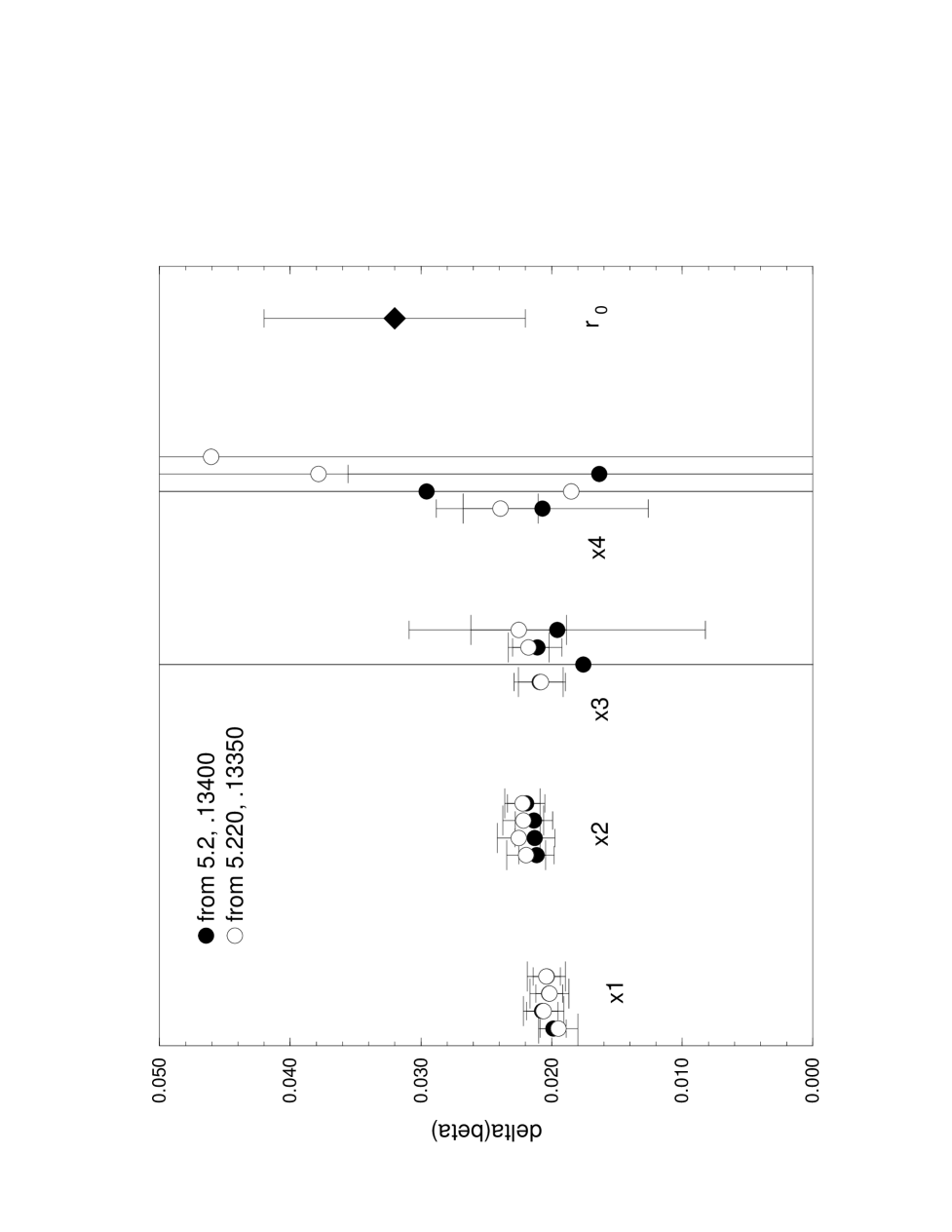
For each loop , we have evaluated the shift required to hold the Wilson loop constant under a change (). The results of this are shown in Figure 1. The values of are similar to each other and to that for the average plaquette measured above. There is not much evidence of a shift increasing with the loop size, although the loops show a higher trend than the plaquette value. One sees little evidence of mis-matching above the level of a standard deviation.
If this result (same ) was reproduced for all gauge invariant loops and all linear combinations thereof, we would conclude that the static potential, and hence the lattice spacing, would be identical at the matched points (40) and (42). This would realise our initial objective of defining curves of constant effective volume. However, it cannot be that all fixed- curves emanating from a finite reference point coincide. Moving from this point, in one direction we approach the quenched limit and in the other the chiral limit. We expect that different observables will be more or less sensitive to the effects of quenching. For example, the mass of a vector meson will probably change by less than 10% as the chiral limit is reached in the full theory as compared to its quenched value. On the other hand, the string tension should change from the lattice equivalent of 440 Mev to zero, eventually. We study the static potential in the next section.
E Potential and
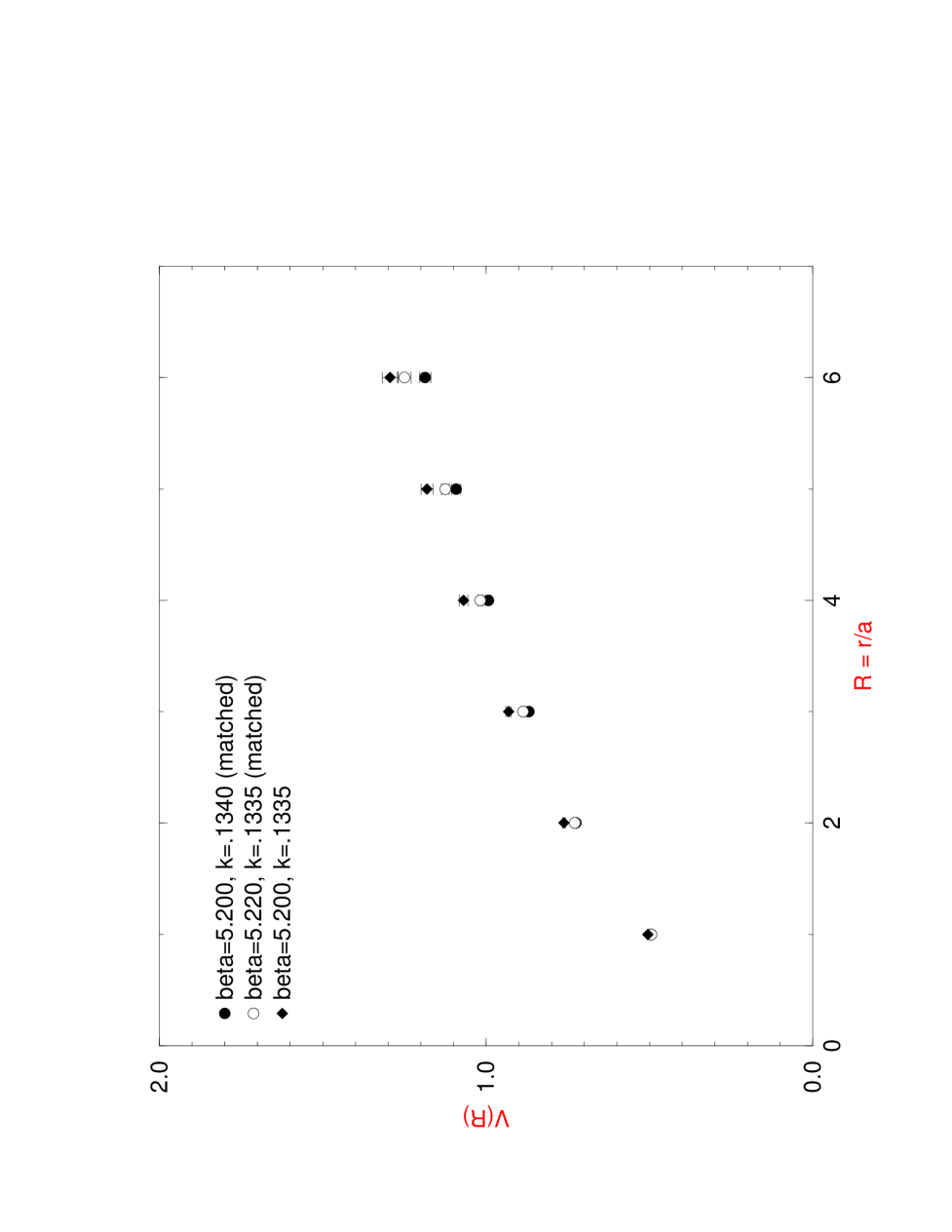
We have used the methods of [12] to measure the potential on each of the main ensembles studied. Since these are on lattices, there are strong finite size effects present in and at the parameter values of interest. However, for the present purpose this is of little consequence. In the variational methods of [12] one constructs ‘fuzzed’ loops from a variety of spatial paths and employs transfer matrix methods to extract energy eigenvalues. The potential values were estimated by taking weighted averages of the effective masses at large time. We took care to use the same procedures on all ensembles. Errors were estimated by bootstrap.
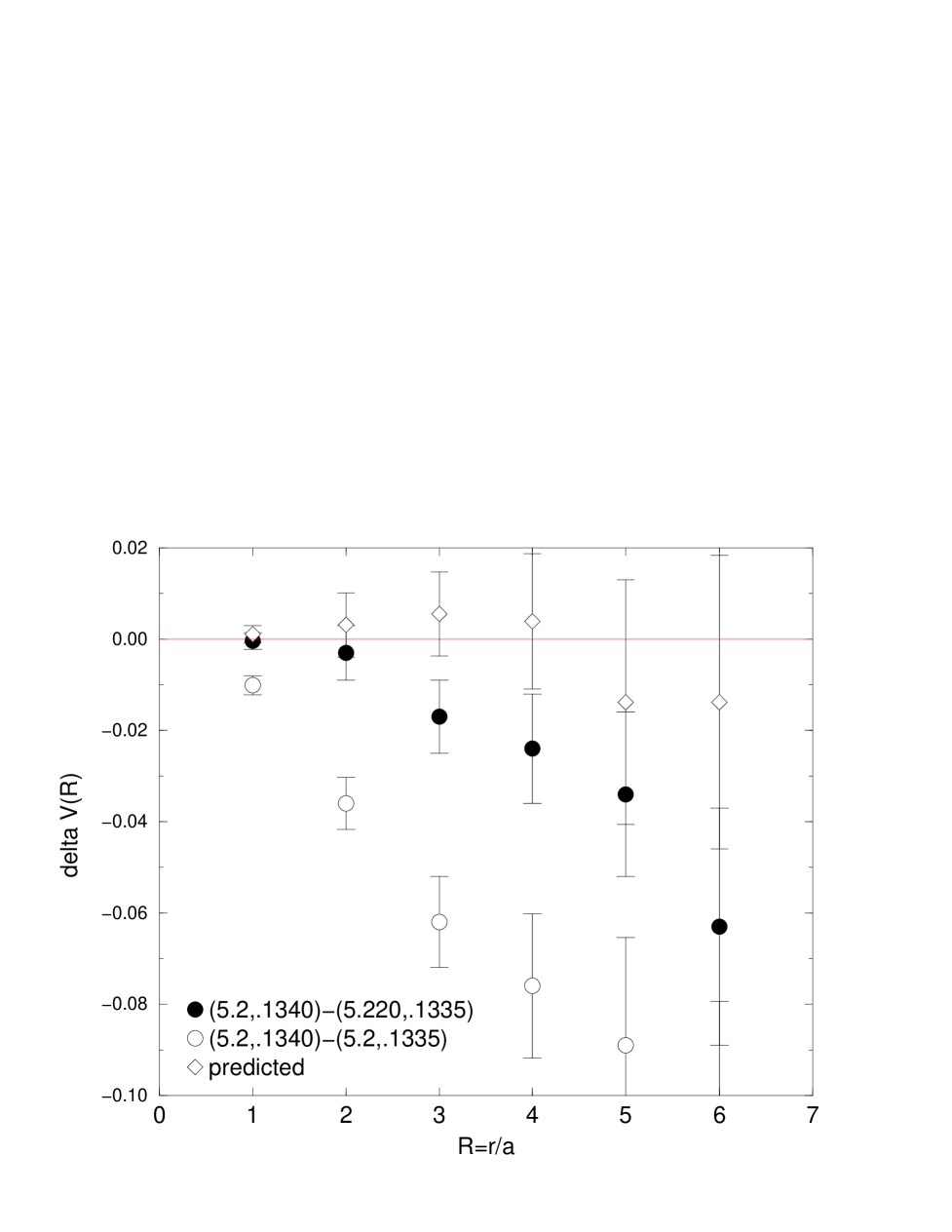
Figure 2 shows the static potential at the matched points (40) and (42). The values are in good agreement at short distances but show a systematic divergence at larger separations. Figure 3 shows more clearly the difference between the potentials . There appears to be a systematically increasing difference at larger distance. For comparison, the figure also shows where there has been a shift in but no compensating change in . There is clear disagreement at all distances, as expected.
The remaining set of points in Figure 3 shows the prediction for from the reference ensemble at using (4) to first order. Within the large statistical errors, the predicted difference is indeed compatible with zero. This demonstrates that where matching has been done only approximately (in this case with ) an observable can still be reliably estimated at another nearby point of interest.
From the comparison of the directly simulated points, we conclude that matching the plaquette is not equivalent to matching the long range potential. Note that no corrections have been made for lattice artifacts at short distances but these are expected to be similar in each case.
From the potential measurements represented in Figure 2 we can extract corresponding values of [4] and, hence, lattice spacing using . These are shown in Table V. In finding , we have calculated interpolated values of the static force via Newtonian 5-point interpolation of the potential. As usual, errors were computed via bootstrap. The same procedures were used for each ensemble.
From Table V, we see that the lattice volume at the matched points is similar although that at the heavier quark mass is perhaps one standard deviation larger. This is a reflection of the observation made above that the potentials diverge at large separations due to their different slopes. We have attempted to estimate required to match the mean values of the lattice spacings. In the last three rows of Table V, we show the lattice spacing predicted from the reference ensemble via (4) for shifts of , and to go with the shift of . The spacing predicted for agrees well with that measured by direct simulation (previous line). From this value and those corresponding to and we estimate that the optimal matching for the lattice spacing (as opposed to the plaquette) would be . This value is compared with those corresponding to the various Wilson loops in Figure 1.
We conclude that the constant lattice volume curve (as defined by ) may indeed differ from that corresponding to constant plaquette value. With only 40 configurations, the evidence is of marginal statistical significance. As a cross-check we measured directly from a simulation at . See Table V. The result was compatible with the prediction and with the matched ensemble from which the prediction was made. Again, the statistical significance is not high.
We have also measured on quenched configurations at , the point which is predicted and verified to have matched values of , and at , close to the point where is expected to match. Results are shown in Table III. As expected, the lattice spacing does not match at but is close to matching at . The shift required to match is some larger than that required to match .
F Hadron correlators
Finally in this section, we present results from matching lattice pion correlators. This test is made more practicable by recent advances in measuring hadron correlators with good statistical precision on a single gauge configuration [13]. We have made measurements of the local pion correlator on the reference ensemble and calculated the corresponding shifts. That is, for each value of , we estimate the shift required to keep constant for the test shift. Results are presented Table VI where they are compared with examples of other observables. At short time separations ( and ) we find values compatible with that for the plaquette. At large values of the results are overwhelmed by noise and we are unable to draw conclusions. However there are indications that for increasing the shift required in is also increasing. See, for example the correlator for and corresponding effective mass values which are also shown in the table:
| (45) |
Clearly one requires greater statistics to confirm these trends, but they are consistent with those inferred from the results presented above. A compilation of shifts for sample loops, and are shown in Figure 4.
Note that the effective mass values involved in this test are very far from those of a physical pion.
V Further applications
The above matching technology has a variety of potential uses including the following.
A Parallel tempering
Parallel tempering (PT) is an improved Monte–Carlo method originally proposed by Hukushima et al [14] to improve simulations of spin glasses. It was further discussed by Marinari et al in [15] and [16] who suggested its use in Lattice QCD. Recently Boyd [17] applied the technique to lattice QCD with staggered fermions and found evidence that Parallel Tempering did help decorrelate long distance observables.
Parallel tempering essentially consists of running several independent simulations in parallel and with different parameters. Each such simulation produces a set of configurations which is distributed according to the probability distribution dictated by the simulation action and parameters. The PT algorithm exploits the fact that these distributions may have an overlap and occasionally attempts to swap configurations between ensembles. Acceptance of the swap is controlled by a Metropolis style acceptance step.
This is the same situation described by the matching criterion M3 in section II. From another viewpoint, the distance between the actions in matching criterion M2 can be related to the acceptance rate of the swaps in a parallel tempering algorithm.
In [17], tempering was carried out in the quark mass only. All the ensembles had the same value of . Furthermore, the quark masses had to be spaced quite closely together to obtain a reasonable swap acceptance rate. With the matching technology presented in this paper, it is possible to temper in both and the quark mass. This may allow one to perform PT along a curve of approximately constant volume, and at a such a separation between ensembles that one might use some of the tempering ensembles to perform chiral extrapolations. Alternatively, one might be able to simulate with ensembles suitably chosen to improve the decorrelation properties of the system as a whole. A detailed investigation into PT using the matching technology is being conducted by us and the full results will be reported elsewhere [18].
B Approximate algorithms
In [5] we demonstrated how the parameters of approximate algorithms could be tuned according to the criteria M1, M2 or M3 described above. In subsequent tests [7], we showed that approximate algorithms based on a few Wilson loops only, were unlikely to produce a very accurate approximation, at least in the sense of M3 where the approximate action acts as the guide within an exact algorithm. The variance of the difference between the two extensive quantities remains unacceptably large on lattices of a useful size. It is, however, still of considerable interest to design approximate or model actions which improve on the quenched approximation by encapsulating at least some of the additional physics implied by dynamical quarks.
An alternative route to an exact algorithm might be to make use of the Lanczos quadrature approximation of section III for part of the effective action and gauge invariant loops as above for the remainder. The trial configurations would be generated by the loop part of the action and an accept/reject step based on the Lanczos part. The technology of section II can be used to tune the loop part together with the Lanczos part to match the exact action. As a simple example of this approach, consider an approximate action defined such that (c.f. (7))
| (46) |
where is the approximation to as described in section III but using only Lanczos iterations. The loop part of the effective action is just a single plaquette in this example. In a standard Metropolis update this action would only be viable if was considerably smaller than the typical values (90) required to estimate the true action, and sufficient account was taken of the short range fluctuations by having a properly tuned gauge loop part. This approximation is similar in spirit to that advocated in [19, 20] where it is argued that a truncated sum of low-lying eigenvalues can reproduce the gross behaviour of the fermion determinant. In the present scheme, we are able to obtain a particularly efficient approximation to the trace log by using the optimal weighting determined by the Gaussian quadrature rule. We have conducted preliminary tests of these ideas by measuring the shift required to compensate for a truncation to Lanczos iterations. In a simple test which matched the average plaquette, the shift in was reduced by a factor of in changing from (quenched) to , for example. The correspond residual variance (after matching) also dropped by a factor of around . For increasing , the shift rapidly becomes compatible with zero at the level of statistical accuracy implied by the number of noise vectors used (). This demonstrates that the Lanczos quadrature approach gives a very efficient estimator for the trace log. It will be worth exploring whether the long range modes described by such an approximation can be combined with a suitably tuned gauge loop action describing short range modes so as to achieve a practical exact algorithm.
VI Conclusions
We have proposed a strategy for dynamical quark simulations in which the effective lattice volume is held fixed while the effects of progressively lighter sea quarks are investigated. Possible algorithms for accomplishing this have been presented and the results of tests discussed. In particular, we have presented results using an efficient stochastic estimator of the fermion determinant and quantities related to it. These include estimates of the constant lattice spacing curves at relevant points in the plane for lattice QCD using a non-perturbatively improved action. We have demonstrated that the work involved in determining such curves via our differential stochastic methods is considerably less than that required to establish them by direct simulation. Further applications of these techniquess have been discussed.
ACKNOWLEDGMENTS
Computational resources for this work were in part provided by the HPCI inititaive of EPSRC under grant GR/K41663. Alan Irving and James Sexton are grateful to the British Council/ Forbairt Joint Research Scheme for travel support. James Sexton would also like to thank Hitachi Dublin Laboratory for its support.
REFERENCES
- [1] S. Güsken, Nucl. Phys. B (Proc. Suppl.) 63A-C (1998) 16.
- [2] M. Talevi,UKQCD collaboration Nucl. Phys. B (Proc. Suppl.) 63A-C (1998) 227.
- [3] C. A. Allton, UKQCD collaboration, in preparation.
- [4] R. Sommer, Nucl. Phys. B411 (1994) 839.
- [5] A. C. Irving and J. C. Sexton, Phys. Rev. D55 (1997) 5456.
- [6] Z. Bai, M. Fahey and G. Golub, ‘Some Large Scale Matrix Computation Problems’, Technical report SCCM-95-09, School of Engineering, Stanford University (1995).
- [7] A. C. Irving, J. C. Sexton and E. Cahill, Nucl. Phys. B (Proc. Suppl.) 63A-C (1998) 967
- [8] J. C. Sexton and D. H. Weingarten, Nucl. Phys. B (Proc. Suppl.) 42 (1995) 361; J. C. Sexton and D. H. Weingarten, preprint heplat/9411029.
- [9] B. Sheikholeslami and R. Wohlert, Nucl. Phys. B259 (1985) 572.
- [10] K. Jansen and R. Sommer, hep-lat/9709022.
- [11] E. Cahill, J. C. Sexton and A. C. Irving, in preparation.
- [12] S. J. Perantonis and C. Michael, Nucl. Phys. B347 (1990) 854.
- [13] C. Michael and J. Peisa…
- [14] K. Hukushima, J. Nemoto, cond-mat/9512035.
- [15] E. Marinari, cond-mat/9612010
- [16] E. Marinari, G. Parisi, J. J. J. Ruiz-Lorenzo, cond-mat/9701016
- [17] G. Boyd, hep-lat/9712012
- [18] A. C. Irving, J. C. Sexton, B. Joó, UKQCD collaboration, in preparation.
- [19] W. Bardeen, A. Duncan, E. Eichten and H. Thacker, Nucl. Phys. B (Proc. Suppl.) 63A-C (1998) 811
- [20] A. Duncan, E. Eichten and H. Thacker, FERMILAB-PUB-98/181-T, hep-lat/9806020.

| Parameter | Description | Value |
| number of HMC steps per trajectory | 50 | |
| number of sweeps in the HMC solver (e.g.BiCGStab) | 300 | |
| HMC trajectory acceptance | 0.75 | |
| autocorrelation time in trajectories | 30 | |
| number of noise vectors (section III) | 80 | |
| number of Lanczos iterations | 90 |
| (average plaquette) | |||
|---|---|---|---|
| traj | config | |||||
| sweeps | ||||||
| Loop | No. of links | Link steps |
|---|---|---|
| 1 | 4 | (+1,+2,-1,-2) |
| 2 | 6 | (+1,+1,+2,-1,-1,-2) |
| 3 | 6 | (+1,+2,+3,-2,-1,-3) |
| 4 | 6 | (+1,+2,+3,-1,-2,-3) |
| a fm | |||
| direct simulation | |||
| by HMC | |||
| pred. | |||
| from | |||
| using (4) |
| Measurement | Value at | |
|---|---|---|