HLRZ-98/22
BUGHW-SC-98/4
WUP-98/20
Preconditioning of Improved and “Perfect” Fermion Actions

Abstract

We construct a locally-lexicographic SSOR preconditioner to accelerate the parallel iterative solution of linear systems of equations for two improved discretizations of lattice fermions: (i) the Sheikholeslami-Wohlert scheme where a non-constant block-diagonal term is added to the Wilson fermion matrix and (ii) renormalization group improved actions which incorporate couplings beyond nearest neighbors of the lattice fermion fields. In case (i) we find the block ll-SSOR-scheme to be more effective by a factor $\approx 2$ than odd-even preconditioned solvers in terms of convergence rates, at $\beta=6.0$. For type (ii) actions, we show that our preconditioner accelerates the iterative solution of a linear system of hypercube fermions by a factor of 3 to 4.

1 Introduction

Traditionally, simulations of lattice quantum chromodynamics (QCD) were based on nearest-neighbor finite difference approximations of the derivatives of classical fields. It is a general observation made in both quenched and full QCD that results from lattices with a resolution $>0.1$ fm suffer from considerable discretization errors, see e. g. Ref. [2]. Even optimistic estimates expect an increase in costs of full QCD simulations $\propto a^{-6}$ as the lattice spacing $a$ is decreased [3]..

The Wilson fermion formulation is appropriate with respect to flavor symmetry, but plagued by discretization errors of ${\cal O}(a)$. These effects have been found to be sizeable e. g. in a compilation of quenched world data for quark masses [5] and in the determination of the renormalized quark mass, exploiting the PCAC relation in the Schrödinger functional [6, 7].

In lattice QCD, the extraction of physical continuum results requires to approach two limits: the chiral limit defined as the point in parameter space where the pion mass vanishes, and the continuum limit defined by vanishing lattice spacing $a$. The chiral limit amounts to an increase of the inverse pion mass (the correlation length $\xi_{\pi}$) in lattice units towards infinity. The lattice volume, i. e. the number of sites, must be increased accordingly, in order to control finite size effects. At this point, simulations of QCD with dynamical fermions encounter the problem of solving the fermionic linear system $MX=\phi$, where $M$ is the fermion matrix—a compute intensive task.

The second step, moving towards the continuum limit, requires to decrease the lattice spacing $a$. The two issues are related: if one would be able to get reliable results at larger lattice spacing, one could avoid dealing with prohibitively fine physical lattice resolutions on large physical volumes. On the classical level, one might just use higher order derivative terms in the fermion action in order to push finite-$a$-effects to higher orders. But quantum effects will largely spoil the intended gains.

At present, there are two major trends to improve the fermionic discretization. One approach follows Symanzik’s on-shell improvement program [11]. Irrelevant (dimension 5) counter terms are added to both, lattice action and composite operators in order to avoid ${\cal O}(a)$ artifacts. A particularly simple and hence preferred scheme is the Sheikholeslami and Wohlert action (SWA) [10], where the Wilson action is modified by adding a local term, the so-called clover term. Hereby, the amount of storage is doubled. The clover term is sufficient, in principle, to cancel the ${\cal O}(a)$ errors in the action, provided that a constant $c_{SW}$ is tuned suitably. The hope is to reach the continuum limit for a given scaling quantity $Q$ as $Q(a)=Q_{continuum}+{\cal O}(a^{2})$, i. e. without ${\cal O}(a)$ contamination. The development of a non-perturbative tuning procedure has been documented in a series of papers, see Refs. [6, 7, 12, 13].

Another promising ansatz is based on Wilson’s renormalization group [14]. It goes under the name perfect actions. Perfect lattice actions are located on renormalized trajectories in parameter space that intersect the critical surface (at infinite correlation length) in a fixed point of a renormalization group transformation. By definition, perfect actions are free of any cut-off effects, therefore they represent continuum physics at any lattice spacing $a$.

In practice, perfect actions can best be approximated for asymptotically free theories starting from fixed point actions. Such fixed point actions can be identified in a multi-grid procedure solely by minimization, without performing functional integrals. Thus, the task reduces to a classical field theory problem. The fixed point action then serves as an approximation to a perfect action at finite correlation length; this is a so-called classically perfect action [15]. However, even in this approximation the couplings usually extend over an infinite range, so for practical purposes a truncation to short distances is unavoidable. In such schemes of ‘truncated perfect actions’ (TPA) one is forced to give up part of the original quest for perfectness, for reasons of practicability.

It goes without saying that SWA and TPA can prove their full utility only after combination with state-of-the-art solvers in actual parallel implementations. In the recent years, the inversion of the standard Wilson fermion matrix could be accelerated considerably by use of the BiCGStab algorithm [8] and novel parallel locally-lexicographic symmetric successive over-relaxation (ll-SSOR) preconditioning techniques [9].

We start from the hypercube fermion (HF) approximation formulated for free fermions in Ref. [16]. For an alternative variant, see Ref. [18]. In order to meet the topological structure of TPA, we shall follow a bottom-up approach by adding interactions to the free fermion case through hyper-links within the unit-hypercube. This results in 40 independent hyper-links per site and amounts to a storage requirement five times as large as in SWA.

In general, the fermion matrix for both SWA and TPA can be written in the generic form

$$M=D+A+B+\cdots,$$ (1)

where $D$ represents diagonal blocks (containing $12\times 12$ sub-blocks), $A$ is a nearest-neighbor hopping term, while $B$ contains next-to-nearest-neighbor couplings, and so on.

The key point is that one can include into the ll-SSOR process (i) the internal degrees of freedom of the block diagonal term $D$ as arising in SWA and (ii) 2-space, 3-space, and 4-space hyper-links, as present in a TPA like HF.

After reviewing the fermionic matrices for SWA and HF in section 2, we introduce locally lexicographic over-relaxation (ll-SSOR) preconditioning of SWA in section 3. We discuss three variants for the diagonal blocks to be used in block SSOR. In section 4, we shall parallelize block SSOR within an extended ll-SSOR-scheme and we shall discuss the inclusion of the HF into this framework. In section 5, we benchmark the block-ll-SSOR preconditioner on SWA—for several values of $c_{SW}$—in comparison with odd-even preconditioning. Our testbed is a set of quenched configurations on lattices of size $16^{4}$ at $\beta=6.0$ and our implementation machines are a 32-node APE100/Quadrics and a SUN Ultra workstation. Using the HF on a quenched $8^{4}$ system, we compare the SSOR preconditioned version with an non-preconditioned one, for a variety of mass parameters, again at $\beta=6.0$.

2 Improved Fermionic Actions

In this section we briefly review the basics of SWA and TPA. To fix our notation, we write the fermionic lattice action as

$$S_{F}=\sum_{x,y}\bar{\Psi}_{x}M(x,y)\Psi_{y},$$ (2)

where $M$ is the fermion matrix.

2.1 Sheikholeslami-Wohlert Action

For the Wilson fermion action (with Wilson parameter $r=1$), supplemented by the Sheikholeslami-Wohlert term, we have

$$M_{SW}(x,y) = \Big{[}{\mathbf{1}}+\frac{c_{SW}}{2}\kappa\sum_{\mu,\nu}\sigma_{\mu\nu}F_{\mu\nu}(x)\Big{]}\delta_{x,y}$$

$$- \kappa\sum_{\mu}\Big{[}({\mathbf{1}}-\gamma_{\mu})U_{\mu}(x)\delta_{x,y-\hat{\mu}}+({\mathbf{1}}+\gamma_{\mu})U_{-\mu}(x)\delta_{x,y+\hat{\mu}}\Big{]},$$

where $\kappa$ is the standard Wilson hopping parameter, $c_{SW}$ is a parameter that can be tuned to optimize ${\cal O}(a)$ cancellations, and $\hat{\mu}$ is a unit vector.

The ‘local’ clover term consists of $12\times 12$ diagonal blocks. Its explicit structure in Dirac space is given by

$$\frac{1}{2}\sum_{\mu,\nu}\sigma_{\mu\nu}F_{\mu\nu}=\left(\begin{array}[]{cccc}F_{1}&F_{2}&F_{3}&F_{4}\\ F_{2}^{\dagger}&-F_{1}&F_{4}^{\dagger}&-F_{3}\\ F_{3}&F_{4}&F_{1}&F_{2}\\ F_{4}^{\dagger}&-F_{3}&F_{2}^{\dagger}&-F_{1}\\ \end{array}\right)\ ,$$ (4)

with the entries $F_{i}$ being complex $3\times 3$ matrices, which are shorthands for linear combinations of the $F_{\mu\nu}$,

$$\begin{array}[]{cc}F_{1}=-F_{12},&\quad F_{2}=-F_{23}-iF_{13},\\ F_{3}=F_{34},&\quad F_{4}=F_{14}-iF_{24}.\\ \end{array}$$ (5)

$F_{\mu\nu}$ is defined by

$$F_{\mu\nu}:=\frac{i}{8}\left(f_{\mu\nu}-f^{\dagger}_{\mu\nu}\right),$$ (6)

where the clover term $f_{\mu\nu}$ reads

$$f_{\mu\nu}(x) := U_{\mu}(x)U_{\nu}(x+\hat{\mu})U^{\dagger}_{\mu}(x+\hat{\nu})U^{\dagger}_{\nu}(x)$$

$$+ U_{\nu}(x)U^{\dagger}_{\mu}(x-\hat{\mu}+\hat{\nu})U^{\dagger}_{\nu}(x-\hat{\mu})U_{\mu}(x-\hat{\mu})$$

$$+ U^{\dagger}_{\mu}(x-\hat{\mu})U^{\dagger}_{\nu}(x-\hat{\mu}-\hat{\nu})U_{\mu}(x-\hat{\mu}-\hat{\nu})U_{\nu}(x-\hat{\nu})$$

$$+ U^{\dagger}_{\nu}(x-\hat{\nu})U_{\mu}(x-\hat{\nu})U_{\nu}(x+\hat{\mu}-\hat{\nu})U^{\dagger}_{\mu}(x).$$

The Wilson-Sheikholeslami-Wohlert matrix exhibits the well known $\gamma_{5}$ symmetry

$$\gamma_{5}\,M_{SW}\gamma_{5}=M_{SW}^{\dagger},$$ (7)

with the eigenvalues of $M_{SW}$ coming in complex-conjugate pairs.

2.2 Hypercube Fermions

The physical properties of a given lattice action remain unaltered under a block variable renormalization group transformation (RGT). As a simple example, we can divide the (infinite) lattice into disjoint hypercubic blocks of $n^{d}$ sites each and introduce new variables living on the centers of these blocks (block factor $n$ RGT). Then the RGT relates

$$\phi^{\prime}_{x^{\prime}}\sim\sum_{x\in x^{\prime}}\phi_{x},$$ (8)

where $\phi$ and $\phi^{\prime}$ represent the original and the new lattice fields, respectively. The points $x\in{\mathbb{Z}}^{d}$ are the sites of the original lattice and $x^{\prime}$ are those of the new lattice with spacing $n$. $x\in x^{\prime}$ means that the point $x$ belongs to the block with center $x^{\prime}$.

Now the original action $S[\phi]$ transforms into a new action $S^{\prime}[\phi^{\prime}]$ on the coarse lattice. The latter is determined by the functional integral

$$e^{-S^{\prime}[\phi^{\prime}]}=\int D\phi\ K[\phi^{\prime},\phi]e^{-S[\phi]}.$$ (9)

The kernel $K[\phi^{\prime},\phi]$ has to be chosen such that the partition function and all expectation values remain invariant under the RGT. At the end, one usually rescales the lattice spacing back to 1. In any case, the correlation length in lattice units gets divided by $n$.

For the kernel functional there are many possible choices [19]. A particularly simple choice for the kernel functional is

$$K[\phi^{\prime},\phi]=\prod_{x^{\prime}}\delta\Big{(}\phi^{\prime}_{x^{\prime}}-\frac{\beta_{n}}{n^{d}}\sum_{x\in x^{\prime}}\phi_{x}\Big{)}\ .$$ (10)

Assume that we are on a “critical surface”, where the correlation length is infinite. With a suitably chosen renormalization factor $\beta_{n}$ we obtain—after an infinite number of RGT iterations—a finite fixed point action (FPA) $S^{*}[\phi]$. An FPA is invariant under the RGT. The task of $\beta_{n}$ is the neutralization of the rescaling of the field $\phi^{\prime}$ at the end. The FPA is an example of a perfect lattice action since it is insensitive to a change of the lattice spacing.

Eq. (10) can be generalized, for instance, to a Gaussian form of blocking. For free fermions, a generalization of this type reads (we ignore constant factors in the partition function)

$$e^{-S^{\prime}[\bar{\Psi}^{\prime},\Psi^{\prime}]}=\int D\bar{\Psi}D\Psi e^{-S[\bar{\Psi},\Psi]}$$ (11)

$$\times \exp\Big{\{}-\frac{1}{\alpha}\sum_{x^{\prime}}\Big{[}\bar{\Psi}^{{}^{\prime}}_{x^{\prime}}-\frac{1}{n^{(d+1)/2}}\sum_{x\in x^{\prime}}\bar{\Psi}_{x}\Big{]}\Big{[}\Psi^{{}^{\prime}}_{x^{\prime}}-\frac{1}{n^{(d+1)/2}}\sum_{x\in x^{\prime}}\Psi_{x}\Big{]}\Big{\}}.$$

Here we have already inserted the suitable parameter $\beta_{n}$ and we introduce a new RGT parameter $\alpha$, which is arbitrary. The critical surface requires a fermion mass $m=0$, but we can generalize the consideration to a finite mass.

Assume that we want to perform a number $N$ of RGT iterations. If we start from a small mass $m/(nN)$, then the final mass will be $m$. In the limit $nN\to\infty$ we obtain a perfect action at finite mass. In this context, “perfect” means that scaling quantities do not depend on the lattice spacing, hence they are identical to the continuum values.

For the above transformation (11), this perfect action can be computed analytically in momentum space [20]. The computation simplifies if we let $n\to\infty$, so that $N=1$ is sufficient. Hence we start from the continuum action now, and the perfect action takes the form

$$S^{*}[\bar{\Psi},\Psi] = \frac{1}{(2\pi)^{d}}\int_{-\pi}^{\pi}d^{d}p\ \bar{\Psi}(-p)\Delta^{*}(p)^{-1}\Psi(p)$$

$$\Delta^{*}(p) = \sum_{l\in Z\!\!\!Z^{d}}\frac{\Pi(p+2\pi l)^{2}}{i(p_{\mu}+2\pi l_{\mu})\gamma_{\mu}+m}+\alpha\ ,\quad\Pi(p)=\prod_{\mu=1}^{d}\frac{2\sin(p_{\mu}/2)}{p_{\mu}},$$ (12)

where $\Delta^{*}$ is the perfect propagator. The same perfect action is obtained starting from a variety of lattice actions, in particular from the Wilson fermion action.

In coordinate space we write this action as

$$S^{*}[\bar{\Psi},\Psi]=\sum_{x,r}\bar{\Psi}_{x}[\rho_{\mu}(r)\gamma_{\mu}+\lambda(r)]\Psi_{x+r}.$$ (13)

For $\alpha>0$, where the RGT breaks the chiral symmetry explicitly, the couplings in $\rho_{\mu}$ and $\lambda$ decay exponentially as $|r|$ increases. An exception is the case $d=1$, where they are confined to one lattice spacing for the special choice

$$\alpha=\frac{e^{m}-m-1}{m^{2}}\,.$$ (14)

It turns out that for this choice of $\alpha$ the locality is also excellent in higher dimensions, i. e., the exponential decay of the couplings is very fast. This is important, because for practical purposes the couplings have to be truncated to a short range, and the truncation should not distort the perfect properties too much. An elegant truncation scheme uses periodic boundary conditions over 3 lattice spacings and thus confines the couplings to a unit hypercube. This yields the HF, with spectral and thermodynamic properties still drastically improved compared to Wilson fermions [16, 21].

Of course, it is far more difficult to construct an approximately perfect action for a complicated interacting theory like QCD. However, as a simple ansatz we can just use HF together with the standard gauge link variables. Apart from nearest neighbors, we also have couplings over 2, 3 and 4-space diagonals in the unit hypercube. We connect all these coupled sites by all possible shortest lattice paths, by multiplying the compact gauge fields on the path links. We call this procedure “gauging the HF by hand”. Note that one can connect two sites $x$ and $y$ lying on 2, 3, and 4-space diagonals via $d!$ such shortest lattice paths. We average over all of them to construct the hyper-link, see Fig. 1.

Let us identify the hyper-link $U^{(1)}_{\mu}(x)$ between site $x$ and $x+\hat{\mu}$ with $U_{\mu}(x)$, and let us denote the hyper-link in plane, cube and hyper-cube as $U^{(2)}_{\mu+\nu}(x)$, $U^{(3)}_{\mu+\nu+\rho}(x)$, and $U^{(4)}_{\mu+\nu+\rho+\sigma}(x)$, respectively. Then we can write the corresponding fermion matrix in terms of the hyper-links which can be constructed recursively starting from the gauge links $U^{(1)}_{\mu}$,

$$U^{(d)}_{\mu_{1}+\mu_{2}+\dots+\mu_{d}}(x)= \frac{1}{d}\Big{[} U^{(1)}_{\mu_{1}}(x)\,U^{(d-1)}_{\mu_{2}+\mu_{3}+\dots+\mu_{d}}(x+\hat{\mu}_{1})$$ (15)

$$+ U^{(1)}_{\mu_{2}}(x)\,U^{(d-1)}_{\mu_{1}+\mu_{3}+\dots+\mu_{d}}(x+\hat{\mu}_{2})$$

$$+ \dots$$

$$+ U^{(1)}_{\mu_{d}}(x)\,U^{(d-1)}_{\mu_{1}+\mu_{2}+\dots+\mu_{d-1}}(x+\hat{\mu}_{d})\;\;\Big{]}.$$

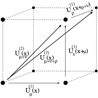
Figure 1: 1-space, 2-space and 3-space hyper-links.

It is convenient to introduce pre-factors which are functions of the HF hopping parameters $\kappa_{i}$ and $\lambda_{i}$, $i=1,\dots,4$, and sums of $\gamma$-matrices:

$$\Gamma_{\pm\mu} = \lambda_{1}+\kappa_{1}(\pm\gamma_{\mu})$$

$$\Gamma_{\pm\mu\pm\nu} = \lambda_{2}+\kappa_{2}(\pm\gamma_{\mu}\pm\gamma_{\nu})$$

$$\Gamma_{\pm\mu\pm\nu\pm\rho} = \lambda_{3}+\kappa_{3}(\pm\gamma_{\mu}\pm\gamma_{\nu}\pm\gamma_{\rho})$$

$$\Gamma_{\pm\mu\pm\nu\pm\rho\pm\sigma} = \lambda_{4}+\kappa_{4}(\pm\gamma_{\mu}\pm\gamma_{\nu}\pm\gamma_{\rho}\pm\gamma_{\sigma})\,.$$ (16)

Note that the $\lambda_{i}$ in eq. (16) differ from $\lambda(r)$ in eq. (13) by a normalization factor $\frac{1}{\lambda_{0}}$. The $\kappa_{i}$ arise from $\rho_{\mu}(r)$ by the same normalization.

The corresponding HF matrix is defined by

$$\scriptscriptstyle\begin{array}[]{rlllllrrrr}M_{HF}(x,y)&=\lambda_{0}\Bigg{\{}\delta_{x,y}\\ +\!\sum\limits_{\mu}\Big{[}\\ \Gamma_{+\mu}&U^{(1)}_{\mu}(x)\delta_{x,y-\hat{\mu}}&{\!\!\!+\!}&\Gamma_{-\mu}U^{(1)}_{-\mu}(x)\delta_{x,y+\hat{\mu}}\;\;\Big{]}\\ \\ +\!\sum\limits_{{\mu}}\!\sum\limits_{{\nu>\mu}}\Big{[}\\ \Gamma_{+\mu+\nu}&U^{(2)}_{+\mu+\nu}(x)\delta_{x,y-\hat{\mu}-\hat{\nu}}&{\!\!\!+\!}&\Gamma_{+\mu-\nu}U^{(2)}_{+\mu-\nu}(x)\delta_{x,y-\hat{\mu}+\hat{\nu}}\\ +\Gamma_{-\mu+\nu}&U^{(2)}_{-\mu+\nu}(x)\delta_{x,y+\hat{\mu}-\hat{\nu}}&{\!\!\!+\!}&\Gamma_{-\mu-\nu}U^{(2)}_{-\mu-\nu}(x)\delta_{x,y+\hat{\mu}+\hat{\nu}}\;\;\Big{]}\\ \\ +\!\sum\limits_{{\mu}}\!\sum\limits_{{\nu>\mu}}\!\sum\limits_{{\rho>\nu}}\Big{[}\\ \Gamma_{+\mu+\nu+\rho}&U^{(3)}_{\mu+\nu+\rho}(x)\delta_{x,y-\hat{\mu}-\hat{\nu}-\hat{\rho}}&{\!\!\!+\!}&\Gamma_{+\mu+\nu-\rho}U^{(3)}_{\mu+\nu-\rho}(x)\delta_{x,y-\hat{\mu}-\hat{\nu}+\hat{\rho}}\\ +\Gamma_{+\mu-\nu+\rho}&U^{(3)}_{\mu-\nu+\rho}(x)\delta_{x,y-\hat{\mu}+\hat{\nu}-\hat{\rho}}&{\!\!\!+\!}&\Gamma_{+\mu-\nu-\rho}U^{(3)}_{\mu-\nu-\rho}(x)\delta_{x,y-\hat{\mu}+\hat{\nu}+\hat{\rho}}\\ +\Gamma_{-\mu+\nu+\rho}&U^{(3)}_{-\mu+\nu+\rho}(x)\delta_{x,y+\hat{\mu}-\hat{\nu}-\hat{\rho}}&{\!\!\!+\!}&\Gamma_{-\mu+\nu-\rho}U^{(3)}_{-\mu+\nu-\rho}(x)\delta_{x,y+\hat{\mu}-\hat{\nu}+\hat{\rho}}\\ +\Gamma_{-\mu-\nu-\rho}&U^{(3)}_{-\mu-\nu+\rho}(x)\delta_{x,y+\hat{\mu}+\hat{\nu}-\hat{\rho}}&{\!\!\!+\!}&\Gamma_{-\mu-\nu-\rho}U^{(3)}_{-\mu-\nu-\rho}(x)\delta_{x,y+\hat{\mu}+\hat{\nu}+\hat{\rho}}\;\;\Big{]}\\ \\ +\!\sum\limits_{{\mu}}\!\sum\limits_{{\nu>\mu}}\!\sum\limits_{{\rho>\nu}}\!\sum\limits_{{\sigma>\rho}}\Big{[}\\ \Gamma_{+\mu+\nu+\rho+\sigma}&U^{(4)}_{\mu+\nu+\rho+\sigma}(x)\delta_{x,y-\hat{\mu}-\hat{\nu}-\hat{\rho}-\hat{\sigma}}&{\!\!\!+\!}&\Gamma_{+\mu+\nu+\rho-\sigma}U^{(4)}_{\mu+\nu+\rho-\sigma}(x)\delta_{x,y-\hat{\mu}-\hat{\nu}-\hat{\rho}+\hat{\sigma}}\\ +\Gamma_{+\mu+\nu-\rho+\sigma}&U^{(4)}_{\mu+\nu-\rho+\sigma}(x)\delta_{x,y-\hat{\mu}-\hat{\nu}+\hat{\rho}-\hat{\sigma}}&{\!\!\!+\!}&\Gamma_{+\mu+\nu-\rho-\sigma}U^{(4)}_{\mu+\nu-\rho-\sigma}(x)\delta_{x,y-\hat{\mu}-\hat{\nu}+\hat{\rho}+\hat{\sigma}}\\ +\Gamma_{+\mu-\nu+\rho+\sigma}&U^{(4)}_{\mu-\nu+\rho+\sigma}(x)\delta_{x,y-\hat{\mu}+\hat{\nu}-\hat{\rho}-\hat{\sigma}}&{\!\!\!+\!}&\Gamma_{+\mu-\nu+\rho-\sigma}U^{(4)}_{\mu-\nu+\rho-\sigma}(x)\delta_{x,y-\hat{\mu}+\hat{\nu}-\hat{\rho}+\hat{\sigma}}\\ +\Gamma_{+\mu-\nu-\rho+\sigma}&U^{(4)}_{\mu-\nu-\rho+\sigma}(x)\delta_{x,y-\hat{\mu}+\hat{\nu}+\hat{\rho}-\hat{\sigma}}&{\!\!\!+\!}&\Gamma_{+\mu-\nu-\rho-\sigma}U^{(4)}_{\mu-\nu-\rho-\sigma}(x)\delta_{x,y-\hat{\mu}+\hat{\nu}+\hat{\rho}+\hat{\sigma}}\\ +\Gamma_{-\mu+\nu+\rho+\sigma}&U^{(4)}_{-\mu+\nu+\rho+\sigma}(x)\delta_{x,y+\hat{\mu}-\hat{\nu}-\hat{\rho}-\hat{\sigma}}&{\!\!\!+\!}&\Gamma_{-\mu+\nu+\rho-\sigma}U^{(4)}_{-\mu+\nu+\rho-\sigma}(x)\delta_{x,y+\hat{\mu}-\hat{\nu}-\hat{\rho}+\hat{\sigma}}\\ +\Gamma_{-\mu+\nu-\rho+\sigma}&U^{(4)}_{-\mu+\nu-\rho+\sigma}(x)\delta_{x,y+\hat{\mu}-\hat{\nu}+\hat{\rho}-\hat{\sigma}}&{\!\!\!+\!}&\Gamma_{-\mu+\nu-\rho-\sigma}U^{(4)}_{-\mu+\nu-\rho-\sigma}(x)\delta_{x,y+\hat{\mu}-\hat{\nu}+\hat{\rho}+\hat{\sigma}}\\ +\Gamma_{-\mu-\nu+\rho+\sigma}&U^{(4)}_{-\mu-\nu+\rho+\sigma}(x)\delta_{x,y+\hat{\mu}+\hat{\nu}-\hat{\rho}-\hat{\sigma}}&{\!\!\!+\!}&\Gamma_{-\mu-\nu+\rho-\sigma}U^{(4)}_{-\mu-\nu+\rho-\sigma}(x)\delta_{x,y+\hat{\mu}+\hat{\nu}-\hat{\rho}+\hat{\sigma}}\\[0.0pt] +\Gamma_{-\mu-\nu-\rho+\sigma}&U^{(4)}_{-\mu-\nu-\rho+\sigma}(x)\delta_{x,y+\hat{\mu}+\hat{\nu}+\hat{\rho}-\hat{\sigma}}&{\!\!\!+\!}&\Gamma_{-\mu-\nu-\rho-\sigma}U^{(4)}_{-\mu-\nu-\rho-\sigma}(x)\delta_{x,y+\hat{\mu}+\hat{\nu}+\hat{\rho}+\hat{\sigma}}\\ &\Big{]}\Bigg{\}}.&&\qquad\qquad\qquad\qquad\qquad\qquad\qquad(\ref{HFMATRIX})\end{array}\displaystyle$$

The sums in eq. (2.2) run over four different directions for two 1-space links, six directions for four 2-space links, four directions for eight 3-space links, and one direction for the sixteen 4-space links. Altogether 80 hyper-links contribute.

With each path of the free HF, a $\gamma$-matrix is associated. We have chosen the $\gamma$-matrices so that they add up to produce an effective $\Gamma$, see eq. (16), which is associated with a given hyper-link.

The 1-space links $U^{(1)}_{\mu}(x)$ are identical to the hermitean-conjugate links in negative direction, $U^{\dagger(1)}_{-\mu}(x+\hat{\mu})$, and this feature also holds for the hyper-links, e. g.,

$$U^{\dagger(d)}_{\mu_{1}+\mu_{2}+\dots+\mu_{d}}(x)=U^{(d)}_{-\mu_{1}-\mu_{2}-\dots-\mu_{d}}(x+\hat{\mu}_{1}+\hat{\mu}_{2}+\dots+\hat{\mu}_{d}).$$ (17)

Therefore, only one half of the hyper-links have to be stored in the implementation of the HF.

As in case of Wilson fermions, the HF matrix exhibits the “$\gamma_{5}$ symmetry”,

$$\gamma_{5}\,M_{HF}\gamma_{5}=M_{HF}^{\dagger},$$ (18)

i. e., $M_{HF}$ is non-hermitean but its eigenvalues come in complex-conjugate pairs.

The off-diagonal elements (“hopping parameters”) $\kappa_{i}$ and $\lambda_{i}$ are shown as functions of the mass $m$ in Fig. 2.

Figure 2: The vector “hopping parameters” $\kappa_{i}$, and the scalar “hopping parameters” $\lambda_{i}$ as functions of the mass $m$.

3 Block SSOR Preconditioning

Preconditioning a linear system

$$M\psi=\phi$$ (19)

amounts to selecting two regular matrices $V_{1}$ and $V_{2}$, which act as a left and a right preconditioner, respectively. This means that we consider the modified system

$$V_{1}^{-1}MV_{2}^{-1}\tilde{\psi}=\tilde{\phi},\enspace\mbox{where }\tilde{\phi}:=V_{1}^{-1}\phi,\;\tilde{\psi}:=V_{2}\psi.$$ (20)

The spectral properties of the preconditioned matrix $V_{1}^{-1}MV_{2}^{-1}$ depend only on the product $V_{1}V_{2}$, but not on the manner how it is factorised into $V_{1}$ and $V_{2}$. For a good choice, the number of iteration steps required for solving eq. (20) by Krylov subspace methods (such as BiCGStab) can be reduced significantly, compared to the original system (19).

In this paper, we consider block SSOR preconditioning. Let $M=D-L-U$ be the decomposition of $M$ into its block diagonal part $D$, its (block) lower triangular part $-L$ and its (block) upper triangular part $-U$. Given a relaxation parameter $\omega\not=0$, block SSOR preconditioning is then defined through the choice

$$V_{1}=\left(\frac{1}{\omega}D-L\right)\left(\frac{1}{\omega}D\right)^{-1},\enspace V_{2}=\frac{1}{\omega}D-U\;.$$ (21)

It is important that block SSOR preconditioning is particularly cheap in terms of arithmetic costs due to the Eisenstat trick [22], which is based on the identity

$$\frac{1}{\omega}D\left(\frac{1}{\omega}D-L\right)^{-1}(D-L-U)\left(\frac{1}{\omega}D-U\right)^{-1}$$

$$= \frac{1}{\omega}D\left\{\left(\frac{1}{\omega}D-L\right)^{-1}\left[{\mathbf{1}}+\left(\frac{\omega-2}{\omega}D\right)\left(\frac{1}{\omega}D-U\right)^{-1}\right]+\left(\frac{1}{\omega}D-U\right)^{-1}\right\}$$

$$= \left({\mathbf{1}}-\omega LD^{-1}\right)^{-1}\left[{\mathbf{1}}+(\omega-2)\left({\mathbf{1}}-\omega UD^{-1}\right)^{-1}\right]+\left({\mathbf{1}}-\omega UD^{-1}\right)^{-1}.$$

Therefore, the matrix-vector product with the preconditioned matrix, $z=V^{-1}_{1}MV^{-1}_{2}x$, can be computed according to Algorithm 1.

solve $({\mathbf{1}}-\omega UD^{-1})y=x$

compute $w=x+(\omega-2)y$

solve $({\mathbf{1}}-\omega LD^{-1})v=w$

compute $z=v+y$

Alg. 1 Matrix-vector product for the preconditioned system.

Here the matrices ${\mathbf{1}}-\omega UD^{-1}$ and ${\mathbf{1}}-\omega LD^{-1}$ are (non-block) lower and upper triangular, respectively. This means that solving the corresponding linear systems amounts to a simple forward and backward substitution process. Algorithm 2 gives a detailed description of the forward substitution for solving $({\mathbf{1}}-\omega LD^{-1})v=w$. Here we denote the block components of the vectors $v,w$ and the matrices $D,L$ as $v_{i},w_{i}$ and $D_{ii}$, $L_{ij}$. The backward substitution for $({\mathbf{1}}-\omega UD^{-1})y=x$ can be carried out analogously.

for $i=1$ to $N$
	$v_{i}=w_{i}+\sum_{j=1}^{i-1}L_{ij}s_{j}$
	$s_{i}=\omega D_{ii}^{-1}v_{i}$

Alg. 2 Forward substitution.

Assuming that the blocks $D_{ii}$ of $D$ are dense and that their inverses have been pre-computed, we see that one iteration step in the above algorithm is exactly as expensive as a direct multiplication with the matrix $D-L$ (except for the additional multiplication with $\omega$). A similar relation holds for the backward substitution and the multiplication with $D-U$. Note that the two multiplications with $D-L$ and $D-U$ are as expensive as one multiplication with the whole matrix $M$ plus one additional multiplication with $D$. This allows us to quantify exactly the work required when using block SSOR preconditioning with the Eisenstat trick.

• Initialization: the inverses $D^{-1}_{ii}$ of all diagonal blocks of the block diagonal matrix $D$ must be pre-computed before the iteration starts. We also assume that these inverses are already scaled by the factor $\omega$ in the initialization.

• Iteration: each iterative step requires additional arithmetic work equivalent to one matrix-vector multiplication with the matrix $D$ plus one vector scaling (with factor $\omega-2$) and two vector summations.

In SU(3) lattice gauge theory, a natural choice for the block diagonal matrix $D$ takes each block $D_{ii}$ to be of dimension 12, corresponding to the 12 variables residing at each lattice point. In this work, we will consider this choice, denoted as $D^{(12)}$, as well as the three generic options $D^{(6)}$, $D^{(3)}$ and $D^{(1)}$, where the diagonal blocks are of dimension 6, 3 and 1, respectively. The choices $D^{(6)}$ and $D^{(3)}$ also appear ‘natural’—at least within the SWA framework—since a diagonal block of $D^{(12)}$ carries the structure of eq. (4). Accordingly, ignoring the parameters $\kappa$ and $c_{SW}$, four consecutive $3\times 3$ blocks in $D^{(3)}$ are given by ${\mathbf{1}}+F_{1}$, ${\mathbf{1}}-F_{1}$, ${\mathbf{1}}+F_{1}$, ${\mathbf{1}}-F_{1}$ and two consecutive $6\times 6$ diagonal blocks in $D^{(6)}$ are identical and given by

$$\left(\begin{array}[]{cc}{\mathbf{1}}+F_{1}&F_{2}\\ F_{2}^{\dagger}&{\mathbf{1}}-F_{1}\end{array}\right)\;.$$ (23)

Table 1 quantifies the arithmetic effort for computing a matrix-vector product with each of the matrices $D^{(12)}$, $D^{(6)}$, $D^{(3)}$ and $D^{(1)}$. We count this effort in units of cflops, which represent one multiplication of complex numbers followed by one summation. The table also quotes estimates for the arithmetic work to compute the inverse of each of these matrices in units of matrix-vector multiplies (MVM). Precise numbers will depend on the particular algorithm chosen for the inversion. The estimates in Table 1 are based on a particularly efficient way for computing the inverse, which uses Cramer’s rule on $3\times 3$ blocks and which exploits the additional block structure within each of the $D^{(6)}_{ii}$ and $D^{(12)}_{ii}$.

The percentages given in brackets quantify these numbers in terms of the cost for a single matrix-vector multiply with $M$. Referring to our previous discussion, they specify the additional cost for (block) SSOR preconditioning. $V$ denotes the lattice volume and one matrix-vector multiplication with $M$ is counted with $528V$ cflops.

Table 1: Arithmetic cost for different sizes of the diagonal blocks. $V$ is the lattice volume.

	$D^{(12)}$	$D^{(6)}$	$D^{(3)}$	$D^{(1)}$
MVM (in cflops)	144$V$ ($27.2\%$)	72$V$ ($13.6\%$)	36$V$ ($6.8\%$)	$V$ ($0.2\%$)
inverse (in MVM)	10	2.5	2	1

4 Parallelization

In the fermion equation (19), we have the freedom to choose any ordering for the lattice points $x$. Different orderings yield different matrices $M$, which are permutationally similar to each other. One matrix can be retrieved from the other one by the transformation $M\rightarrow P^{\dagger}MP$, where $P$ is a permutation matrix. In general, the quality of the block SSOR preconditioner depends on the ordering scheme.

On the other hand, the ordering of the lattice points also determines the degree of parallelism within the forward (and backward) substitutions as described in Algorithm 3. Usually, there is a trade-off between the parallelism a given ordering allows for, and the efficiency of the corresponding SSOR preconditioning.

In an earlier paper [9], we have shown that for the non-block SSOR preconditioner and the Wilson fermion matrix one can use a locally lexicographic ordering on parallel computers supporting grid topologies, so that the resulting SSOR preconditioner parallelizes nicely while significantly outperforming the standard odd-even preconditioner. The purpose of this section is to show that this is also possible for the block SSOR preconditioners considered here, even for situations where $M$ represents couplings beyond nearest-neighbor lattice points.

Let $n(x)$ denote the set of all lattice points a given site $x$ is coupled to. For example, $n(x)=\{y\mid y=x\pm\hat{\mu},~{}\mu=1,\ldots,4\}$ for the nearest-neighbor coupling, $n(x)=\{y\neq x\mid\sum_{\mu=1}^{4}|x_{\mu}-y_{\mu}|\leq 2\}$ for nearest and next-to-nearest neighbor couplings, or $n(x)=\{y\neq x\mid|x_{\mu}-y_{\mu}|\leq 1,~{}\mu=1,\dots,4\}$ for the hypercube couplings.

We now re-formulate the forward substitution of Algorithm 2 for this generalized situation. We assume an overall natural partitioning of $M$ into sub-blocks of dimension 12 (corresponding to the 12 variables at a given lattice point), and we use the lattice positions $x,y$ as indices for those blocks. By $D$ we denote any of the matrices $D^{(12)},\ldots,D^{(1)}$, so $D_{xx}$ stands for a diagonal block of dimension $12\times 12$. It is fully occupied in the case $D=D^{(12)}$, whereas in case $D=D^{(6)}$ it consists of two $6\times 6$ diagonal blocks, etc. We also use the relation $x\leq_{o}y$ between lattice points to denote that $x$ has been numbered before $y$ with respect to a given ordering $o$.

for all lattice positions $x$ in a given ordering $o$
	$v_{x}=w_{x}+\sum_{y\in n(x),\;y\leq_{o}x}L_{xy}s_{y}$
	$s_{x}=\omega D_{xx}^{-1}v_{x}$

Alg. 3 Generalized forward substitution.

To discuss parallelization, we use the concept of coloring the lattice points. A decomposition of all lattice points into mutually disjoint sets $C_{1},\ldots,C_{k}$ is termed a coloring (with respect to the matrix $M$), if for any $l\in\{1,\ldots,k\}$ the property

$$x\in C_{l}\Rightarrow y\not\in C_{l}\;\mbox{ for all }\;y\in n(x)$$

holds. Associating a different color with each set $C_{l}$, this property means that each lattice point couples with lattice points of different colors only. An associated color ordering first numbers all grid points with color $C_{1}$, then all with $C_{2}$ etc. With such a color ordering we see that the computation of $v_{x}$ for all $x$ of a given color $C_{l}$ can be done in parallel, since terms like $\sum_{y\in n(x),\;y\leq_{o}x}$ involve only lattice points from the preceding colors $C_{1},\ldots,C_{l-1}$.

In the case of nearest-neighbor couplings, the familiar odd-even ordering represents such a coloring with two colors corresponding to the odd and the even sublattice. For the case of the Wilson fermion matrix, we pointed out in [9] that the (non-block) SSOR preconditioned system may be interpreted as a representation of the familiar odd-even reduction process. A similar relation arises in the case of SWA, where the reduced system considered in Ref. [23] is equivalent to the ($12\times 12$ block) SSOR preconditioned matrix with odd-even ordering.

For more complicated couplings like the next-to-nearest neighbor couplings or the HF, it would become increasingly difficult to handle colorings with a minimum number of colors. For example, the hypercube ordering requires at least 16 different colors.

However, aiming at a minimal number of colors is not a good strategy. For example, the odd-even coloring can actually be considered as the ‘worst case’ as far as the quality of the corresponding SSOR preconditioner is concerned [9]. Heuristically, this can be explained as follows: if the number of colors is small, the color sets $C_{l}$ themselves are large, and information is not spread between lattice points of equal color in a forward (or backward) substitution.

Therefore, the right strategy is to search for colorings such that the number $k$ of colors is maximal, while the number of points within each color is still in agreement with the parallelization we are aiming for.

The locally lexicographic ordering, proposed in Ref. [9] for the case of a nearest-neighbor coupling, turns out to be an adequate ordering also for more complicated couplings like next-to-nearest neighbor and hypercube.

To describe this ordering, we assume the processors of the parallel computer to be connected as a 4-dimensional grid $p_{1}\times p_{2}\times p_{3}\times p_{4}$. Note that this includes lower dimensional grids by setting some of the $p_{i}$ to 1. The space-time lattice can be matched to the processor grid in a natural manner, producing a local lattice of size $n^{loc}_{1}\times n^{loc}_{2}\times n^{loc}_{3}\times n^{loc}_{4}$ with $n^{loc}_{i}=n_{i}/p_{i}$ on each processor. Here we assume for simplicity that each $p_{i}$ divides $n_{i}$, and that we have $n^{loc}_{i}\geq 2$ for $i=1,\ldots,4$.

Let us divide the lattice sites into $n^{loc}$ groups where $n^{loc}=n^{loc}_{1}n^{loc}_{2}n^{loc}_{3}n^{loc}_{4}$. Each group corresponds to a fixed position within the local grids and contains all grid points appearing at this position within their respective local grid. Associating a color with each of the groups, we get a coloring in the sense of the definition above, as long as the coupling defined through $M$ is local enough. More precisely, the sets represent a coloring, if for all $y\in n(x)$ the relation $|y_{\mu}-x_{\mu}|<n^{loc}_{\mu}$ holds for $\mu=1,\ldots,4$. For example, we need $n_{\mu}^{loc}\geq 2$ for all $\mu$ for the hypercube couplings and $n_{\mu}^{loc}\geq 3$ for all $\mu$ for the next-to-nearest neighbor couplings.

A locally lexicographic ($ll$) ordering is now defined to be the color ordering, where all points of a given color are ordered after all points with colors, which correspond to lattice positions on the local grid that are lexicographically preceding the given color. In Fig. 3, this amounts to the alphabetic ordering of the colors $a$ – $q$. This example also illustrates the decoupling obtained through that ordering for (2-dimensional) nearest-neighbor and hypercube couplings.

Figure 3: Locally lexicographic ordering and forward solve in 2 dimensions. Nearest-neighbor: straight arrows, hyper-cube couplings: straight and thin diagonal arrows.

The parallel version of the forward substitution in Algorithm 4 with the $ll$-ordering now reads:

for all colors in lexicographic order
	for all processors
		$x:=$ grid point of the given color on that processor
		$v_{x}=w_{x}+\sum_{y\in n(x),\;y\leq_{ll}x}L_{xy}s_{y}$
		$s_{x}=\omega D_{xx}^{-1}v_{x}$

Alg. 4 $ll$-forward substitution.

If the lattice point $x$ is close to the boundary of the local lattice, then the set $n(x)$ will contain grid points $y$ residing in neighboring processors. Therefore, some of the quantities $s_{y}$ will have to be communicated from those neighboring processors. The detailed communication scheme for the case of a nearest-neighbor coupling was given in Ref. [9]. In that case, only the 8 nearest neighbors in the processor grid were involved in the communication. For the more complicated HF couplings, all 80 hypercube neighbors may be involved. For a 3- or 2-dimensional processor grid, this number reduces to 26 resp. 8.

5 Results

The ll-SSOR preconditioning of improved actions has been tested in quenched QCD, for realistic lattice sizes and parameters. For SWA we use the odd-even preconditioner of Ref. [23] as reference. The HF action preconditioner has been implemented only on a scalar machine so far. Work for a parallel implementation is in progress.

5.1 Sheikholeslami-Wohlert Action

We are going to compare results from test runs of ll-SSOR and odd-even preconditioning, both codes being equally well optimized for the multiplication of the SWA fermion matrix. Our investigations are based on a de-correlated set of 10 quenched gauge configurations generated on a $16^{4}$ lattice at $\beta=6.0$. We have taken measurements at 3 values of $c_{SW}$, 0, 1.0 and 1.769. The latter value is the optimal quenched $c_{SW}$ coefficient taken from Ref. [13].

In order to provide both machine independent numbers and real time results on parallel and scalar implementation machines, we will present iteration numbers which (i) are directly proportional to the amount of floating point operations and (ii) real time results from implementations on both the parallel system APE100/Quadrics and a SUN Ultra workstation.

We have applied BiCGStab as iterative solver. The stopping criterion has been chosen as $r=\frac{||MX-\phi||}{||X||}\leq 10^{-6}$. We used a local source. At the end of the computation, we have checked how far the true residuum deviates from the accumulated one. In fact, for ll-SSOR, the accumulated residuum turned out to deviate only slightly from the corresponding true residuum. Moreover, deviations between the solutions $X$ as computed by ll-SSOR and odd-even-preconditioning have been checked. We found the norms of the solution vectors to differ in the range of $10^{-6}$.

In a first step, we have determined the optimal value for the over-relaxation parameter $\omega$ as introduced in eq. (21), see Fig. 4. The $\omega$ dependence of the iteration numbers is measured for $c_{SW}=1.769$ at a given value for the hopping parameter $\kappa=0.1333$. At this value, the fermion matrix is close to criticality.

Figure 4: $\omega$-dependence of ll-SSOR. We plot the gain factor between ll-SSOR and odd-even preconditioning.

In Fig. 4, the results from three diagonal block sizes are overlaid, the $1\times 1$, $3\times 3$, and $6\times 6$ blocks. Only a weak dependence of the iteration numbers on the block size is visible, however. Around $\omega=1.4$ a minimum in iteration numbers is found. We have verified that this number holds for the whole $\kappa$-range investigated and for the other values of $c_{SW}$ as well.

Figure 5: $\kappa$ dependence of ll-SSOR vs. the odd-even preconditioner for three values of $c_{SW}$.

Next we benchmark the ll-SSOR preconditioner against the odd-even preconditioner. In Fig. 5, the iteration numbers are presented as a function of $\kappa$, separately for the three values chosen for $c_{SW}$. We plot the ratio of iteration numbers of the odd-even procedure vs. ll-SSOR. In the last two segments of the figure, three block sizes are overlaid.

The improvement of ll-SSOR compared to the odd-even preconditioned system is rather substantial: close to $m_{c}$, i. e. in the region of interest, a factor up to 2.5 in iteration numbers can be found, with increasing tendency when approaching $\kappa_{c}$. As far as the dependence of the improvement factor on $c_{SW}$ is concerned, one cannot detect a systematic effect. Significant block size dependencies are not visible either. However, in the actual time measurements on APE100 to be shown below, we will find the $3\times 3$ local diagonal block procedure to perform best.

The above results have been achieved on a machine equipped with $p=32$ processors. With $V=65536$ being the number of sites on the lattice the sub-lattices comprise $2048$ sites each. As the regions which are treated independently in the preconditioning process are as large as the size of a sub-lattice assigned to a given processor, the parallelism of the preconditioner follows the number of processors $p$. The larger the sub-lattices the better is the improvement factor [9], since the applicability of the ll-SSOR preconditioner seems to be limited to low granularity. However, it turns out that on today’s machine sizes—ranging from coarse parallelism with ${\cal O}(10)$ processors to massive parallelism with ${\cal O}(1000)$ processors—usual lattice sizes lead to sufficiently large sub-lattices to ascertain effectively parallel preconditioning. For the $3\times 3$ diagonal block ll-SSOR procedure, we have investigated the local lattice size dependence working on four different APE100/Quadrics systems [24], a 32-node Q4, a 128-node QH1, a 256-node QH2, and a 512-node QH4. For a given lattice size, the sub-lattice sizes follow the inverse number of nodes. In the range investigated, the improvement varies by about 10 %.

Figure 6: Local lattice size dependence of ll-SSOR preconditioning as determined for a fixed size system on 32, 128, 256 and 512 node APE100/Quadrics machines.

Going to the most effective $p=1$ limit, in fact, the ll-SSOR preconditioner is identical to the SSOR preconditioner which, for $\omega=1$, is equivalent to an incomplete LU preconditioning, introduced by Oyanagi [25]. In Fig. 7, we present the ensuing improvement factor for the iteration numbers as a function of $\kappa$ for the three values of $c_{SW}$, again plotting the gain factor between ll-SSOR and odd-even results ($\omega=1.4$).

Figure 7: $\kappa$ dependence of SSOR peconditioning vs.  odd-even preconditioning for three values of $c_{SW}$.

As already demonstrated, the gain-factor of SSOR compared to the odd-even preconditioned system is larger here than for parallel ll-SSOR. Close to $\kappa_{c}$, we can verify a factor of up to 3 for iteration numbers with increasing tendency going towards $\kappa_{c}$. Thus, the improvement factors reported in Refs. [25] and [26] for standard Wilson fermions are confirmed for SWA. Again, as to the dependence of the improvement factor on $c_{SW}$, one cannot find a significant variation.

Finally, on the APE100/Quadrics parallel system [24], we have implemented and optimized both ll-SSOR and odd-even preconditioners in order to compare real costs.

Following the above results, we measured at $\omega=1.4$, $\kappa=0.1333$ and $c_{SW}=1.769$. In the case of ll-SSOR we applied the local diagonal block procedure for $1\times 1$, $3\times 3$, and $6\times 6$ blocks. Additionally, as for the odd-even preconditioner, we performed a pre-inversion of the local $12\times 12$ blocks. However, we remark that these blocks require a memory expense of a factor of 9 compared to the non-blocked version.

Although one does not achieve an improvement in iteration numbers between $1\times 1$ and $12\times 12$ blocks, it turns out to be advantageous to choose a specific block size for a given implementation machine. For APE100, the optimal block size is a $3\times 3$ block. The results are plotted in Fig. 8. The corresponding results as achieved on a SUN Ultra are given in Fig. 9.

Figure 8: Time measurements for the ll-SSOR preconditioner on a 32-node APE100/Quadrics for SWA. Four different local diagonal blocking methods are benchmarked.

Figure 9: Time measurements for the SSOR preconditioner compared to odd-even preconditioning on a SUN Ultra workstation. Again, four different local diagonal block size methods are investigated together with the odd-even preconditioned system.

On the scalar system, the gain factor in iteration numbers fully pays off for the diagonal $1\times 1$ algorithm. It is not surprising that the gain becomes smaller for the larger diagonal blocks since larger blocks means more compute operations. The application of the SSOR principle to solve the system—including the non-trivial diagonal—completely and thus avoiding its explicit pre-inversion, turns out to be most effective. We note that on scalar machines the gain in iteration numbers fully translates into a gain in compute time. On APE100/Quadrics, the improvement gain is deteriorated by intensive integer operations, a weak point of APE100.

5.2 Hypercube Fermions

The HF action has been rendered gauge invariant ‘by hand’ similar to the procedures in Ref. [16, 17, 18]. As such it is, strictly speaking, not even truncated perfect, however, its coupling structure is similar to the structure of the latter.

So far we have implemented and tested SSOR preconditioning for HF on a scalar machine. We have already mentioned that the number of SU(3) matrices per site to be stored is increased by a factor of 5 compared to clover fermions. Limited by the number of hyper-links to store, we decided to investigate HF on a lattice of size $8^{4}$. Our implementation on a SUN Ultra has been written in Fortran90.

We measured at $\beta=6.0$ in quenched QCD. First, we tried to assess the critical mass parameter, in order to determine the critical region of HF. We used a method introduced in Ref. [19] which makes use of the dependence of CG iterations on the condition number of the matrix, cf. Fig. 10.

Figure 10: Determination of $m_{c}$ by use of CG inversions.

Close to the critical mass $m_{c}$ we have assessed the optimal over-relaxation parameter $\omega$ for the SSOR method, see Fig. 11. Here and in the following we compare the result with the unpreconditioned BiCGStab solution since simple odd-even preconditioning cannot be applied in the case of HF. As a result, we chose $\omega=1.0$. Fig. 12 presents our findings for the iteration numbers as a function of $m$.

Figure 11: Dependence of the iteration numbers on the over-relaxation parameter $\omega$.

Figure 12: Dependence of the solution on the mass parameter $m$. We show both (a) the iteration numbers of the non-preconditioned case vs. the ll-SSOR preconditioned results and (b) the corresponding gain factor in time.

So far, we conclude that SSOR preconditioning of the HF action, gauged by hand, leads to gain factors up to 4 close to the critical mass parameter $m_{c}$. However, we regard the specific form of HF as a preliminary test case only since a consistent derivation of TPA includes clover-leaf like terms.

In view of the tremendous compute effort, exceeding that of Wilson fermions by a factor of more than 10, we regard preconditioning as a mandatory prerequisite for HF to become competitive with traditional fermion discretizations. This conclusion applies equally well to other variants of HF.

As far as the storage requirements are concerned, again a factor of 10 is found which cannot be avoided. For a given memory limit, this translates into a factor of 0.56 in linear lattice size or 1.8 in scale compared to Wilson fermions. Thus, from a technical point of view, HF would in principle pay off if their reduced scaling violations allow coarsening by a factor of 1.8. This is a question for future investigations where we will include a perfect truncated gluonic action together with a full-fledged TPA.

6 Conclusions

We have constructed locally-lexicographic SSOR preconditioners for inversions of linear systems of equations from two improved fermionic actions, the Sheikholeslami-Wohlert-Wilson scheme with non-constant block-diagonal and renormalization group improved hypercube fermions, with interaction gauged ad hoc.

For SWA we find the block ll-SSOR-scheme to be more effective by factors up to 2.5 compared to odd-even preconditioned solvers. For HF we have demonstrated that SSOR preconditioning accelerates the iterative solver by a factor of 3 to 4 compared to the non-preconditioned system. We believe that the improvement for HF will translate also into other TPA with interaction derived from renormalization group transformations.

References

- [1]
- [2] T. Bhattacharya, R. Gupta, G. Kilcup, and S. Sharpe: Phys. Rev. D53 (1996) 6486.
- [3] G.P. Lepage: Nucl. Phys. B (Proc. Suppl.) 47 (1996) 3.
- [4] F. Niedermayer: Nucl. Phys. B (Proc. Suppl.) 53 (1997) 56.
- [5] R. Gupta and T. Bhattacharya: Phys. Rev. D55 (1997) 7203.
- [6] K. Jansen, C. Liu, M. Lüscher, H. Simma, S. Sint, R. Sommer, P. Weisz, and U. Wolff: Phys. Lett. B372 (1996) 275.
- [7] K. Jansen and R. Sommer: O(a) improvement of lattice QCD with two flavors of Wilson quarks, preprint hep-lat/9803017.
- [8] A. Frommer, V. Hannemann, B. Nöckel, Th. Lippert, and K. Schilling: Int. J. of Mod. Phys. C Vol. 5 No. 6 (1994) 1073.
- [9] S. Fischer, A. Frommer, U. Glässner, Th. Lippert, G. Ritzenhöfer and K. Schilling: Comp. Phys. Comm. 98 (1996) 20.
- [10] B. Sheikholeslami and R. Wohlert: Nucl. Phys. B259 (1985) 572.
- [11] K. Symanzik: Nucl. Phys. B212 (1983) 1.
- [12] M. Lüscher, S. Sint, R. Sommer, and P. Weisz: Nucl. Phys. B478 (1996) 365.
- [13] M. Lüscher, S. Sint, R. Sommer, P. Weisz, and U. Wolff: Nucl. Phys. B 491 (1997) 323.
-
[14]
K. Wilson and J. Kogut: Phys. Rep. C12 (1974) 75.
K. Wilson: Rev. Mod. Phys. 47 (1975) 773. - [15] P. Hasenfratz and F. Niedermayer: Nucl. Phys. B414 (1994) 785.
- [16] W. Bietenholz, R. Brower, S. Chandrasekharan, and U.-J. Wiese: Nucl. Phys. B (Proc. Suppl.) 53 (1997) 921.
- [17] K. Orginos, W. Bietenholz, R. Brower, S. Chandrasekharan, and U.-J. Wiese: Nucl. Phys. B (Proc. Suppl.) 63 (1998) 904.
- [18] MILC Collaboration: T. DeGrand, Tests of Hypercubic Fermion Actions, preprint hep-lat/9802012.
- [19] I. Barbour, E. Laermann, Th. Lippert, and K. Schilling: Phys. Rev. D 46 (1992) 3618.
- [20] W. Bietenholz and U.-J. Wiese: Nucl. Phys. B464 (1996) 319.
- [21] W. Bietenholz and U.-J. Wiese: Phys. Lett. B426 (1998) 114.
- [22] S. Eisenstat: SIAM J. Sci. Stat. Comput. 2 (1981) 1.
- [23] K. Jansen and C. Liu: Comp. Phys. Comm. 99 (1997) 221.
- [24] C. Battista et al.: Int. J. of High Speed Computing 5 (1993) 637.
- [25] Y. Oyanagi: Comp. Phys. Comm. 42 (1986) 333.
- [26] N. Eicker, W. Bietenholz, A. Frommer, H. Hoeber, Th. Lippert, and K. Schilling: Nucl. Phys. B (Proc. Suppl.) 63 (1998) 955.