Evaluating Grassmann Integrals

Abstract

I discuss a simple numerical algorithm for the direct evaluation of multiple Grassmann integrals. The approach is exact, suffers no Fermion sign problems, and allows arbitrarily complicated interactions. Memory requirements grow exponentially with the interaction range and the transverse size of the system. Low dimensional systems of order a thousand Grassmann variables can be evaluated on a workstation. The technique is illustrated with a spinless fermion hopping along a one dimensional chain.

In path integral formulations of quantum field theory, fermions are treated via integrals over anti-commuting Grassmann variables [1]. This gives an elegant framework for the formal establishment of Feynman perturbation theory. For non-perturbative approaches, such as Monte Carlo studies with a discrete lattice regulator, these variables are more problematic. Essentially all such approaches formally integrate the fermionic fields in terms of determinants depending only on the bosonic degrees of freedom. Further manipulations give rise to the algorithms which dominate current lattice gauge simulations.

Frequently, however, this approach has serious shortcomings. In particular, when a background fermion density is desired, as for baryon rich regions of heavy ion scattering, these determinants are not positive, making Monte Carlo evaluations tedious on any but the smallest systems[2]. This problem also appears in studies of many electron systems, particularly when doped away from half filling.

In this note I explore an alternative possibility of directly evaluating the fermionic integrals, doing the necessary combinatorics on a computer. This is inevitably a rather tedious task, with the expected effort growing exponentially with volume. Nevertheless, in the presence of the sign problem, all other known algorithms are also exponential. My main result is that this growth can be controlled to a transverse section of the system. I illustrate the technique with low dimensional systems involving of order a thousand Grassmann variables.

I begin with a set of $n$ anti-commuting Grassmann variables $\{\psi_{i}\}$, satisfying $[\psi_{i},\psi_{j}]_{+}=\psi_{i}\psi_{j}+\psi_{j}\psi_{i}=0$. Integration is uniquely determined up to an overall normalization by requiring linearity and “translation” invariance $\int d\psi f(\psi+\psi^{\prime})=\int d\psi f(\psi)$. For a single variable, I normalize things so that

$$\int d\psi\ \psi=1\qquad\int d\psi\ 1=0.$$ (1)

In summary, to obtain a non-vanishing contribution, every integration variable must appear exactly once in the expansion of the integrand.

Consider an arbitrary action $S(\psi)$, a function of these anti-commuting variables, inserted into a path integral. In particular, I want to evaluate

$$Z=\int d\psi_{n}\ldots d\psi_{1}\ e^{S(\psi)}.$$ (2)

Formally this requires expanding the exponent and keeping those terms containing exactly one factor of each $\psi$.

I first convert the required expansion into operator manipulations in a Fock space. Introduce a fermionic creation-annihilation pair for each fermionic field, i.e. $\psi_{i}\leftrightarrow\{a_{i}^{\dagger},a_{i}\}$. These satisfy the usual relations

$$[a_{i},a_{j}^{\dagger}]_{+}=\delta_{ij}.$$ (3)

The space is built up by applying creation operators to the vacuum, which satisfies $a_{i}{|0\rangle}=0$. It is convenient to introduce the completely occupied “full” state

$${|F\rangle}\equiv a_{n}^{\dagger}...a_{2}^{\dagger}a_{1}^{\dagger}{|0\rangle}.$$ (4)

With these definitions, I rewrite my basic path integral as the matrix element

$$Z\ =\ {\langle 0|}\ e^{S(a)}\ {|F\rangle}.$$ (5)

Expanding $e^{S}$, a non-vanishing contribution requires one factor of $a_{i}$ for each Fermion. This is the same rule as for Grassmann integration.

I now manipulate this expression towards a sequential evaluation. Select a single variable $\psi_{i}$ and define $S_{i}(a)$ as all terms from the action involving a factor of $a_{i}$. I define the complement $\tilde{S}_{i}$ to be all other terms, so that $S=S_{i}+\tilde{S}_{i}$. For simplicity I assume that my action is bosonic so that $S_{i}$ and $\tilde{S}_{i}$ commute. Thus I have

$$Z={\langle 0|}e^{\tilde{S}_{i}}e^{S_{i}}{|F\rangle}.$$ (6)

Observe that since $\tilde{S}_{i}$ contains no factors of $a_{i}$, the occupation number for that variable, $n_{i}=a_{i}^{\dagger}a_{i}$, would vanish if inserted between the two operators in Eq. (6). I thus can insert a projection operator $1-n_{i}$ between these factors

$$Z={\langle 0|}e^{\tilde{S}_{i}}\ (1-n_{i})\ e^{S_{i}}{|F\rangle}.$$ (7)

The next two steps are not essential to the algorithm, but simplify the appearance of the final result. First I use $a_{i}^{2}=0$ and the fact that $S_{i}$ is linear in $a_{i}$. Thus, the right hand factor expands as only two terms

$$Z={\langle 0|}e^{\tilde{S}_{i}}\ (1-n_{i})\ (1+S_{i}){|F\rangle}.$$ (8)

Since $1-n_{i}$ projects out an empty state at location $i$, I trivially have $a_{i}\ (1-n_{i})=0$. This means $S_{i}\ (1-n_{i})=0$ and I can replace $\tilde{S}_{i}$ on the left with the full action

$$Z={\langle 0|}e^{S}\ (1-n_{i})\ (1+S_{i}){|F\rangle}.$$ (9)

Finally, I repeat this procedure successively for all variables, giving the main result

$$Z=\left\langle 0\left|\prod_{i}\left((1-n_{i})(1+S_{i})\right)\right|F\right\rangle.$$ (10)

where I have assumed that the action has any remaining constant pieces removed.

This summarizes the basic algorithm. Begin by setting up an associative array for storing general states of the Fock space. Standard hash table techniques allow rapid storage and retrieval. More explicitly, for a given state

$$|\psi\rangle=\sum_{s}\chi_{s}|s\rangle.$$ (11)

store the numbers $\chi_{s}$ labeled by the respective states $|s\rangle$. At the outset this table is very short, only containing one entry for the full state. The algorithm proceeds with a loop over the Grassmann variables. For a given $\psi_{i}$, first apply $(1+S_{i})$ to the stored state. Then empty that location with the projector $1-n_{i}$. After all sites are integrated over, only the empty state survives, with the desired integral as its coefficient.

The advantage of the scheme becomes apparent with a local interaction. All sites that have previously been visited are empty, and thus involve no information. Any unvisited locations outside the range of the interaction are still filled, and thus also involve no storage. All relevant Fock states are nontrivial only for unvisited sites within the interaction range of previously visited sites. Sweeping through the system in a direction referred to as “longitudinal,” we only need keep track of a “transverse” slice of the model. This is illustrated in Fig. (1). Thus, although the total number of basis states in the Fock space is two to the number of Grassmann variables, the storage requirements only grow as two to the transverse volume of the system.

Note that the algorithm makes no assumptions about the precise form of the interaction. The approach is exact, with no sign problems. The complexity does grow severely with interaction range, probably limiting practical applications to short range interactions in low dimensions. Note that the effort only grows linearly with the longitudinal dimension, allowing very long systems in one direction. This discussion has been in the context of “real” Grassmann variables. For “complex” variables simply treat $\psi$ and $\psi^{*}$ independently.

In the transverse direction the boundary conditions are essentially arbitrary, but longitudinal boundaries should not be periodic. To make them so requires maintaining information on both the top and bottom layers of the growing integration region, squaring the difficulty. Note that the technique is similar to the finite lattice method used for series expansions [3], and closely related to attempts to directly enumerate fermionic world lines [4].

For a simple demonstration, consider a spin-less fermion hopping along a line of sites. I introduce a complex Grassmann variable on each site of a two dimensional lattice and study

$$Z=\int(d\psi d\psi^{*})e^{S_{t}+S_{h}}$$ (12)

with the temporal hopping term of form

$$S_{t}=\sum_{i,t}\psi^{*}_{i,t}(\psi_{i,t}-\psi_{i,t-1})$$ (13)

and the spatial hopping

$$S_{h}=k\sum_{i,t}\psi^{*}_{i,t}\psi_{i+1,t}+\psi^{*}_{i+1,t}\psi_{i,t}.$$ (14)

I take $N_{t}$ sites in the time $t$ direction and $N_{i}$ spatial sites. Here the one sided form of the temporal hopping insures the model has an Hermitian transfer matrix in this direction[5]. I treat the time direction as my “transverse” coordinate, growing the lattice along the spatial chain. After each row with $N_{t}=10$, the number of Fock states stored in the hash table rises to 184,756. In Fig. (2) I plot the resulting “free energy” $F=\log(Z)/N_{i}N_{t}$ for $k=1$ on a 50 site chain as a function of the number of time slices. The 50 by 10 case has one thousand Grassmann variables. This model is easily solved in the infinite length limit by Fourier transform. For infinite $N_{t}$ this gives

$${\log(Z)\over N_{i}N_{t}}\rightarrow\int_{-\pi\over 2}^{\pi\over 2}dq\log(1+2\cos(q))={0.388748\ldots}$$ (15)

Note how the results in the figure oscillate about this line, indicating that the transfer matrix, while Hermitian, is not positive definite. The transfer matrix with this action becomes positive definite only for $|k|<{\scriptstyle 1\over 2}.$

Now I make the model somewhat less trivial with a four Fermion interaction. I take $S=S_{t}+S_{h}+S_{I}$ with

$$S_{I}=g\sum_{i,t}\psi^{*}_{i,t}\psi_{i,t}\psi^{*}_{i+1,t}\psi_{i+1,t}.$$ (16)

In a transfer matrix formalism this represents an interaction Hamiltonian of form $H_{I}=\sum_{i}n_{i}n_{i+1}$. Bosonization relates this Hamiltonian to the anisotropic quantum Heisenberg model, but this equivalence is not being used here. The above algorithm requires essentially the same computer resources as the free case. In Fig. (3) I show the $N_{t}$ dependence for the free energy with $k=1$ and $g=\pm 1$. To reach $N_{t}=13$ for this figure, I reduced memory requirements further by using temporal translation invariance after each layer was integrated.

With Monte Carlo studies of many fermion systems, the introduction of a chemical potential term can be highly problematic due to cancellations. Here, however, it is just another local interaction of negligible cost. As an illustration, to the above model I add another term and take $S=S_{t}+S_{h}+S_{I}+S_{M}$ with

$$S_{M}=M\sum_{i,t}\psi^{*}_{i,t}\psi_{i,t}.$$ (17)

I can use this term to regulate the “filling,” which can be approximately monitored as $(1+M){dF\over dM}$. Here I include the extra factor of $1+M$ to compensate partially for finite $N_{t}$ artifacts. This quantity is shown as a function of $MN_{t}$ in Fig. (4), obtained on an $N_{t}=8$ by $N_{i}=20$ lattice with a spatial hopping parameter of $k=0.1$. For this figure I made a crude extrapolation in chain length by defining $F={1\over N_{t}}\log\left({Z(N_{i})\over Z(N_{i}-1)}\right)$ . Note how the four fermion coupling enhances the filling. The crossing of the curves at large chemical potential is a consequence of strong coupling at finite $N_{t}$.

An obvious system for future study is the Hubbard model[6]. This requires 4 Grassmann variables per site corresponding to $\psi^{*}$ and $\psi$ for spins up and down. Higher spatial dimensions strongly increase the size of the transverse volume and will limit practical system volumes, but this may be compensated for by the lack of sign problems.

Another potential application relates to the use of Shockley surface states to formulate chiral gauge theories in lattice gauge theory. These so called “domain wall Fermions” have unresolved questions due to a natural pairing of surfaces. One suggestion [7] proposes a four fermion coupling on one surface to remove the spurious modes. The effects of such a coupling might be studied in a truncated model via the above techniques.

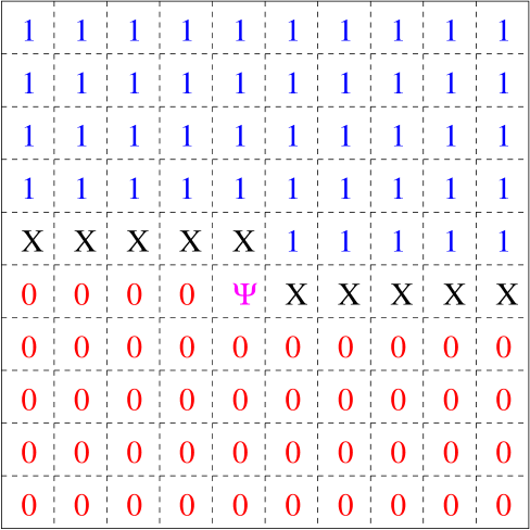
FIG. 1.: Integrating out sequentially, all finished sites are empty and out of range sites are filled. When integrating the site labeled $\psi$, only those sites labeled “X” are undetermined.

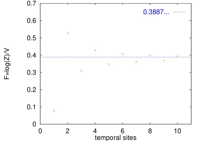
FIG. 2.: The free energy $F=\log(Z)/N_{i}N_{t}$ on an $N_{i}=50$ site chain as a function of the number of time slices $N_{t}$. The infinite volume solution is shown by the horizontal line.

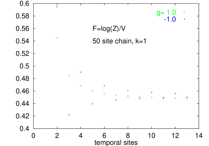
FIG. 3.: The free energy $F=\log(Z)/N_{i}N_{t}$ with a four fermion interaction as described in the text, plotted as a function of the number of time slices $N_{t}$. The chain has $N_{i}=50$ sites. Points are shown for $k=1$ and $g=\pm 1$.

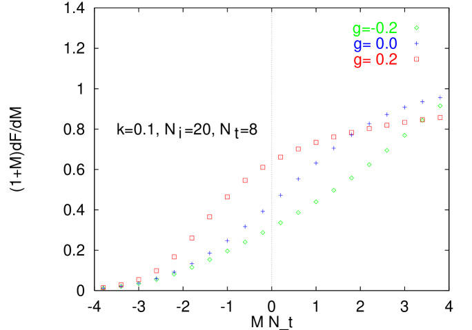
FIG. 4.: The occupancy of a 20 site chain as a function of the chemical potential scaled by the number of time slices. Note how the filling occurs earlier or later depending on the sign of the four fermion coupling. Here the spatial hopping parameter is taken as $K=0.1$

REFERENCES

- [1] F.A. Berezin, The method of second quantization, (Academic Press, NY, 1966).
- [2] I.M. Barbour and A.J. Bell, Nucl. Phys. B372, 385 (1992); I.M. Barbour, J.B. Kogut, and S.E. Morrison, Nucl. Phys. B (Proc. Suppl.) B53, 456 (1997).
- [3] Binder Physica 62 (1972) 508; T. de Neef and I.G. Enting, J. Phys. A10, (1977) 801; I.G. Enting, Aust. J. Phys. 31 (1978) 515; A.J. Guttmann and I.G. Enting, Nucl. Phys. B (Proc. Suppl.) 17 (1990) 328; G. Bhanot, M. Creutz, I. Horvath, J. Lacki, and J. Weckel, Phys. Rev. E49, 2445 (1994).
- [4] M. Creutz, Phys. Rev. B45, 4650 (1992).
- [5] M. Creutz, Phys. Rev. D35, 1460 (1987)
- [6] J. Hubbard, Proc. R. Soc. London A276, 283 (1963); A281, 401 (1964).
- [7] M. Creutz, M. Tytgat, C. Rebbi, S.-S.Xue, Physics Letters B402, 341-345 (1997).