TIFR/TH/98-23 June, 1998 hep-lat/9806034

Dimensional Reduction and Screening Masses
in Pure Gauge Theories at Finite Temperature

Saumen Datta and Sourendu Gupta

Department of Theoretical Physics,

Tata Institute of Fundamental Research,

Homi Bhabha Road, Mumbai 400005, India.

We studied screening masses in the equilibrium thermodynamics of $SU(2)$ and $SU(3)$ pure gauge theories on the lattice. At a temperature of $2T_{c}$ we found strong evidence for dimensional reduction in the non-perturbative spectrum of screening masses. Mass ratios in the high temperature $SU(3)$ theory are consistent with those in the pure gauge theory in three dimensions. At the first order $SU(3)$ phase transition we report the first measurement of the true scalar screening mass.

1 Introduction

The equilibrium thermodynamics of a gauge theory is studied in the non-perturbative domain by lattice simulations of the partition function. Much is now known about the phase transitions in $SU(2)$ and $SU(3)$ pure gauge theory and in QCD, including the order, the transition temperature, $T_{c}$, entropy density, pressure, specific and latent heats and other such quantities [1].

Also of interest are the screening masses at finite temperatures. These are defined in general by the exponential spatial falloff of the correlation of two static sources. A classification of all masses is provided by the transformation properties of the sources. For glueball-like screening masses, such a classification was performed in [2] where the first measurements of several of these masses were reported. Extensive lattice data is available on screening masses from meson and baryon-like sources [3], and on the correlation of Polyakov lines.

A gauge invariant transfer matrix formulation is easy to write for the lattice regularised theory. For thermal physics, it is convenient to think of the transfer matrix in a spatial direction. The free energy and other bulk thermodynamic quantities involve only the largest eigenvalue of the transfer matrix. Correlation functions and the screening masses involve the ratio of this largest eigenvalue with specific other eigenvalues depending on the transformation properties of the source. Thus, the full spectrum of screening masses contains much more information about the theory than bulk thermodynamics can provide.

A quantity of special interest is the Debye screening mass, $M_{D}$, whose inverse gives the screening length of static choromo-electric fields. In the quantum theory, this screening mass plays an important role in regulating some infra-red singularities. Lattice measurements have, in the past, concentrated on measuring a mass from the correlation of Polyakov loops, $M_{P}$. It was expected that when the gauge coupling becomes small, $M_{P}=2M_{D}$. Many years ago Nadkarni showed that the relation between $M_{D}$ and $M_{P}$ is far from being so simple [4]. Subsequent lattice work focussed on methods of computing $M_{D}$.

Reisz and collaborators [5, 6] wrote down a dimensionally reduced theory which could be used to define $M_{D}$ non-perturbatively. A recent paper [7] used the representations of the symmetries of the transfer matrix to write down operators whose correlations could be used to measure the Debye mass and gave a general parametrisation of the perturbative and non-perturbative terms for $M_{D}$. These parameters have since been determined in a lattice measurement of the Debye screening mass using a dimensionally reduced theory at very high temperatures [8].

A similar screening mass is required for the magnetic sector of the nonabelian gauge theory in the plasma, in order to get sensible results in the infrared. However, the magnetic mass is entirely non-perturbative in nature. It has been the object of many lattice studies [9, 10]. In fact, a recent work [10] tries to extract $M_{D}$ and $M_{m}$ from gauge fixed gluon propagators at finite temperature.

Many years ago Linde discovered [11] that the thermal perturbation expansion in non-Abelian gauge theories breaks down because the magnetic sector is not amenable to perturbative studies. A recent attempt to understand Linde’s problem in the region where the coupling $g\ll 1$ has invoked a sequence of dimensionally reduced effective theories [12]. At length scales of $1/gT$ dimensional reduction yields a three dimensional $SU(N)$ gauge theory coupled to an adjoint scalar field of mass $M_{D}\approx{\cal O}(gT)$. At longer scales, $1/g^{2}T$, the scalar field can be integrated out, and the leading terms in the effective theory correspond to a pure gauge theory in three dimensions. On the basis of this reduction it has been argued [12, 7] that a non-vanishing pole in magnetic gluon propagators is absent, and Linde’s problem is finessed by confinement in the three dimensional gauge theory.

In fact, dimensional reduction has often been used to explore finite temperature theories [13], and it has long been argued that the dimensionally reduced theory is confining. The spatial string tension is known to be non-vanishing for $T>T_{c}$ and scales as $T^{2}$ [14]. This, and other, lattice measurements reveal that the gauge coupling close to $T_{c}$ are too large to trust perturbation theory.

At temperatures of a few $T_{c}$, the coupling $g\geq 1$, and the length scales $1/T\approx 1/gT\approx 1/gT^{2}$, and hence cannot be decoupled. The construction of [12] is not applicable. However, the transfer matrix argument assures us that $M_{D}$ is only the smallest in a hierarchy of screening masses. We can then use the spectrum of the screening masses to explore the symmetries of the transfer matrix and check whether or not dimensional reduction works; and if it does, then what is the nature of the reduced theory.

Our major result is that the degeneracies of the spectrum of screening masses implies that the symmetry group of the spatial transfer matrix is that of two dimensional rotations— implying dimensional reduction for $T\approx 2T_{c}$. The measured non-perturbative spectrum is similar to that in 3-d pure gauge theory [15].

The symmetries of the transfer matrix, and the physical consequences are discussed in Section 2. The group theory presented in this section is central to the rest of this paper. The extraction of screening masses in $T>0$ four-dimensional $SU(3)$ and $SU(2)$ pure gauge theories take up the next two sections. These may be skipped by those readers who are not interested in the details of the lattice simulations. Section 5 contains a summary of our lattice results and presents our conclusions on the nature of the dimensionally reduced theory. Several technical details are relegated to appendices. Appendix A gives the loop operators used in our computations. In Appendix B, we examine the possibility of explaining the mass spectrum in terms of perturbative multigluon states. Noise reduction techniques for the lattice simulations and the algorithm for projecting on to the lowest state in every channel are described in Appendices C and D respectively.

2 Symmetries of the Transfer Matrix

2.1 Group chains

For the $T=0$ continuum Euclidean theory the symmetry of the transfer matrix is the direct product of the full rotation group $O(3)$ and the $Z_{2}$ groups generated by charge conjugation, $C$, and time reversal. Irreps of $O(3)$ are labelled by the angular momentum and parity, $J^{P}$, and of the full symmetry group by $J^{PC}$. For the lattice regularised theory, $O(3)$ breaks to the discrete subgroup of the symmetries of the cube, $O_{h}$. The consequent reduction of the irreps of $O(3)$ is well-known [16].

In the Euclidean formulation of the (continuum) equilibrium $T>0$ theory, the transfer matrix in one of the spatial directions is invariant under symmetries of the orthogonal slice. Such slices are three dimensional— two of which are spatial and one is the Euclidean time. The symmetry group is that of a cylinder, ${\cal C}=O(2)\times Z_{2}$. This $Z_{2}$ factor is generated by $\sigma_{z}\;:\;t\mapsto-t$. The non-Abelian group $O(2)$ contains the Abelian subgroup of rotations, $SO(2)$, and a 2-d parity, $\Pi\;:\;(x,y)\mapsto(x,-y)$. The 3-d parity $P=C(\pi)\sigma_{z}$, where $C(\pi)$ is the rotation by $\pi$ in $SO(2)$.

In the high temperature limit, the effective theory is expected to undergo dimensional reduction to a 3-d gauge theory. In such a theory, the transfer matrix must have the $O(2)$ symmetry of a 2-d slice. $O(2)$ has two one-dimensional irreps $0_{\pm}$ (the 2-d scalar and pseudo-scalar) and an infinite tower of two-dimensional irreps $M$. Under the reduction of $SO(3)$ to $O(2)$, the spin $J$ irrep breaks as—

$$J\;\to\;0_{\Pi(J)}+\sum_{M=1}^{J}M,\qquad{\rm where}\quad\Pi(J)=(-1)^{J}.$$ (2.1)

On the lattice the irreps of $\cal C$ break further into irreps of the automorphism group of a $z$-slice, the tetragonal group $D^{4}_{h}=D_{4}\times Z_{2}(P)$. For the three dimensional lattice theory, the automorphism group of the 2-d slice is $C^{4}_{v}$, which is isomorphic to $D_{4}$. A recent work on 3-d glueballs used this classification of the states [15].

This pattern of symmetry breaking is summarised by

$$\matrix{O(3)=SO(3)\times Z_{2}(P)&\longrightarrow&O_{h}=O\times Z_{2}(P)\cr\bigg{\downarrow}&&\bigg{\downarrow}\cr{\cal C}=O(2)\times Z_{2}(\sigma_{z})&\longrightarrow&D^{4}_{h}=D^{4}\times Z_{2}(P)\cr\bigg{\downarrow}&&\bigg{\downarrow}\cr O(2)&\longrightarrow&C^{4}_{v}\cr}$$ (2.2)

Four of the $Z_{2}$ factor groups are identical, and generated by the 3-d parity $P$. $O(2)$ and $C^{4}_{v}$ contain the 2-d parity $\Pi$.

2.2 Point group representations

In this paper we use the notation of [17] for the crystallographic point groups and their irreducible representations (irreps). This subsection contains a discussion of the irreducible representations of the lattice symmetries.

The group $D_{4}$ is generated by eight elements in five conjugacy classes— the identity ($E$), rotations of $\pm\pi/2$ around the $z$-axis ($C_{4}$), rotations of $\pi$ around the $z$-axis ($C_{4}^{2}$), around the $x$ or $y$-axes ($C_{2}$) and around the directions $x\pm y$ ($C_{2}^{\prime}=C_{4}C_{2}$). The five irreps are called $A_{1}$, $A_{2}$, $B_{1}$, $B_{2}$ and $E$. The first four are one-dimensional and the last two-dimensional. The 10 irreps of $D^{4}_{h}$ are obtained by adjoining the character of $P$ to the irreps of $D_{4}$. Under the reduction of $O_{h}$ to $D^{4}_{h}$, the irreps break up as—

$$A_{1}^{P}\; \to \;A_{1}^{P},\;\;\qquad\qquad A_{2}^{P}\;\to\;B_{1}^{P},$$ (2.3)

$$T_{1}^{P}\; \to \;A_{2}^{P}+E^{P},\qquad T_{2}^{P}\;\to\;B_{2}^{P}+E^{P},$$ (2.4)

$$E^{P}\; \to \;A_{1}^{P}+B_{1}^{P}.$$ (2.5)

The notation $A_{1,2}^{\pm}$ is potentially confusing since these irreps can belong to both $O_{h}$ and $D^{4}_{h}$. A similar confusion can also be caused by the notation $E$, which stands for the two-dimensional irrep of any group. In the rest of this paper we will mention the group involved whenever we mention one of these irreps.

In the dimensionally reduced theory, the lattice symmetry group is $C^{4}_{v}\simeq D_{4}$. Instead of calling the irreps by the names of the $D_{4}$ irreps, we denote them by the symbols $A^{+}$, $A^{-}$, $B^{+}$, $B^{-}$ and $E$ respectively. The first four are one-dimensional irreps, and the sign which indexes them is the character of the 2-d parity $\Pi$ in the irrep. The breaking of $D^{4}_{h}$ irreps to $C^{4}_{v}$ is as—

$$A_{1}^{+},A_{2}^{-}\; \to \;A^{+},\qquad A_{1}^{-},A_{2}^{+}\;\to\;A^{-},$$ (2.6)

$$B_{1}^{+},B_{2}^{-}\; \to \;B^{+},\qquad B_{1}^{-},B_{2}^{+}\;\to\;B^{-},$$ (2.7)

$$E^{P}\;\; \to \;E.\qquad$$ (2.8)

Our nomenclature for the irreps of $D^{4}_{h}$ is designed to be a mnemonic for the breaking of the $O_{h}$ irreps (eq. 2.5), but not for the breaking of $D^{4}_{h}$ to $C^{4}_{v}$ (eq. 2.8). On the other hand, the naming convention followed in [2, 7] simplifies the latter at the expense of the former, since it proceeds from the isomorphism $D^{4}_{h}\simeq C^{4}_{v}\times Z_{2}(\sigma_{z})$. To make contact with the notation used elsewhere, note that $P$ in [7] corresponds to our 2-d parity $\Pi$ and $R_{\bar{z}}$ to the character of the operator $\sigma_{z}$, which is called $P$ in [2].

The $O(2)$ irreps break to $C^{4}_{v}$ as follows—

$$0_{+}\; \to \;A^{+},\qquad\qquad{\rm and}\qquad 0_{-}\;\to\;A^{-},$$ (2.9)

$$M\; \to \;\cases{E&$(M={\rm odd}),\qquad$\cr B^{+}+B^{-}&$(M=2{\rm\ mod\ }4),$\cr A^{+}+A^{-}&$(M=0{\rm\ mod\ }4).$\cr}$$ (2.10)

The $A^{+}$ corresponds to the scalar and the $A^{-}$ to the pseudo-scalar irrep of $O(2)$.

States or operators also carry a label $C=\pm 1$ for the charge conjugation symmetry. The charge conjugation operator reverses the direction of traversal of a loop, and hence takes the trace into its complex conjugate. $C=1$ states correspond to real parts of loops and $C=-1$ states to imaginary parts. For gauge groups with only real representations, such as $SU(2)$, there are no $C=-1$ states. The construction of irreps of $D^{4}_{h}$ from loops is given in Appendix A.

Figure 1: Possible temperature dependence of the lowest screening masses in some channels. Dimensional reduction at high temperatures is signalled by a pattern of approximate degeneracies characteristic of $C^{4}_{v}$ symmetry.

In finite temperature lattice simulations, the symmetry group of the transfer matrix is always $D^{4}_{h}$. However, at low temperatures, we should expect to see an effective symmetry group $O_{h}$. At the other end of the temperature scale, if dimensional reduction is to be a good approximation, we should see an approximate $C^{4}_{v}$ symmetry. A guess at the temperature dependence of the screening masses is shown in Figure 1. If the lattice is big enough, and the lattice spacing is sufficiently small, then we should see the more extended degeneracy of $O(2)$. In this case the $A^{+}$ and $A^{-}$ of $C^{4}_{v}$ will be non-degenerate, since they correspond to different irreps of $O(2)$, but the $B^{+}$ and $B^{-}$ will become degenerate, since they correspond to one irrep of $O(2)$. Differences between first and second order phase transitions should be visible in the $A_{1}^{++}$ channel near $T_{c}$.

3 $SU(3)$ Pure Gauge Theory

We have simulated the $SU(3)$ pure gauge theory with Wilson action at three temperatures. With $N_{\tau}=4$ the critical coupling is $\beta_{c}(N_{\tau}=4)\;=\;5.692$ [18, 19]. We have performed a simulation at $T\approx T_{c}$ with $\beta=5.7$. At $T=3T_{c}/2$ the coupling is $\beta_{c}(N_{\tau}=6)\approx 5.9$ [19], and for $T=2T_{c}$ we use the coupling $\beta_{c}(N_{\tau}=8)\approx 6.0$ [20].

The simulations were performed with a Cabbibo-Marinari pseudo heat-bath update, where each update acted on three separate $SU(2)$ subgroups by five Kennedy-Pendleton moves [21]. The class of loop operators measured is listed in Appendix A. Noise reduction involved a fuzzing procedure explained in Appendix C. For each irrep of the symmetry group, we projected the measured correlation function to the ground state by a variational technique explained in Appendix D. Successive measurements of correlation functions were separated by about one integrated auto-correlation time measured through the Polyakov loop.

One of the techniques for extracting screening masses from correlation functions in the long direction (with $N_{z}$ sites) is to solve the equation

$${\cosh\left[m(z+1/2)(N_{z}/2-z-1)\right]\over\cosh\left[m(z+1/2)(N_{z}/2-z)\right]}\;=\;{C(z+1)\over C(z)}$$ (3.1)

for the local mass, $m(z+1/2)$, given measurements of the correlation function $C(z+1)$ and $C(z)$. The assumption that the correlation function is described by a single mass is borne out if there is a range of $z$ for which the local mass is constant within errors. If there is such a plateau then we quote it as our estimate of the screening mass.

In addition we have performed fits to correlation functions in the form

$$C(z)\;=\;C(0)\left\{r{\cosh\left[\mu_{0}(N_{z}/2-z)\right]\over\cosh(\mu_{0}N_{z}/2)}+(1-r){\cosh\left[\mu_{1}(N_{z}/2-z)\right]\over\cosh(\mu_{1}N_{z}/2)}\right\},$$ (3.2)

where $r$, $\mu_{0}$ and $\mu_{1}$ are fit parameters with the constraint $\mu_{0}<\mu_{1}$. Local mass estimates were deemed acceptable if the fitted value of $\mu_{0}$ agreed with it. When the local masses were too noisy to show a plateau, we took $\mu_{0}$ as our estimate of the screening mass. The goodness of the variational projection to the ground state was checked by observing whether the fitted parameter $r$ was close to unity.

In minimising $\chi^{2}$ to perform the fits we took into account covariances of data [22]. Since we normalised the variational correlator at separation zero to unity, the error in this point is zero. However, the intrinsic variability in the zero distance correlator is then redistributed over all the points through the covariance. The maximum distance retained in the fit was always determined by the criterion that the correlation function at that distance should be more than 1-$\sigma$ from zero. The estimates and errors of every measurable were constructed through a jack-knife procedure.

3.1 $T=T_{c}$

Figure 2: $A_{1}^{++}$ correlation functions in $SU(3)$ at $\beta=5.7$ with $(0,1)$ variation. (a) Data and fits for the projection to the lowest mass (thermal $A_{1}^{++}$: dark circles, $T=0$ $A_{1}^{++}$: grey circles, $T=0$ $E^{++}$: white circles), (b) local masses compared to the 1-$\sigma$ band around the best fit, (c) data and fits to the projection on the second mass, and (d) local masses compared to the 1-$\sigma$ error band on the fitted physical $A_{1}^{++}$ mass.

Operator	$(0,1)$			$(0,2)$
	$\chi^{2}$	$r$	$\mu_{0}$	$\chi^{2}$	$r$	$\mu_{0}$
$\left.A_{1}^{++}\right|_{0}$	$5.7/6$	$0.71_{-0.05}^{+0.04}$	$0.27_{-0.02}^{+0.01}$	$6.3/6$	$0.74_{-0.05}^{+0.04}$	$0.27_{-0.02}^{+0.01}$
$\left.E^{++}\right|_{0}$	$2.6/6$	$0.68_{-0.07}^{+0.05}$	$0.23_{-0.02}^{+0.02}$	$2.0/6$	$0.71_{-0.07}^{+0.05}$	$0.23_{-0.02}^{+0.02}$
$\left.A_{1}^{++}\right|_{T}$	$10.5/6$	$0.81_{-0.04}^{+0.03}$	$0.26_{-0.01}^{+0.01}$	$10.9/6$	$0.83_{-0.04}^{+0.03}$	$0.26_{-0.01}^{+0.01}$
$\left.B_{1}^{++}\right|_{T}$			$1.23\pm 0.08$			$1.2\pm 0.1$

Table 1: Fitted masses in $SU(3)$ theory for $\beta=5.7$ on the $4\times 8^{2}\times 16$ lattice using 5000 configurations. Note that $r$ depends on the basis set of operators, but $\mu_{0}$ does not. For the $B_{1}^{++}$ operator, a plateau in the local masses is used for the estimate of the screening mass.

At $\beta=5.7$ we analysed configurations separated by 50 pseudo-heat-bath sweeps, discarding the first 20 configurations for thermalisation. Tunnelling between phases occurred every 600 sweeps on an average. The operators measured are listed in Appendix A. Analyses were performed in subspaces corresponding to the $O_{h}$ and $D^{4}_{h}$ irreps.

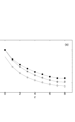
From the results in Table 1, it is clear that the lowest screening mass observed in the $\left.A_{1}^{++}\right|_{0}$ and $\left.E^{++}\right|_{0}$ sectors coincides with that obtained in the $\left.A_{1}^{++}\right|_{T}$ sector. This is also clear from Figure 2. In addition, the eigenvector of the variation over all operators was orthogonal (within errors) to the $\left.B_{1}^{++}\right|_{T}$ space and yielded the same mass as the $\left.A_{1}^{++}\right|_{T}$. In the critical region, therefore, the spectrum of screening masses is organised in irreps of $D^{4}_{h}$. In [2] it was found that the screening masses could be organised into irreps of $D^{4}_{h}$ at $3T_{c}/2$, but not at $T_{c}/2$. Our observation extends this to the picture presented in Figure 1.

It is interesting to note that the projection to the $A_{1}^{++}$ ground state, as measured by $r$, increases with the number of operators used. This is a generic feature of the variational method and clearly seen in Figure 2b. Another generic feature is visible in the same figure— the fitted mass is the same as the stable long-distance local mass. Also, because the fit uses all the data points, its error is slightly smaller than that of the local mass.

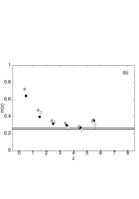
The lowest screening mass in the $\left.A_{1}^{++}\right|_{T}$ sector agrees with previous estimates of the mass from Polyakov line correlations [23]. This is the “tunnelling mass”, which goes to zero and decouples from the thermodynamics in the infinite volume limit. The mass in this channel, in the thermodynamic limit, should be finite, and on any finite lattice it would be the next-to-lowest $A_{1}^{++}$ mass. We attempted to estimate this “physical mass” by solving the variational problem for the second lowest eigenvalue. A common estimate of the mass is obtained from variation over all operators as well as only the $\left.A_{1}^{++}\right|_{T}$ operators. This indicates that the “physical mass” in the $\left.A_{1}^{++}\right|_{T}$ sector is genuinely the lowest screening mass. Local masses and fits agree (see Figure 2) and give a physical mass

$$am(A_{1}^{++})\;=\;0.86_{-0.10}^{+0.11},\qquad\qquad(N_{\tau}=4,\;\;\beta=5.7).$$ (3.3)

Such a physical mass has also been estimated before for two 3-state spin models in three dimensions. An $SU(3)$ spin model, obtainable from $SU(3)$ gauge theory in the strong coupling regime, had physical mass $0.71\pm 0.06$ [24] whereas the three state Potts model gave a mass of about $0.1$ [25]. The $A_{1}^{++}$ mass measured at $T=0$ at $\beta_{c}=5.7$ is $0.964\pm 0.012$ [26], giving

$${m(T_{c},A_{1}^{++})\over m(T=0,A_{1}^{++})}\;=\;0.89\pm 0.10.$$ (3.4)

In the scaling limit this ratio should be independent of $\beta_{c}$.

The $\left.B_{1}^{++}\right|_{T}$ operator is always a difference of loops. As a result the correlation function in this sector is much more noisy than in the $A_{1}^{++}$ sector. Nevertheless, we were able to follow the correlation function to distance 4, and obtain a plateau in the local masses. Our estimate of the screening mass, reported in Table 1, comes from the local mass, $m(5/2)$ for both $(0,1)$ and $(0,2)$ variation.

3.2 $T=3T_{c}/2$ and $2T_{c}$

We made runs on $4\times 8^{2}\times 16$ lattices at $\beta=5.9$ and 6.1, corresponding to $3T_{c}/2$ and $2T_{c}$ respectively. Since the integrated autocorrelation time for the Polyakov loop was estimated to be less than 10 sweeps, we analysed data separated by 10 sweeps after discarding the first 400 for thermalisation. 5000 configurations were generated at $3T_{c}/2$ and 10000 at $2T_{c}$. At $2T_{c}$ we made two further runs. One was on a larger, $4\times 12^{2}\times 16$ lattice, where we collected 5000 configurations separated by 10 sweeps, after discarding the first 400 sweeps. The second was on a shorter $4\times 8^{2}\times 12$ lattice, with exactly the same statistics. We did not see any tunnelling events at all in any of the four runs; from a hot start the system quickly relaxed into one of the $Z_{3}$ symmetric free-energy minima, and stayed there for the duration of the runs. Since measurements of autocorrelations of correlation functions showed that the integrated autocorrelation time did not exceed 1.5 measurements, these contributions to error estimates have been neglected in this section.

We made measurements of the operators listed in Appendix A. Each operator was replicated at five levels of fuzzing. In most channels we could follow the correlation functions out to distance 5 and found the $(0,z)$ variational ground state to be statistically well behaved even with $z$ as large as 3. The exceptions were the $B_{1}^{-+}$ and $B_{2}^{++}$ channels, which could be followed only to distance 3. As a result the variational ground state was stable only for $z=1$ and 2.

In each channel, the components of $|0;z\rangle_{T}$, the $(0,z)$ variational ground state at temperature $T$, give the overlaps of the ground state with each operator. We normalised $|0;z\rangle_{T}$ to unity in each jack-knife bin. We found that several components of this vector are numerically very stable from one jack-knife bin to another. The rest of the components fluctuate from bin to bin, and seem to fine tune the variational eigenvalue. The eigenvalue itself is far more stable than any of the eigenvectors.

We found that correlation functions at distance 1 differed qualitatively from the long distance correlation function in several respects, thus giving rise to certain systematics in the measurement of screening masses.

• The overlap $\langle 0;1|0;3\rangle_{2T_{c}}$ differed significantly from unity. For example, this overlap was $0.73\pm 0.02$ in the $A_{1}^{++}$ channel and $0.57\pm 0.05$ for the $A_{2}^{-+}$. On the other hand, the overlap $\langle 0;2|0;3\rangle_{2T_{c}}=0.90\pm 0.06$, consistent with unity, for $A_{1}^{++}$. Similar results were obtained at $3T_{c}/2$.

• There was a strong effect on local masses. With $(0,1)$ variation, we usually found no plateau in the local masses. With $(0,2)$ or $(0,3)$ variations a plateau was often visible.

• Fits to correlation functions also reflected this behaviour. No acceptable fit with one or two masses was found to the $(0,1)$ correlation function, whereas the $(0,3)$ correlator could be fitted with $r\simeq 1$.

In view of this, we quote results from the $(0,3)$ variational correlators in all channels except the $B_{1}^{-+}$ and $B_{2}^{++}$, for which we quote results from $(0,2)$ variation. All the screening masses we quote are obtained from local masses and verified by a fit. The exception is the $A_{2}^{-+}$ channel which turns out to be noisy. In this case the quoted result is the fitted mass.

The ground states in the $A_{1}^{-+}$, $A_{2}^{-+}$ and $B_{2}^{-+}$ channels are temperature independent within errors. This is not so in the $A_{1}^{++}$ and $B_{1}^{++}$ channels; the overlap of these two ground states at $3T_{c}/2$ and $2T_{c}$ are both $0.58\pm 0.02$. Interestingly, the masses are independent of the temperature.

$O(2)$	$D^{4}_{h}$	$3T_{c}/2$	$2T_{c}$
irreps	irreps	small	short	small	large
$0_{+}^{+}$	$A_{1}^{++}$	$0.64\pm 0.01$	$0.64\pm 0.01$	$0.65\pm 0.01$	$0.65\pm 0.02$
$0_{+}^{+}$	$A_{2}^{-+}$	$0.80\pm 0.02^{*}$	$0.61\pm 0.07^{*}$	$0.69\pm 0.04^{*}$	$0.68\pm 0.04^{*}$
$0_{-}^{+}$	$A_{1}^{-+}$	$1.58\pm 0.03$	$1.61\pm 0.06$	$1.58\pm 0.04$	$1.56\pm 0.04$
$2^{+}$	$B_{1}^{++}$	$1.22\pm 0.08$	$1.22\pm 0.05$	$1.2\pm 0.1$	$1.27\pm 0.06$
$2^{+}$	$B_{1}^{-+}$		$1.2\pm 0.1$	$1.34\pm 0.08$
$2^{+}$	$B_{2}^{++}$	$1.27\pm 0.07$	$1.3\pm 0.1$	$1.4\pm 0.1$	$1.3\pm 0.1$

Table 2: $SU(3)$ screening masses for $T>T_{c}$ on small ($4\times 8^{2}\times 16$), large ($4\times 12^{2}\times 16$) and short ($4\times 8^{2}\times 12$) lattices. The starred masses are obtained from two-mass fits, the rest from local masses. Data on $B_{1}^{-+}$ correlators was not collected in two cases.

Our results for the screening masses are collected in Table 2. The most interesting result is the near equality of the $A_{1}^{++}$ and $A_{2}^{-+}$ screening masses at $2T_{c}$. Similarly, the $B_{1}^{-+}$ and the $B_{2}^{++}$ masses are equal and also equal to the $B_{1}^{++}$ mass. Perturbation theory cannot be used to explain this pattern of degeneracies because the $P=1$ correlators require two gluon exchange, and the $P=-1$ correlation functions must have a minimum of four exchanged gluons.

Finite volume effects are under good control, as shown by the three separate runs on lattices of three sizes at $2T_{c}$. The study in [2] had shown that finite lattice spacing effects are also under control, by making two simulations at the same temperature but at two different lattice spacings. The values of $m/T$ in the $A_{1}^{++}$ and $A_{1}^{-+}$ channels were seen to be independent of the lattice spacing. We expect that this is true also of the screening masses in other channels, but would certainly welcome a direct measurement.

A comparison with zero temperature results is simple because $T=0$ measurements have been performed at both these couplings [26, 27, 28]. Using the results in [28] we find that at $\beta=5.9$

$${m(3T_{c}/2,A_{1}^{++})\over m(T=0,A_{1}^{++})}\;=\;0.78\pm 0.05,\qquad{m(3T_{c}/2,B_{1}^{++})\over m(T=0,E^{++})}\;=\;0.88\pm 0.09.$$ (3.5)

Moreover, at $\beta=6.0$ we find

$${m(2T_{c},A_{1}^{++})\over m(T=0,A_{1}^{++})}\;=\;0.90\pm 0.05,\qquad{m(2T_{c},B_{1}^{++})\over m(T=0,E^{++})}\;=\;1.12\pm 0.06.$$ (3.6)

These comparisons are made between channels at $T=0$ which overlap the corresponding channel at $T>0$. Although at this larger temperature the $T=0$ $A_{1}^{++}$ mass is nearly equal to the thermal $A_{1}^{++}$ screening mass, the state is completely different. The eigenvector of the variational problem has equal overlaps with the $T=0$ $A_{1}^{++}$ and $E^{++}$ states. It is clear that the physics observed here is completely different from the $T=0$ physics.

4 $SU(2)$ Pure Gauge Theory

The $SU(2)$ pure gauge theory with Wilson action was simulated at three temperatures. With $N_{\tau}=4$ the critical coupling is [29] $\beta_{c}(N_{\tau}=4)\;=\;2.2998$. We performed two simulations close to $T_{c}$— one with $\beta=2.30$, and another at $\beta=2.25$. With the lattice size we used, this other coupling is still within the critical region, as indicated by the Polyakov loop susceptibility [29]. We also performed simulations at $T=2T_{c}$ with $\beta_{c}(N_{\tau}=8)=2.51$ and at $T=4T_{c}$ with $\beta_{c}(N_{\tau}=16)=2.74$ [30].

These simulations were performed with an over-relaxation [31] and a Kennedy-Pendleton heat-bath algorithm [21]. The class of loop operators measured is listed in Appendix A. Each measurement of correlation functions was separated by about one integrated auto-correlation time measured through the Polyakov loop. The procedure for the analysis was identical to that for $SU(3)$.

4.1 $T\approx T_{c}$

$\beta$	Operator	$(0,1)$			$(0,2)$
		range	$\chi^{2}$	$\mu_{0}$	range	$\chi^{2}$	$\mu_{0}$
2.25	$\left.A_{1}^{+}\right|_{T(A)}$	[0:8]	0.32	$0.48^{+0.05}_{-0.06}$	[0:7]	0.11	$0.50^{+0.05}_{-0.06}$
	$\left.A_{1}^{+}\right|_{T(E)}$	[0:8]	0.87	$0.54^{+0.05}_{-0.07}$	[0:8]	0.26	$0.56^{+0.06}_{-0.06}$
	$\left.A_{1}^{+}\right|_{T}$	[0:8]	1.08	$0.53^{+0.05}_{-0.05}$	[0:8]	1.16	$0.54^{+0.05}_{-0.05}$
	$\left.B_{1}^{+}\right|_{T(E)}$	[0:5]	0.08	$1.26^{+0.08}_{-0.08}$	[0:5]	0.16	$1.11^{+0.10}_{-0.10}$
2.30	$\left.A_{1}^{+}\right|_{T(A)}$	[0:8]	0.50	$0.31^{+0.01}_{-0.01}$	[0:8]	1.02	$0.32^{+0.01}_{-0.02}$
	$\left.A_{1}^{+}\right|_{T(E)}$	[0:8]	0.63	$0.30^{+0.01}_{-0.01}$	[0:8]	0.55	$0.30^{+0.01}_{-0.01}$
	$\left.A_{1}^{+}\right|_{T}$	[0:8]	0.40	$0.30^{+0.01}_{-0.01}$	[0:8]	0.36	$0.30^{+0.01}_{-0.01}$
	$\left.B_{1}^{+}\right|_{T(E)}$	[0:5]	0.50	$1.10^{+0.04}_{-0.04}$	[0:5]	0.60	$1.09^{+0.04}_{-0.04}$

Table 3: Screening masses in the $SU(2)$ theory near $T_{c}$.

Figure 3: Correlation functions in $SU(2)$ at $\beta=2.3$ with $(0,1)$ variation. (a) Data and fits for the thermal $A_{1}^{+}$ correlator, (b) $A_{1}^{+}$ local masses compared to the 1-$\sigma$ band around the best fit, (c) data and fits to the $B_{1}^{+}$ correlator, and (d) $B_{1}^{+}$ local masses compared to the 1-$\sigma$ error band on the fit.

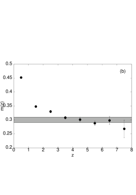
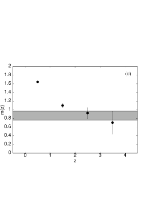
For $\beta=2.30$, we took one measurement on a $4\times 12^{2}\times 16$ lattice every 50 heatbath sweeps, and worked with $10000$ measurements after discarding the first 5000 sweeps for thermalisation. The set of operators measured is given in Appendix A. Our results for masses are presented in Table 3 and the correlation functions and masses are displayed in Figure 3.

The $\left.A_{1}^{+}\right|_{T}$ masses coming from the $O_{h}$ irreps $A_{1}^{+}$ and $E^{+}$ turn out to be identical. Note also that the parameter $r$ is rather large, indicating a successful projection onto the ground state. The $A_{1}^{+}$ mass is significantly smaller than the $T=0$ mass at the same coupling, $1.22\pm 0.03$ [32].

The $B_{1}^{+}$ correlator is significantly more noisy. However the correlation could be followed out to distance five. The mass estimate is fairly stable, and the overlap with the ground state is rather good. This screening mass is significantly higher than the $\left.A_{1}^{+}\right|_{T}$ screening mass, and much smaller than $m(T=0,E^{+})=1.94\pm 0.08$ [32], from which it comes.

At $\beta=2.25$ we took $10000$ measurements separated by 50 sweeps after discarding the first 5000 sweeps. Our fits indicate that the two screening masses for $\left.A_{1}^{+}\right|_{T}$, those from the $O_{h}$ irreps $A_{1}^{+}$ and $E^{+}$ are almost degenerate at this point, although the common mass is larger than that measured at $\beta=2.30$. The $\left.B_{1}^{+}\right|_{T}$ correlator was noisier, but good enough to yield a dependable measurement of the mass. This screening mass is clearly split from the $\left.A_{1}^{+}\right|_{T}$ mass coming from the same $O_{h}$ irrep $E^{+}$. Our results are summarised in Table 3, and are in accord with the expectation in Figure 1.

4.2 $T=2T_{c}$ and $4T_{c}$

We performed runs with $4\times 8^{2}\times 16$ and $4\times 12^{2}\times 16$ lattices at $\beta=2.51$ ($2T_{c}$) and $\beta=2.74$ ($4T_{c}$). Three to five over-relaxation sweeps were followed by one heat-bath sweep. Since autocorrelation times of Polyakov loops and plaquettes were seen to be less than three such composite steps, we performed a measurement on every fifth composite step. In all these runs, the system quickly relaxed into one of the $Z_{2}$ symmetric minima of the free energy and stayed there through the duration of the run.

As explained in Appendix A, we measured two sets of operators. The larger set, A, included all the operators in the smaller set, B. The marginal improvement in the measurement of screening masses did not compensate for the longer CPU time spent in constructing the extra operators. On the smaller lattice we measured only the set A. At $2T_{c}$ we made 10000 measurements on the small lattice and 10000 measurements of the operator set B on the larger lattice. At $4T_{c}$ we took 5000 measurements on the small lattice, 20000 of the operator set B and 10000 of the operator set A on the large lattice.

In the best cases we could follow the correlation function out to distance 5, and the local mass $m(3/2)$ already belonged to a plateau. The $B_{1}^{-}$ and $B_{2}^{+}$ channels were noisy, and we could follow the correlator only to distance 3. For these two channels as well, we quote $m(3/2)$ as our estimate of the local mass. The $A_{2}^{-}$ channel was more noisy than for the $SU(3)$ theory. We were unable to make any measurement in this channel. Unlike the behaviour noticed for $SU(3)$, the analysis from $(0,1)$ variation gave results in agreement with $(0,2)$ variation. Hence we report our analysis from $(0,1)$ variation.

$D^{4}_{h}$	$2T_{c}$		$4T_{c}$
irrep	small A	large B	small A	large A	large B
$A_{1}^{+}$	$0.71\pm 0.05$	$0.69\pm 0.04$	$0.74\pm 0.07$	$0.73\pm 0.05$	$0.73\pm 0.05$
$A_{1}^{-}$	$1.14\pm 0.02$	$1.02\pm 0.02$	$1.10\pm 0.05$	$0.87\pm 0.04$	$0.88\pm 0.04$
$B_{1}^{+}$	$1.18\pm 0.03$	$1.62\pm 0.06$	$0.69\pm 0.02^{*}$	$1.08\pm 0.06$	$1.10\pm 0.06$
$B_{1}^{-}$	$1.9\pm 0.2$	$1.8\pm 0.1$	$1.8\pm 0.1$	$1.55\pm 0.06$	$1.54\pm 0.05$
$B_{2}^{+}$	$1.8\pm 0.1$	$1.75\pm 0.05$	$1.5\pm 0.2$	$1.60\pm 0.08$	$1.56\pm 0.04$

Table 4: Estimates of screening masses in the $SU(2)$ pure gauge theory from small ($4\times 8^{2}\times 16$) and large ($4\times 12^{2}\times 16$) lattices. The estimates are obtained from local masses, except the ones with a star. The latter are obtained from a fit.

The eigenvectors corresponding to the ground states are very stable in every channel other than the $B_{2}^{+}$, where it showed large bin-to-bin fluctuations. The eigenvalues were always more stable than the eigenvectors. The ground state obtained by the variational method changed little between $2T_{c}$ and $4T_{c}$ for the $A_{1}^{+}$, $A_{1}^{-}$ and $B_{1}^{-}$ states; the eigenvectors had an overlap consistent with unity. However, in the $B_{1}^{+}$ channel, this overlap was $0.70\pm 0.04$. The screening mass $m(B_{1}^{+})$ changes the most between $2T_{c}$ and $4T_{c}$.

Our results for the screening masses are summarized in Table 4. The measurement of the screening mass in the $A_{1}^{+}$ sector gives

$${m(T,A_{1}^{+})\over T}=\cases{2.8\pm 0.2&($T=2T_{c}$),\cr 2.9\pm 0.2&($T=4T_{c}$).\cr}$$ (4.1)

This is consistent with previous measurements from correlations of Polyakov loops, reported in [33, 6]. The near-equality of the $B_{1}^{-}$ and the $B_{2}^{+}$ screening masses are characteristic of a dimensionally reduced theory, and cannot be explained in perturbation theory.

The major difference between the $SU(2)$ and $SU(3)$ theories seems to be in the volume dependence of various screening masses. The $A_{1}^{+}$ mass is the only one which seems to be volume independent. The $B_{1}^{+}$ screening mass increases with volume, and the rest decrease. A more extensive study is required to obtain the infinite volume limit of these masses. Only after this is done can we say more about the nature of the dimensionally reduced theory.

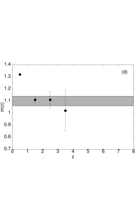
Our measurements of $m(T,A_{1}^{+})$ can be compared to the $T=0$ glueball masses measured at $\beta=2.5$ and $2.6$ [32]. Interpolation gives $m(T=0,A_{1}^{+})=0.70\pm 0.03$ for $\beta=2.51$. The mass ratio

$${m(2T_{c},A_{1}^{+})\over m(T=0,A_{1}^{+})}=0.99\pm 0.07,$$ (4.2)

is close to unity. Thermal effects are seen in the ground state— the $A_{1}^{+}$ eigenvector has a large projection on both the $T=0$ $A_{1}^{+}$ and $E^{+}$ channels. Glueball masses at $\beta=2.74$ for $T=0$ can be obtained by interpolating between the measurements at $\beta=2.7$ [34] and $\beta=2.85$ [35]. We estimate $m(T=0,A_{1}^{+})=0.35\pm 0.03$. Then

$${m(4T_{c},A_{1}^{+})\over m(T=0,A_{1}^{+})}=2.1\pm 0.2,$$ (4.3)

indicating a large thermal shift. This shows that the physics of screening masses is quite different from that of $T=0$ glueball masses.

5 Summary

In this section we summarise the results of our lattice measurements and discuss the physics implied by it. We try to deduce some general features of the dimensionally reduced theory by comparing these results with what is known of three dimensional gauge theories.

First we gather together our conclusions. We have found that for $T\geq T_{c}$ the spectrum of screening masses is completely consistent with a cylindrical symmetry of the spatial transfer matrix ($D^{4}_{h}$ on the lattice). At temperatures of $T_{c}$ and above, there is no remnant of the $T=0$ $O(3)$ rotational symmetry. The scalar representation of the cylinder group ($A_{1}^{++}$ on the lattice) gives the lowest screening mass at all temperatures in both $SU(2)$ and $SU(3)$ theories.

Near $T_{c}$ this lowest screening mass is very small. Since the $SU(2)$ gauge theory undergoes a second order deconfining transition, it is expected that this screening mass should be precisely zero on infinite volume systems. The small non-zero value we observe can be ascribed to finite-size effects.

The $SU(3)$ gauge theory has a first order deconfining transition. Finite-sized systems near a first order phase transition show a small screening mass, which vanishes in the infinite volume limit, and is related to tunnelings, and hence the surface tension [36], between the phases which coexist at a first order transition. Previous measurements [23] had seen only this mass. A technical point of interest to specialists is that our measurement of this mass yields results consistent with previous observations.

The important quantity for the study of screening masses is not this, but the finite screening mass— the “physical mass” in the $A_{1}^{++}$ channel for $SU(3)$ gauge theory. We have estimated it near $T_{c}$ for the first time.

$T$	$A_{1}^{++}$	$A_{1}^{-+}$	$B_{1}^{++}$	$B_{2}^{++}$
	$0_{+}^{+}$	$0_{-}^{+}$	$2^{+}$	$2^{+}$
$T_{c}$	3.4(4)	-	4.9(3)	-
$\frac{3}{2}T_{c}$	2.56(4)	6.3(1)	4.9(3)	5.1(3)
$2T_{c}$	2.60(4)	6.3(2)	4.8(1)	5.6(4)

Table 5: The ratio $m/T$ in various channels as a function of $T$ in the $SU(3)$ gauge theory. The $A_{1}^{++}$ screening mass shown near $T_{c}$ is the “physical mass”. The masses are labelled by the name of the 4-d lattice irrep (upper line) and the 3-d continuum irrep (lower line).

Our results for the screening masses are summarised in Table 5. As discussed in appendix B, the spectrum is not amenable to an understanding in terms of perturbative multigluon states, and gives nonperturbative information about the underlying effective theory.

Evidence for dimensional reduction at $2T_{c}$ comes from degeneracies in the spectrum of the transfer matrix. In the $SU(3)$ theory $m(A_{1}^{++})\simeq m(A_{1}^{-+})$, and $m(B_{1}^{-+})\simeq m(B_{2}^{++})\simeq m(B_{1}^{++})$. The first two sets of equalities are sufficient to argue for dimensional reduction of the lattice cutoff theory. The third equality implies $O(2)$ symmetry and hence allows us to make the stronger statement that the lattice artifacts are small. In the $SU(2)$ theory, although we have not eliminated lattice artifacts, dimensional reduction is shown by the relation $m(B_{2}^{+})\simeq m(B_{1}^{-})$.

Now we turn to possible interpretations of our detailed observations. The numerical values of the screening masses we have observed constrain the form of the three dimensional effective theory that describes equilibrium 4-d thermal gauge theories. In the scaling region of 3-d $SU(N)$ pure gauge theories, the glueball mass ratios

$${m(A^{++})\over m(B^{++})}\;=\;0.60,\qquad{m(B^{++})\over m(A^{-+})}\;=\;0.78,$$ (5.1)

are almost independent of $N$ for gauge groups $SU(N)$ [15]. Our measurements at $2T_{c}$ in the $SU(3)$ theory give

$${m(A^{++})\over m(B^{++})}\;=\;0.54\pm 0.02,\qquad{m(B^{++})\over m(A^{-+})}\;=\;0.76\pm 0.02.$$ (5.2)

From the spectrum it seems likely that the dimensionally reduced theory corresponding to the finite temperature $SU(3)$ theory may be a 3-d pure gauge theory.

One final observation— the $A_{1}^{+}$ mass in the $SU(2)$ theory agrees with many other measurements (performed through Polyakov loop correlations), and is expected to be independent of the lattice spacing. It is also seen to be independent of the lattice volume. In addition, it agrees numerically with the $A_{1}^{++}$ screening mass observed in the $SU(3)$ theory. It would be interesting to study whether the infinite volume limit of the other screening masses in both these theories show a similar agreement.

We will report on several technical points in future. A study of finite lattice spacing effects is under way. We are also performing a more extensive study of finite volume effects. We have not studied the two-dimensional irreps, $E$, of $D^{4}_{h}$, but expect that the screening masses in these channels would add to our understanding of this problem.

We would like to thank Rajiv Gavai for discussions.

Appendix A Loop Operators

We specify a loop with the notation $U_{i}(\mu,\nu,\lambda,\cdots)$. This denotes a product of link matrices starting with $U_{\mu}(i)$ and proceeding along the links in the directions $\nu$, $\lambda$, etc. The loops used in this work are drawn from the set—

$$P^{4}\;=\; {\rm Re\ Tr\ }U_{i}(\mu,\nu,-\mu,-\nu),\qquad\qquad\qquad$$

$$P^{6}\;=\; {\rm Re\ Tr\ }U_{i}(\mu,\mu,\nu,-\mu,-\mu,-\nu),\qquad\quad$$

$$T^{6}\;=\; {\rm Re\ Tr\ }U_{i}(\mu,\nu,\rho,-\mu,-\nu,-\rho),\qquad\quad$$

$$B^{6}\;=\; {\rm Re\ Tr\ }U_{i}(\mu,\nu,-\mu,\rho,-\nu,-\rho),\qquad\quad$$

$$O^{8}_{2}\;=\; {\rm Re\ Tr\ }U_{i}(\mu,\mu,\nu,\rho,-\mu,-\mu,-\rho,-\nu),$$

$$O^{8}_{3}\;=\; {\rm Re\ Tr\ }U_{i}(\mu,\mu,\nu,-\mu,\nu,-\mu,-\nu,-\nu),$$

$$O^{8}_{4}\;=\; {\rm Re\ Tr\ }U_{i}(\mu,\mu,\nu,-\mu,\rho,-\mu,-\rho,-\nu),$$ (A.1)

$$O^{8}_{5}\;=\; {\rm Re\ Tr\ }U_{i}(\mu,\mu,\nu,-\mu,\rho,-\nu,-\mu,-\rho),$$

$$O^{8}_{7}\;=\; {\rm Re\ Tr\ }U_{i}(\mu,\mu,\nu,\rho,-\nu,-\mu,-\mu,-\rho),$$

$$O^{8}_{14}\;=\; {\rm Re\ Tr\ }U_{i}(\mu,\nu,-\mu,-\nu,-\mu,\rho,\mu,-\rho),$$

$$O^{8}_{16}\;=\; {\rm Re\ Tr\ }U_{i}(\mu,\nu,-\mu,-\nu,-\rho,-\nu,\rho,\nu),$$

$$O^{8}_{17}\;=\; {\rm Re\ Tr\ }U_{i}(\mu,\nu,-\mu,-\nu,-\rho,\nu,\rho,-\nu),$$

$$O^{8}_{18}\;=\; {\rm Re\ Tr\ }U_{i}(\mu,\mu,\nu,-\mu,\rho,-\mu,-\nu,-\rho).$$

Our convention for naming these loops follows that of [16]. The plaquette ($P^{4}$), 6-link planar ($P^{6}$), twisted ($T^{6}$) and bent ($B^{6}$) loops, and the 8-link loop $O^{8}_{14}$ were considered in detail earlier [2]. We have also used the double traversal of some of these loops—

$$O^{2}\;=\;{\rm Re\ Tr\ }U_{i}U_{i},\qquad{\rm where}\qquad O\;=\;{\rm Re\ Tr\ }U_{i},$$ (A.2)

where $U_{i}$ is the $SU(N)$ matrix corresponding to a loop. The representation content of such pairs $O$ and $O^{2}$ are identical.

The irreps of the symmetry group can be constructed by acting on any loop by the projection operators of the group. For $D^{4}_{h}$ we use the operators

$$A_{1}^{\pm}\;= \;(E+C_{4})(E+C_{4}^{2})(E+C_{2})(E\pm P),$$

$$A_{2}^{\pm}\;= \;(E+C_{4})(E+C_{4}^{2})(E-C_{2})(E\pm P),$$

$$B_{1}^{\pm}\;= \;(E-C_{4})(E+C_{4}^{2})(E+C_{2})(E\pm P),$$ (A.3)

$$B_{2}^{\pm}\;= \;(E-C_{4})(E+C_{4}^{2})(E-C_{2})(E\pm P).$$

We have not used the remaining four projectors, which are the two independent sets each of $E^{+}$ and $E^{-}$ projectors that can be obtained by changing the sign of $C_{4}^{2}$ in the above formulæ. The irrep content of the loops in eq. (A) can simply be obtained using these projectors in a small Mathematica program.

In the $SU(3)$ measurements we used the following set of operators—

$$A_{1}^{++}\quad$$ (2) , (2) , (3) , (3) , (1) , (1) , (1) ,

(3) , (3)

(1) , (1) , (3) , (3)

(1) , (1) , (1) , (1) , (1) , (3) , (3)

(1) , (1) , (3) , (3) , (1) , (1) ,

(3) , (3)

(1) , (1) , (3) , (3)

(1) , (1) , (3) , (3)

For the simulation near $T_{c}$ only the plaquette and 6-link planar loops were used.

For the $SU(2)$ measurements a bigger set of operators was used—

$$A_{1}^{+}\quad$$ (2) , (3) , (2) , (1) , (2) , (2) , (3) ,

(2) , (3) , (2) , (2) , (2) , (3)

(3) , (2) , (2) , (2) , (3)

(3) , (1) , (1) , (1) , (1) ,(3)

(1) , (1) , (1) , (3) , (1) , (2) , (1) ,

(1) , (1) , (3)

(1) , (3) , (1) , (1) , (1) , (3) , (1) ,

(3) , (1) , (1) , (1) , (3)

(3) , (1) , (1) , (1) , (3)

(1) , (1) , (1) , (1) , (3) , (2) , (1) ,

(2) , (2) , (1) , (3)

(1) , (1) , (1) , (3) , (2) , (2) , (2) ,

(2) , (1) , (3)

along with the double traversals of each of them. This full set is the SET A of Section 4.2. Set B contained only the operators $P^{4}$, $P^{6}$, $B^{6}$, $T^{6}$, $O^{8}_{4}$, $O^{8}_{14}$, $O^{8}_{16}$ and $O^{8}_{18}$. For the simulations near $T_{c}$ only the plaquette and the six-link loops were used.

Appendix B Multi-gluon States

The simplest way of understanding the screening masses in the high temperature phase would be to accomodate it in a perturbative framework. Correlators of loops will then be dominated by suitable multigluon states, and the screening masses would give information on $M_{D}$ and $M_{m}$ [2]. Fortunately, such a hypothesis is open to a direct numerical test. In this appendix we show that the screening masses cannot be understood in perturbation theory.

$\bf k$	$A_{t}$	$A_{x},A_{y}$
(0,0,0)	$A_{2}^{-}$	$E^{-}$
(0,k,0)	$A_{2}^{-},B_{2}^{-},E^{+}$	$A_{1}^{+},B_{1}^{+},E^{-}$
(k,0,0)	$A_{1}^{+},A_{2}^{-}$	$E^{+},E^{-}$
(0,k,k)	$A_{2}^{-},B_{1}^{-},E^{+}$	$A_{1}^{+},A_{2}^{+},B_{1}^{+},B_{2}^{+},2E^{-}$
(0,k,k’)	$A_{1}^{-},A_{2}^{-},B_{1}^{-},B_{2}^{-},2E^{+}$	$A_{1}^{+},A_{2}^{+},B_{1}^{+},B_{2}^{+},2E^{-}$
(k,k’,0)	$A_{1}^{+},A_{2}^{-},B_{1}^{+},B_{2}^{-},E^{+},E^{-}$	$A_{1}^{+},A_{2}^{-},B_{1}^{+},B_{2}^{-},E^{+},E^{-}$
(k,k’,k”)	$A_{1}^{\pm},A_{2}^{\pm},B_{1}^{\pm},B_{2}^{\pm},E^{\pm},E^{\pm}$	$A_{1}^{\pm},A_{2}^{\pm},B_{1}^{\pm},B_{2}^{\pm},E^{\pm},E^{\pm}$

Table 6: The $D^{4}_{h}$ representation content of gluon operators at various points, $\bf k$, of the Brillouin zone. The first component of $\bf k$ is $k_{0}$. Note that all these irreps come with $C=-1$.

We first classify the irreps of $D^{4}_{h}$ which can be obtained by specific multi-gluon exchanges. The gluons carry arbitrary momenta, and are classified by representations of the space group. We break these irreps of the space group under the point group. Then the allowed representations for colour singlet zero momentum correlators are obtained by combining the gluon representations by the Clebsch-Gordan series for the point group $D^{4}_{h}$ and applying appropriate exchange symmetries.

We begin by specifying the lattice analogue of gluon field operators in momentum space by the Fourier transform of a projection of link matrices onto the $SU(N)$ algebra—

$$A_{\mu}({\bf k})\;=\;i\sum_{\bf x}{\rm e}^{i{\bf k}\cdot{\bf x}}\bigl{[}U_{\mu}({\bf x})-U^{\dagger}_{\mu}({\bf x})-{\rm Im\,Tr}\,U_{\mu}({\bf x})\bigr{]}.$$ (B.1)

Here $\bf x$ takes values in a slice orthogonal to the $z$-direction, and $\bf k$ in the corresponding Brillouin zone. In general, the action of $D^{4}_{h}$ carries one $\bf k$ into another. The representations built over the orbit of $\bf k$ under the action of $D^{4}_{h}$ are usually large and reducible. The representation content of such gluon field operators is gauge independent, and is shown in Table 6.

$\bf k$	$G^{(2)}_{tt}$	$G^{(2)}_{tx},G^{(2)}_{ty}$	$G^{(2)}_{xx},G^{(2)}_{yy}$	$G^{(2)}_{xy}$
(0,0,0)	$A_{1}^{+}$	$E^{+}$	$A_{1}^{+},B_{1}^{+}$	$B_{2}^{+}$
(0,k,0)	$A_{1}^{+},B_{1}^{+}$	$E^{+}$	$A_{1}^{+},B_{1}^{+}$	$A_{2}^{+},B_{2}^{+}$
(k,0,0)	$A_{1}^{+}$	$E^{+}$	$A_{1}^{+},B_{1}^{+}$	$B_{2}^{+}$
(0,k,k)	$A_{1}^{+},B_{2}^{+}$	$2E^{+}$	$A_{1}^{+},A_{2}^{+},$	$A_{1}^{+},B_{2}^{+}$
			$B_{1}^{+},B_{2}^{+}$
(0,k,k’)	$A_{1}^{+},A_{2}^{+},$	$2E^{+}$	$A_{1}^{+},A_{2}^{+},$	$A_{1}^{+},A_{2}^{+},$
	$B_{1}^{+},B_{2}^{+}$		$B_{1}^{+},B_{2}^{+}$	$B_{1}^{+},B_{2}^{+}$
(k,k’,0)	$A_{1}^{+},B_{1}^{+},E^{+}$	$A_{1}^{+},B_{1}^{+},E^{+}$	$A_{1}^{+},B_{1}^{+},E^{+}$	$A_{2}^{+},B_{2}^{+},E^{+}$
(k,k’,k”)	$A_{1}^{+},A_{2}^{+},B_{1}^{+},$	$A_{1}^{+},A_{2}^{+},B_{1}^{+},$	$A_{1}^{+},A_{2}^{+},B_{1}^{+},$	$A_{1}^{+},A_{2}^{+},B_{1}^{+},$
	$B_{2}^{+},E^{+}$	$B_{2}^{+},E^{+}$	$B_{2}^{+},E^{+}$	$B_{2}^{+},E^{+}$

Table 7: The irreps for symmetric colour singlet $C=1$ two-gluon states with total momentum zero are listed for the momentum, $\bf k$, of one of the gluon at various points in the Brillouin zone.

Gauge invariant $C=1$ states of zero momentum can be constructed as linear combinations of the composite operators

$$G^{(2)}_{\mu\nu}\;=\;Tr\,\bigl{[}A_{\mu}({\bf k})A_{\nu}(-{\bf k})\bigr{]},$$ (B.2)

where the trace is over $SU(N)$ generators. Correlators of such an operator will decay, in leading order, with the mass $E_{\mu}({\bf k})+E_{\nu}({\bf k})$, where $E_{0}=E_{D}$, $E_{1,2}=E_{m}$ and

$$\sinh^{2}(E_{D,m}({\bf k})/2)\;=\;\sinh^{2}(M_{D,m}/2)+\sum_{i=0}^{2}\sin^{2}(k_{i}/2).$$ (B.3)

The cyclic property of traces ensures that $G^{(2)}$ is symmetric under any operation that flips the polarisation indices and simultaneously changes the sign of $\bf k$. In addition, if we require that the state be symmetric under the exchange of the gluon fields, then only $P=1$ irreps are allowed. The representation content of these operators in all parts of the Brillouin zone is given in Table 7.

In order to obtain $P=-1$, $C=1$ irreps we have to go to combinations of four gluon field operators. Colour singlet gauge invariant correlators with $C=-1$ start with composite operators of three gluon fields.

The reduction of multi-gluon operators then tells us that

• For $C=1$, the lowest mass observed in any $P=1$ channel would be at most half of the lowest mass observed in any $P=-1$ channel, since the former are obtained by two-gluon exchange but the latter require at least four-gluon exchange.

• If $E_{m}({\bf 0})<E_{D}({\bf 0})$, then $m(A_{1}^{++})=m(B_{1}^{++})=m(B_{2}^{++})$.

• If $E_{D}({\bf 0})<E_{m}({\bf 0})<E_{D}({\bf K})$, for ${\bf K}=(0,2\pi/N_{x},0)$, then $m(B_{1}^{++})=m(B_{2}^{++})$ and the mass difference between the $A_{1}^{++}$ and $B_{1}^{++}$ states is $2[E_{m}({\bf 0})-E_{D}({\bf 0})]$. Here $N_{x}$ is the spatial size of the $z$-slice.

• If $E_{m}({\bf 0})>E_{D}({\bf K})$, then $m(B_{1}^{++})<m(B_{2}^{++})$ and the mass difference $m(B_{1}^{++})-m(A_{1}^{++})$ decreases with lattice size.

The first condition is clearly violated in the spectra we obtain for both $SU(2)$ and $SU(3)$ theories. At $2T_{c}$ in both the theories we found $m(B_{1}^{-+})\simeq m(B_{2}^{++})$. In addition, in the $SU(3)$ theory $m(A_{1}^{++})\simeq m(A_{2}^{-+})$. Both these observations violate the first condition. This is sufficient evidence for a failure of the interpretation of these masses as screening masses for perturbative multigluon states.

If we ignore this, and restrict ourselves to the $P=1$, $C=1$ states only, then one might be tempted to match the $SU(3)$ spectrum to the third condition above, since the mass difference $m(B_{1}^{++})-m(A_{1}^{++})$ is non-zero and independent of the lattice size. However, from eq. (B.3), the condition $M_{m}<E_{D}({\bf k})$ is satisfied for $N_{x}=8$ but not for $N_{x}=12$. Thus, none of the conditions above hold, and we conclude that the spectrum of screening masses cannot be given a perturbative interpretation of multigluon states, and indeed gives information about the nonperturbative spectrum of the effective theory. A similar statement has been made in ref. [37] in the context of the massgap obtained from Polyakov loop correlators at moderate temperatures, on the basis of the detailed decay patterns of the correlators seen in lattice studies.

Appendix C Improved Operators

Loop correlations are known to be very noisy. In order to increase the signal/background ratio, we used a hybrid of Teper’s doubled-link fuzzing procedure [38] and the smearing procedure adopted by the APE collaboration [39]. We define fuzzed links at level $l+1$ recursively in terms of those at level $l$ by the equation

$${\rm max}\,{\rm tr}\left(M^{\dagger}_{i,\mu}U^{(l+1)}_{i,\mu}\right)\quad{\rm where}\quad M_{i,\mu}\;=\;U^{(l)}_{i,\mu}+\sum_{\nu\neq\mu,\hat{z}}U^{(l)}_{i,\nu}U^{(l)}_{i+\nu,\mu}U^{\dagger(l)}_{i+\mu,\nu},$$ (C.1)

$U^{(l+1)}$ are elements of $SU(N)$, and the links for $l=0$ are those generated by the Monte Carlo procedure. For general $SU(N)$, this maximisation is most easily accomplished using the “polar” decomposition of a general complex matrix to write

$$M\;=\;\omega U^{(l+1)}H,$$ (C.2)

where $\omega$ is a complex number of unit modulus, $H$ is hermitian and $U^{(l+1)}$ is special unitary. There is a discrete ambiguity in this decomposition, corresponding to the signs of the eigenvalues of $H$. When all the eigenvalues of $H$ are chosen to be positive, $U^{(l+1)}$ maximises the trace in eq. (C.1). For $SU(2)$ the algorithm is simpler since $H$ is a multiple of the identity. The projection then involves only a division of $M$ by the square root of its determinant.

In a test run with $SU(3)$ at $\beta=5.7$ on a $4^{3}\times 12$ lattice, the procedure in eq. (C.1) was found to perform better than doubled-link fuzzing. Since the latter technique is known to work well on larger lattices, we conclude that the problem is due to the fact that with small lattices, only a small number of doubled-link fuzzing steps is possible. Presumably on larger lattices, where more fuzzing levels can be reached, equally good results can be obtained with either fuzzing technique. For the $SU(3)$ theory we worked with eq. (C.1) and $l\leq 4$.

For $SU(2)$, since we use a lattice which has 12 spatial sites, upto three levels of doubled-link fuzzing can be performed for the spatial links. For finite temperature problems it is perfectly all right if the number of fuzzing steps in the time direction is different from that in other directions. We perform only one doubled-link fuzzing in the time direction. We checked that using three levels of doubled-link fuzzing gave a better projection than seven steps of (C.1), and therefore used the former, for our runs near $T_{c}$. For our runs at $2T_{c}$ and $4T_{c}$, we experimented with a combination of doubled-link fuzzing and (C.1); using a combination of one doubled-link fuzzing followed by two steps of (C.1), the whole set being repeated once. Since this gave a slight improvement over three steps of doubled-link fuzzing, we used this technique at these higher temperatures. For our runs on the smaller lattice we used one doubled-link fuzzing followed by 4 steps of eq. (C.1).

Appendix D Variational Correlators

It is not known a priori which linear combination of loop operators acting on the vacuum generates the state with the lowest mass in a channel with given quantum numbers. However, such a state will give a correlation function which has the slowest possible decay with increasing separation. Given a basis set of loop operators, we can try to construct a linear combination which satisfies this property of slowest decay. This is the idea of a widely used variational technique [40]. Since we have found no discussion in the literature of a numerically stable algorithm for its implementation, we document such a method here.

We construct cross correlations between all the loop operators at our disposal to yield the (symmetric) matrix of correlations $C_{ij}(z)$. A combination of operators which has large projection to the ground state is obtained by solving the variational problem over $Y$—

$${\rm max}\left[{Y^{T}C(z_{1})Y\over Y^{T}C(z_{0})Y}\right]=\lambda(z_{0},z_{1}),\qquad(z_{0}<z_{1}).$$ (D.1)

If $C(z_{0})$ is positive definite, as guaranteed by the reflection positivity of the Wilson action, then this extremisation problem reduces to finding the maximum eigenvalue of the system—

$$C(z_{1})Y\;=\;\lambda(z_{0},z_{1})C(z_{0})Y.$$ (D.2)

With the corresponding eigenvector, we define the $(z_{0},z_{1})$ variational correlator

$$\widetilde{C}_{z_{0},z_{1}}(z)\;=\;Y^{T}C(z)Y.$$ (D.3)

We can utilise the freedom of normalising the eigenvector $Y$ to set the variational correlator to unity at separation $z=0$.

Reflection positivity of the action guarantees that $C(z_{0})$ is positive definite. It can be treated as a metric, and after appropriate scaling, the problem in eq. (D.1) can be phrased as the extremisation of a quadratic form over a sphere— leading to the usual matrix eigenvalue problem [41]. Algorithmically, this naive idea can be implemented by transforming both sides of eq. (D.2) to the basis where $C(z_{0})$ is diagonal, absorbing the diagonal elements into $Y$ by appropriate rescaling, and then solving the usual eigenvalue problem for this transformed $C(z_{1})$. However, if some of the eigenvalues of $C(z_{0})$ are small, then the extremum problem is ill-conditioned because the solution is sent off to infinity along the nearly flat directions.

With finite statistics the problem may be even worse. Due to statistical fluctuations, the measured correlation matrix may not be positive definite. It is then better to treat the problematic directions as exactly flat, since this discards the subset of the data which is most corrupted by noise. The solution is easily specified by going to the basis in which $C(z_{0})$ is diagonal and blocking the matrices into the form

$$C(z_{1})=\left(\matrix{C_{11}&C_{12}\cr C^{T}_{12}&C_{22}}\right),\qquad{\rm and}\qquad C(z_{0})=\left(\matrix{G&0\cr 0&0}\right),$$ (D.4)

where the eigenvalues, $e_{i}$, of $C(z_{0})$ which satisfy the cut condition

$$e_{i}\;<\;\epsilon e_{0}$$ (D.5)

have been set to zero. Here $e_{0}$ is the maximum eigenvalue of $C(z_{0})$. The diagonal sub-matrix $G$ is positive definite and has a condition number less than $1/\epsilon$. In this basis, eq. (D.1) is equivalent to the set of equations—

$$C_{11}Y_{1}+C_{12}Y_{2}=\lambda GY_{1}\qquad{\rm and}\qquad C^{T}_{12}Y_{1}+C_{22}Y_{2}=0.$$ (D.6)

Solving the latter for $Y_{2}$ and substituting into the former gives the eigenvalue problem—

$$\left[C_{11}-C_{12}C^{-1}_{22}C^{T}_{12}\right]Y_{1}=\lambda GY_{1},$$ (D.7)

which is well-defined and numerically well-conditioned as long as $C_{22}$ is invertible.

Notice, however, that eq. (D.2) is ill-conditioned only if both $C(z_{1})$ and $C(z_{0})$ have nearly flat directions; otherwise their roles may be interchanged by inverting eq. (D.1) and converting the maximum problem into that of finding a minimum. If this cannot be done, then we must take care of the case that $C_{22}$ is not invertible.

The $m\times n$ matrix $C^{T}_{12}$ is a map from $R^{n}$ to $R^{m}$ (i.e., $Y_{1}$ has $n$ real components and $Y_{2}$ has $m$). Its range is the subset of $R^{m}$ to which the whole of $R^{n}$ is mapped. If $C_{22}$ is singular, then its null-space is contained in the complement of the range of $C^{T}_{12}$. As a result, the second of eq. (D.6) can be solved by a left-multiplication by any matrix which coincides with the inverse of $C_{22}$ in the complement of its null-space (i.e., in the range of $C^{T}_{12}$). Therefore, in eq. (D.7) $C^{-1}_{22}$ can be replaced by a pseudo-inverse

$$C^{-1}_{22}=V^{T}\bar{\Lambda}^{-1}V\qquad{\rm where}\qquad C_{22}=V^{T}\Lambda V,$$ (D.8)

$V$ is an orthogonal matrix, $\Lambda$ is diagonal, and the small components of $\Lambda$ are set to zero in the pseudo-inverse $\bar{\Lambda}^{-1}$. With this definition of $C_{22}^{-1}$, the generalised eigenvalue problem is completely well-defined and eq. (D.7) may be solved by the naive algorithm described earlier.

Figure 4: Histogram of normalised eigenvalues of the $95\times 95$ correlation matrix at distance zero, $C(0)$ in the $A_{1}^{++}$ channel at $2T_{c}$ for the $SU(3)$ theory.

A very nice numerical illustration is provided by our data on the $95\times 95$ matrix of the $A_{1}^{++}$ correlation function at $2T_{c}$ for the $SU(3)$ gauge theory (section 3.2). The distribution of

$$x\;=\;\log_{10}\left({e_{0}\over|e_{i}|}\right),$$ (D.9)

is shown in Figure 4. The ten small eigenvalues clustered at the end of a huge spectral gap have both positive and negative signs, and are due to noise in the data. Because they are so well separated, the cut $\epsilon$ (in eq. D.5) can be chosen to have any value between $10^{-4}$ and $10^{-17}$. The results for eigenvalues and eigenvectors are stable in this whole range of choices. Somewhat smaller values, $\epsilon\approx 10^{-3}$, are also found to be acceptable and are in fact preferred for reasons of numerical stability of the linear algebra routines. Removing the cut destabilises the problem completely. The spectral distributions are similar in most channels for both $SU(2)$ and $SU(3)$ theories. In a few cases the spectral distribution is gapless but has a long tail. Even in such cases, $\epsilon\approx 10^{-3}$–$10^{-4}$ give stable results.

References

- [1] See for example, E. Laermann, Nucl. Phys., B (Proc. Suppl.), 63A-C (1998) 114, and references therein.
- [2] B. Grossman, S. Gupta, F. Karsch and U. Heller, Nucl. Phys., B 417 (1994) 289.
-
[3]
C. DeTar and J. Kogut, Phys. Rev. Lett., 59 (1987) 399;
Phys. Rev., D 36 (1987) 2828;
S. Gottlieb et al., Phys. Rev. Lett., 59 (1987) 1881;
A. Gocksch, P. Rossi and U. M. Heller, Phys. Lett., B 205 (1988) 334;
K. Born et al., Phys. Rev. Lett., 67 (1991) 302;
S. Gupta, Phys. Lett., B 288 (1992) 171;
C. Bernard et al., Phys. Rev. Lett., 68 (1992) 2125;
G. Boyd, S. Gupta and F. Karsch, Nucl. Phys., B 385 (1992) 481;
T. Hashimoto, T. Nakamura and I. O. Stamatescu, Nucl. Phys., B 400 (1993) 267. - [4] S. Nadkarni, Phys. Rev., D 33 (1986) 3738; and D 34 (1986) 3904.
[5]
A. Irbäck et al., Nucl. Phys., B 363 (1991) 34;
T. Reisz, Z. Phys., C 53 (1992) 169;
L. Kärkkäinen et al., Phys. Lett., B 282 (1992) 121;
L. Kärkkäinen, P. Lacock, B. Petersson and T. Reisz, Nucl. Phys., B 395 (1993) 733. - [6] P. LaCock and T. Reisz, Nucl. Phys., B (Proc. Suppl) 30 (1993) 307.
- [7] P. Arnold and L. G. Yaffe, Phys. Rev., D 52 (1995) 7208.
- [8] K. Kajantie et al., Phys. Rev. Lett., 79 (1997) 3130.
[9]
A. Billoire, G. Lazarides and Q. Shafi, Phys. Lett.,
B 103 (1981) 450;
T. A. DeGrand and D. Toussaint, Phys. Rev., D 25 (1982) 526;
G. Lazarides and S. Sarantakos, Phys. Rev., D 31 (1985) 389. - [10] U. M. Heller, F. Karsch and J. Rank, Phys. Rev., D 57 (1998) 1438.
- [11] A. D. Linde, Phys. Lett., B 96 (1980) 289.
[12]
E. Braaten, Phys. Rev. Lett., 74 (1995) 2164;
E. Braaten and A. Nieto, Phys. Rev. Lett., 74 (1995) 3530. -
[13]
P. Ginsparg, Nucl. Phys., B 170 (1980) 388;
T. Applequist and R. D. Pisarski, Phys. Rev., D 23 (1981) 2305;
K. Kajantie, K. Rummukainen and M. Shaposhnikov, Nucl. Phys., B 407 (1993) 356. -
[14]
G. Bali et al., Phys. Rev. Lett., 71 (1993) 3059;
L. Kärkkäinen et al., Phys. Lett., B 312 (1993) 173. - [15] M. Teper, preprint hep-lat/9804008.
- [16] B. Berg and A. Billoire, Nucl. Phys., B 221 (1983) 109.
- [17] M. Hamermesh, “Group Theory and its Applications to Physical Problems”, Addison-Wesley, Reading, Massachusetts, 1962.
- [18] M. Fukugita, M. Okawa and A. Ukawa, Nucl. Phys., B 337 (1990) 181.
- [19] Y. Iwasaki et al., Phys. Rev. Lett., 67 (1991) 3343, and Phys. Rev., D 46 (1992) 4657.
[20]
H. Ding and N. Christ, Phys. Rev. Lett., 60 (1988) 1367;
A. D. Kennedy, J. Kuti, S. Meyer and B. J. Pendleton, Phys. Rev. Lett., 54 (1985) 87;
S. A. Gottlieb et al., Phys. Rev. Lett., 55 (1985) 1958. - [21] A. D. Kennedy and B. J. Pendleton, Phys. Lett., B 156 (1985) 393.
- [22] S. Gottlieb et al., Phys. Rev., D 38 (1988) 2245.
- [23] F. R. Brown et al., Phys. Rev. Lett., 61 (1988) 2058. P. Bacilieri et al., Phys. Lett., B 220 (1989) 607.
- [24] S. Gupta et al., Nucl. Phys., B 329 (1990) 263.
- [25] R. V. Gavai, F. Karsch and B. Petersson, Nucl. Phys., B 322 (1989) 738.
- [26] H. Chen, J. Sexton, A. Vaccarino and D. Weingarten, Nucl. Phys. (Proc. Suppl.), B 34 (1994) 357.
- [27] Ph. de Forcrand, G. Schierholz, H, Schneider and M. Teper, Phys. Lett., B 152 (1985) 107.
- [28] C. Michael and M. Teper, Nucl. Phys., B 314 (1989) 347.
- [29] J. Engels, J. Fingberg and M. Weber, Nucl. Phys., B 332 (1990) 737.
- [30] J. Fingberg, U. Heller and F. Karsch, Nucl. Phys., B 392 (1993) 493.
- [31] M. Creutz, Phys. Rev. D 36 (1987) 515.
- [32] C. Michael and M. Teper, Phys. Lett., B 199 (1987) 95.
- [33] J. Engels, F. Karsch and H. Satz, Nucl. Phys., B 315 (1989) 419.
- [34] C. Michael and S. J. Perantonis, J. Phys., G 18 (1992) 1725.
- [35] S. P. Booth et al., Nucl. Phys., B 394 (1993) 509.
[36]
J. C. Neil and J. Zinn-Justin, Nucl. Phys., B 280 (1987) 355;
S. Gupta, Phys. Lett., B 325 (1994) 418. -
[37]
E. Braaten and A. Nieto, Phys. Rev. Lett., 74 (1995) 3530.
- [38] M. Teper, Phys. Lett., B 183 (1986) 345.
- [39] M. Albanese et al., Phys. Lett., B 192 (1987) 163.
- [40] M. Lüscher and U. Wolff, Nucl. Phys., B 339 (1990) 222.
[41]
J. H. Wilkinson, The Algebraic Eigenvalue Problem, 1965,
Clarendon Press, Oxford;
H. Rutishauser, Lectures on Numerical Mathematics, 1990, Birkhäuser, Boston, USA.