Four Fermion Models at Non-Zero Density

Abstract

I review the properties of the three-dimensional Gross-Neveu model formulated with non-zero chemical potential and temperature, focussing on results obtained by lattice Monte Carlo simulation.

1 INTRODUCTION

This talk concerns simulations of fermionic systems at non-zero density, which don’t suffer from the problems associated with gauge theories. To paraphrase the sub-title of the workshop, they could be described as “not-quite-so complex systems with a real action”; however, as I propose to show, the physics involved is still rich. The two theories I will discuss are referred to as “Gross-Neveu” models [1], and are described by the following Lagrangian densities:

$${\cal L}_{A} = \bar{\psi}_{i}({\partial\!\!\!/}\,+m)\psi_{i}-{g^{2}\over{2N_{f}}}(\bar{\psi}_{i}\psi_{i})^{2}$$ (1)

$${\cal L}_{B} = \bar{\psi}_{i}({\partial\!\!\!/}\,+m)\psi_{i}-{g^{2}\over{2N_{f}}}\left[(\bar{\psi}_{i}\psi_{i})^{2}-(\bar{\psi}_{i}\gamma_{5}\psi_{i})^{2}\right]$$ (2)

In each case the index $i$ runs over $N_{f}$ flavors of fermion, assumed to be four-component Dirac spinors. In the chiral limit $m\to 0$, symmetries akin to chiral symmetries can be identified:

$$A\;\;{\mbox{Z}}_{2}:\;\;\;\psi_{i}\mapsto\gamma_{5}\psi_{i}\;\;;\;\;\bar{\psi}_{i}\mapsto-\bar{\psi}_{i}\gamma_{5}\\$$ (3)

$$B\;\;{\mbox{U}(1)}:\;\;\;\psi_{i}\mapsto\exp(i\alpha\gamma_{5})\psi_{i}\;\;;\;\;\bar{\psi}_{i}\mapsto\bar{\psi}_{i}\exp(i\alpha\gamma_{5})$$ (4)

A version of the model with a global $\mbox{SU(2)}_{L}\otimes\mbox{SU(2)}_{R}$ symmetry can also be formulated.

I will focus on the case where the models (1,2) are formulated in three spacetime dimensions, where the following features hold:

1. For sufficiently strong coupling $g^{2}$ the models exhibit dynamical chiral symmetry breaking at zero temperature and density.

2. The spectrum of excitations contains both baryons and mesons, ie. the elementary fermions, and composite fermion – anti-fermion states.

3. The models have an interacting continuum limit.

4. For model $B$, whose chiral symmetry is continuous, the spectrum contains Goldstone modes.

5. When formulated on a lattice, the models have real Euclidean actions even for chemical potential $\mu\not=0$, and hence can be simulated by standard Monte Carlo techniques.

For all these reasons, the models (1,2) are useful toys for understanding the behaviour of strongly-interacting matter at high density, as I shall discuss.

2 MEAN FIELD ANALYSIS

It is considerably easier to treat the Gross-Neveu model, both analytically and numerically, if the Lagrangians (1,2) are bosonised by introducing auxiliary fields:

$${\cal L}^{\prime}_{A} = \bar{\psi}_{i}({\partial\!\!\!/}\,+m+\sigma)\psi_{i}+{N_{f}\over{2g^{2}}}\sigma^{2}$$

$${\cal L}^{\prime}_{B} = \bar{\psi}_{i}({\partial\!\!\!/}\,+m+\sigma+i\pi\gamma_{5})\psi_{i}+{N_{f}\over{2g^{2}}}(\sigma^{2}+\pi^{2})$$ (5)

Since the scalar field $\sigma$ and pseudoscalar $\pi$ only appear quadratically without derivative terms, it is trivial to integrate them out and recover an identical generating function to that derived from the original Lagrangian. In the chiral limit $m=0$ the fermion may still have a dynamical mass $\Sigma\equiv\langle\sigma\rangle$. We can solve for the expectation value $\Sigma$ self-consistently via the Gap Equation, given by the diagram of Fig. 1a:

$$\Sigma=g^{2}\int_{p}\mbox{tr}{1\over{ip{\!\!\!/}\,+\Sigma}}$$ (6)

We find a non-trivial solution $\Sigma\not=0$, which breaks the chiral symmetries (3,4), if

$${1\over g^{2}}<{1\over g_{c}^{2}}={{2\Lambda}\over\pi^{2}},$$ (7)

where $\Lambda$ is the UV cutoff on the momentum integral in (6). Note that $\Sigma\to 0$ as $g^{2}\nearrow g^{2}_{c}$. This result is exact up to corrections of $O(1/N_{f})$, and it turns out that the self-consistent, or mean-field, approach coincides with the leading order of a $1/N_{f}$ expansion.

Figure 1: Leading order diagrams in the GN model

Figure 2: $O(1/N_{f})$ radiative corrections

To the same leading order in $1/N_{f}$ there is a correction to the scalar propagator (equal to $g^{2}/N_{f}$ at tree level) from the bubble diagram of Fig. 1b. Remarkably, the linear divergence in this diagram is cancelled by the divergence in the definition of $1/g_{c}^{2}$, leading to a closed-form expression which is finite when expressed in terms of $\Sigma$:

$$D_{\sigma}(k)={1\over N_{f}}{{2\pi\surd k^{2}}\over{(k^{2}+4\Sigma^{2})\tan^{-1}\left({\surd k^{2}}\over{2\Sigma}\right)}}.$$ (8)

For the $\pi$ field of model $B$, the factor $(k^{2}+4\Sigma^{2})$ is replaced by $k^{2}$. We can examine the behaviour of (8) in two limits. In the IR regime $k\ll\Sigma$, we find

$$D_{\sigma}(k)\propto{1\over{k^{2}+(2\Sigma)^{2}}}\;\;\;;\;\;\;D_{\pi}(k)\propto{1\over k^{2}},$$ (9)

ie. the scalar resembles a weakly-bound fermion – anti-fermion composite whilst the pseudoscalar is a Goldstone mode. In the opposite UV limit $k\gg\Sigma$, we have

$$D_{\sigma,\pi}(k)\propto{1\over{\surd k^{2}}}.$$ (10)

Thus the UV behaviour of the propagators is softer than would be expected for an auxiliary field. Therefore higher order diagrams, such as those of Fig. 2, are less divergent than might be expected by naive power-counting: the conseqence is that the divergences can all be absorbed by rescaling the parameters of the original Lagrangian (5), and the $1/N_{f}$ expansion is exactly renormalisable [2].

The transition between chirally symmetric and broken phases at $g^{2}=g_{c}^{2}$ defines an ultra-violet fixed point of the renormalisation group. It is characterised by non-Gaussian values for the critical exponents:

$$\beta=\nu=\gamma=\eta=1\;\;\;;\;\;\;\delta=2.$$ (11)

Corrections to these values are $O(1/N_{f})$ and calculable [3][4]. Indeed, they are currently known to $O(1/N_{f}^{2})$ [5], and when extrapolated to small values of $N_{f}$ are supported by Monte Carlo estimates [6]. The continuum limit $g^{2}\to g_{c}^{2}$ may be taken in either phase; since our interest is in the restoration of the dynamically broken symmetry at non-zero density, we shall always work with a value of $g^{2}$ corresponding to the broken phase $\Sigma\not=0$, $\langle\bar{\psi}\psi\rangle\not=0$. The rationale will be to refer all calculated quantities to a mass scale given by the physical fermion mass; to leading order in $1/N_{f}$ this scale is precisely $\Sigma$ [4].

The mean-field gap equation (6) is readily generalised to non-zero temperature $T$ and chemical potential $\mu$:

$${1\over g^{2}}=4T\sum_{n=-\infty}^{\infty}\int{{d^{2}p}\over{(2\pi)^{2}}}{1\over{((2n-1)\pi T-i\mu)^{2}+p^{2}+\Sigma^{2}(\mu,T)}}.$$ (12)

The equation can be solved [7], eliminating the coupling $g^{2}$ which sets the cutoff scale in favour of the physical scale $\Sigma_{0}$, the value of $\Sigma$ at $\mu=T=0$:

$$\Sigma-\Sigma_{0}=-T\left[\ln(1+\mbox{e}^{-{{(\Sigma-\mu)}\over T}})+\ln(1+\mbox{e}^{-{{(\Sigma+\mu)}\over T}})\right].$$ (13)

Figure 3: Mean field solution for $\Sigma(\mu,T)$

The phase diagram of the model in the $(\mu,T)$ plane consists of a chirally broken phase separated from a symmetric phase by the critical line $\Sigma(\mu,T)=0$, ie:

$$1-{\mu\over\Sigma_{0}}=2{T\over\Sigma_{0}}\ln(1+\mbox{e}^{-{\mu\over T}}).$$ (14)

For zero chemical potential we thus identify a critical temperature

$$T_{c}={\Sigma_{0}\over{2\ln 2}},$$ (15)

whereas for zero temperature we identify the behaviour

$$\Sigma(\mu)=\Sigma_{0}\theta(\mu_{c}-\mu)\;\;\;\mbox{with}\;\;\;\mu_{c}=\Sigma_{0}.$$ (16)

The phase transition is everywhere second order except at the isolated point $T=0$: this can be traced to the slope of the surface $\Sigma(\mu,T)$ diverging in an essentially singular way as $T\to 0$, $\mu\to\mu_{c}$. Solutions for $\Sigma(\mu)$ for various values of $T/T_{c}$ are shown in Fig. 3.

3 LATTICE SIMULATIONS FOR $\mu\not=0$

The first Monte Carlo simulation of a four-fermi model with $\mu\not=0$ was for the two dimensional Gross-Neveu model [8]. The method is easily extended to three dimensions, and I will survey results from both models $A$ [9] and $B$ [10]. In all cases the staggered fermion formulation, involving single-spin component Grassmann fields $\chi,\bar{\chi}$ is used; due to species doubling we have the result that in three dimensions $N$ flavors of staggered fermion correspond to $N_{f}=2N$ continuum flavors [11]. The free fermion kinetic term in the presence of a chemical potential is $\bar{\chi}{\cal M}\chi$, with

$${\cal M}^{ij}_{xy}={{\delta^{ij}}\over 2}\left[(\mbox{e}^{\mu}\delta_{yx+\hat{0}}-\mbox{e}^{-\mu}\delta_{yx-\hat{0}})+\sum_{\nu=1,2}\eta_{\nu}(x)(\delta_{yx+\hat{\nu}}-\delta_{yx-\hat{\nu}})+2m\delta_{xy}\right],$$ (17)

and the sign factor $\eta_{\nu}(x)\equiv(-1)^{x_{0}+\cdots+x_{\nu-1}}$.

The lattice version of the interacting theory starts from the bosonised form of the action (5). For technical reasons it is preferable to formulate the auxiliary scalar fields $\sigma$ and $\pi$ on the dual lattice sites $\tilde{x}$ [12]. For model $A$, the full fermion matrix including the interaction with the scalars is thus

$$M^{ij}_{xy}={\cal M}^{ij}_{xy}+{1\over 8}\delta_{xy}\delta^{ij}\sum_{<\tilde{x},x>}\sigma(\tilde{x}),$$ (18)

where $<\tilde{x},x>$ denotes the set of dual sites neighbouring $x$. Note that $M$ is real and diagonal in the flavor index $i$ running from 1 to $N$. Noting the chiral symmetry analogous to (3), valid for bare mass $m=0$:

$$\chi(x)\mapsto\varepsilon(x)\chi(x)\;\;\;;\;\;\;\bar{\chi}(x)\mapsto\varepsilon(x)\bar{\chi}(x)\;\;\;\mbox{with}\;\;\;\varepsilon(x)=(-1)^{x_{0}+x_{1}+x_{2}},$$ (19)

we see that the full global symmetry of the lattice action is $\mbox{O}(N)\otimes Z_{2}$. In the continuum limit, we expect this symmetry to enlarge to $\mbox{U}(2N)\otimes Z_{2}$. Now, the hybrid Monte Carlo algorithm [13] simulates fermions by integrating over bosonic “pseudofermion” fields, using a real bilinear action $\phi(M^{\dagger}M)^{-1}\phi$. Since $M$ is real, the pseudofermion fields can be taken to be real, and the resulting expression for the path integral on integrating over $\phi$ is

$$Z=\int\prod_{\tilde{x}}d\sigma(\tilde{x})\sqrt{\mbox{det}M^{tr}M}\exp\left(-{N\over{2g^{2}}}\sum_{\tilde{x}}\sigma^{2}(\tilde{x})\right).$$ (20)

For $N$ even, the path integral measure due to the fermions is thus precisely $\mbox{det}M$ as required.

For model $B$ the discussion is slightly more subtle, because now the matrix $M$ is complex:

$$M^{ij}_{xy}={\cal M}^{ij}_{xy}+{1\over 8}\delta_{xy}\delta^{ij}\sum_{<\tilde{x},x>}\left(\sigma(\tilde{x})+i\varepsilon(x)\pi(\tilde{x})\right).$$ (21)

The weight in the functional integral after integrating over complex pseudofermion fields is thus $\mbox{det}({\cal M}+\sigma+i\varepsilon\pi)\,\mbox{det}({\cal M}+\sigma-i\varepsilon\pi)$, and is explicitly real (because the only complex terms occur on the diagonal of $M$). However, the simulation describes $N$ flavors of fermion with positive axial charge and $N$ flavors with negative axial charge, and the global symmetry including (4) is $\mbox{U}(N)\otimes\mbox{U}(N)\otimes\mbox{U}(1)$. In the continuum limit this should enlarge to $\mbox{U}(2N)\otimes\mbox{U}(2N)\otimes\mbox{U}(1)$, but it is important to note that the $\mbox{U}(N_{f})\otimes\mbox{U}(1)$ symmetry of (2) is not recovered. Even for $\mu=0$, the action (2) leads to a complex measure, and cannot be simulated by this algorithm.

Figure 4: $\Sigma$ vs. $\mu$ for $1/g^{2}=0.7$

Model $A$ has been simulated using the partition function (20) with $N_{f}=12$ [9]. Since the chiral symmetry group is discrete, and since the diagonal elements of $M$ are in general non-zero, it is possible to work directly in the chiral limit $m=0$. Fig. 4 shows $\Sigma(\mu)$ evaluated on a $20^{3}$ lattice (approximating $T=0$) with coupling $1/g^{2}=0.7$, corresponding to the system being in the broken phase at zero density with $\Sigma_{0}=0.43$ (the bulk critical coupling $1/g_{c}^{2}$ is estimated to be 0.98(3)). We see that the order parameter $\Sigma$ is very weakly dependent on $\mu$ up to a critical value $\mu_{c}\simeq 0.394\simeq\Sigma_{0}$, whereupon it drops to zero dramatically, suggesting a strong first order transition in accordance with the mean-field prediction. Also plotted is the fermion number density $\rho$, defined by

$$\rho(\mu)=-{1\over V}{{\partial\ln Z}\over{\partial\mu}}={1\over{2V}}\biggl{\langle}\sum_{x}\left(\mbox{e}^{\mu}M^{-1}_{x,x+\hat{0}}+\mbox{e}^{-\mu}M^{-1}_{x,x-\hat{0}}\right)\biggr{\rangle},$$ (22)

which shows a sharp rise across the symmetry-restoring transition. It is tempting to interpret the $\rho\not=0$ signal for $\mu<\mu_{c}$ as evidence for a “nucleon liquid”, but this would be premature, since it is quite possibly a finite volume (ie. non-zero temperature) artifact. Indeed, test simulations on a $12^{3}$ system show that the transition is softened considerably on a smaller volume, with $\rho$ increased for $\mu<\mu_{c}$. It is also possible to study the approach to the continuum limit. Since $\mu$ couples to a conserved current, it should not undergo renormalisation, and hence $\mu_{c}$ should scale like a physical mass, leading to the relation

$$\mu_{c}\propto\left({1\over g_{c}^{2}}-{1\over g^{2}}\right)^{\nu},$$ (23)

with $\nu$ the correlation length critical exponent. From runs at $1/g^{2}=0.7,0.75,0.8$ we find relation (23) verified with $\nu=1.05(10)$, in agreement with the leading order prediction (11).

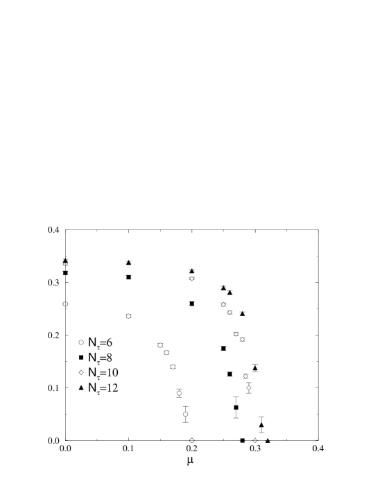
Figure 5: $\Sigma$ vs. $\mu$ on asymmetric lattices

Figure 6: Phase diagram in the $(\mu,T)$ plane

We have also studied the transition at non-zero temperature by simulations on asymmetric lattices $N_{\tau}\times 36^{2}$ with $1/g^{2}=0.75$. The results are shown in Fig. 5. The data show that the transition is softened, with $\mu_{c}$ a decreasing function of temperature, in qualitative agreement with the mean field prediction. Estimates of the location of the phase transition are plotted in Fig 6 together with the mean field prediction (14), showing reasonable agreement; the discrepancies can probably be accounted for by $O(1/N_{f})$ corrections.

There are two issues raised by the lattice simulations that are worth discussing. First, what is the order of the transition for $T>0$? The isolated nature of the first order point predicted by mean field theory seems unlikely to persist once quantum effects are included in the calculation. Indeed, the simulations showing a two-state signal characteristic of the first order transition were performed on lattices of finite extent, and by implication at a small but non-zero temperature. The most likely scenario is for the line of first order transitions to extend into the $(\mu,T)$ plane, to end at a tricritical point separating it from a line of second order transitions continuing to the point $(0,T_{c})$. This behaviour has been verified by calculation of $O(1/N_{f})$ corrections in the two dimensional model [14], although ironically, the thermodynamics in this case are not described by the $1/N_{f}$ expansion due to condensation of topological defects in the resulting one dimensional system [15][8]. Numerical studies with higher precision, or explicit calculations of $O(1/N_{f})$ corrections in three dimensions would be useful to clarify the situation further.

Secondly, what is the nature of the pure thermal phase transition, ie. along the $\mu=0$ axis? The mean field solution (13) predicts a transition with Gaussian exponents $\beta=\nu={1\over 2}$, $\delta=3$, $\gamma=1$, $\eta=0$, and indeed, early simulations [4] on a $12\times 36^{2}$ system with $N_{f}=12$ and with $m\not=0$, estimated $\delta=3.0(1)$ in apparent confirmation. This led to speculation [16] that models in which a composite field (in this case a bound fermion – anti-fermion pair) condenses violate the conventional wisdom [17], which predicts that the thermal transition has the exponents of the dimensionally reduced ferromagnetic model with the same global symmetry, in this case the two dimensional Ising model. More recently there has been an analytic study [18] using both dimensional reduction and subsequent linked cluster expansion techniques, and a more accurate numerical study [19]: both favour the $2d$ Ising model exponents for $N_{f}<\infty$.

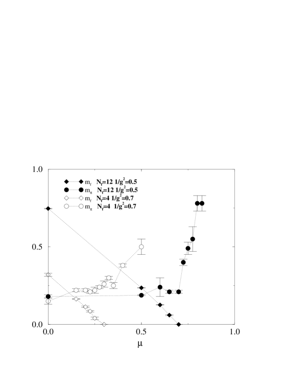
Figure 7: Spectrum results for the U(1) model

Next I turn to numerical studies of Model $B$ [10], which has a continuous U(1) chiral symmetry and hence a Goldstone pion in the broken phase. Here all simulations were performed on a $16^{3}$ system with bare mass $m=0.01$, but this time with differing numbers of flavors, ie. $N_{f}=4$ and 12 in continuum normalisation. Just as for the $\mbox{Z}_{2}$ model, it was found that a sharp chiral symmetry restoring transition occurs at a critical $\mu_{c}\sim O(\Sigma_{0})$, and that bulk expectation values of number density $\rho$ and energy density were in good qualitative agreement with mean field theory, the greater discrepancy occuring as expected for $N_{f}=4$. More interesting results come from studies of the spectrum; the fermion mass $m_{f}$ is measured by studying decay of the timeslice propagtor $G_{+}(t)$ in the timelike direction (a $\pm$ sign denotes that $G$ is calculated with a factor $\mbox{e}^{\pm\mu}$ on forward-pointing links), while the decay of the auxiliary field correlator yields the pion mass $m_{\pi}$. Results are shown in Fig. 7 for $N_{f}=12$, $1/g^{2}=0.5$ (ie. small quantum corrections, large lattice spacing), and $N_{f}=4$, $1/g^{2}=0.7$ (larger quantum effects, closer to the continuum limit).

What is observed is a clear separation between the scale defined by the critical chemical potential $\mu_{c}\sim m_{f}(\mu=0)$, and the scale $m_{\pi}/2$. This is significant, since it implies that the Gross-Neveu model does not suffer from the early onset of symmetry restoration observed in simulations of both quenched [20] and full [21] QCD. Instead we find $m_{f}(\mu)\simeq m_{f}(0)-\mu$, and $m_{\pi}$ roughly constant for $\mu<\mu_{c}$, and rising sharply for $\mu>\mu_{c}$, in accordance with naive expectation. Why should this be? The answer seems to be that the Goldstone mechanism in these models is realised through a pole in the pseudoscalar channel formed from disconnected diagrams (ie. sum of bubbles), in accord with the $1/N_{f}$ expansion. Indeed, the connected (ie. flavor non-singlet) diagram, formed from the expectation $\langle G_{+}(t)G_{-}^{\dagger}(t)\rangle$, appears numerically much less important, yielding a bound state mass of roughly $2m_{f}(0)$ [22]. If the connected diagram had been numerically dominant, as is the case in gauge theories, then the same diagram would have predicted a light state formed between two fermions of opposite axial charge (recall the discussion below eqn. (21)); since this state carries net fermion number, it would be equivalent to a baryonic pion, and hence promote a premature restoration of the symmetry as $\mu$ increases [23].

4 SUMMARY AND OUTLOOK

The Gross-Neveu model presents an “easy” problem, in the sense that it has a well-defined continuum limit, and can be explored in a controlled fashion without introducing ad hoc interactions or form factors. Nonetheless, the physics it contains for $\mu\not=0$ is rich, and is possibly not too dissimilar, at least qualitatively, from that of QCD. Issues such as the nature of the thermal transition, the existence of a tricritical point, and also a possible nucleon liquid-vapour phase transition (expected for $\mu<\mu_{c}$ for sufficiently low temperatures) can all be addressed by more thorough simulations than those reviewed here. Moreover, quantitative information is also available in principle from the $1/N_{f}$ expansion, known to be accurate for $N_{f}$ as small as 2 [6]. In addition, the model might also serve as a useful warm-up exercise for other analytic methods such as the Schwinger-Dyson or exact renormalisation group approaches. Despite its apparent easiness, however, the model also presents a non-trivial test for numerical algorithms, such as the Glasgow reweighting method [21], designed to treat systems with complex integration measures. One insight to come out of the study [22] is that the Gross-Neveu model appears to be simulable by conventional means because the Goldstone mechanism is realised in a fundamentally different way to the case in gauge theories, reflecting in turn the fact that the global symmetries of the two problems are different for general $N_{f}$.

Let me finish by advertising the fact that there is also a “difficult” problem in three dimensional fermion physics, namely the Thirring model, with the following Lagrangian density:

$${\cal L}_{Thirring}=\bar{\psi}_{i}({\partial\!\!\!/}\,+m)\psi_{i}+{g^{2}\over{2N_{f}}}(\bar{\psi}_{i}\gamma_{\mu}\psi_{i})^{2}.$$ (24)

This model has been studied by $1/N_{f}$ expansion [24], Schwinger-Dyson equations [25], and numerical simulation [26]. I believe it to be the simplest fermionic system for which a numerical solution is necessary. Its essential features are:

1. It is non-perturbative in $1/N_{f}$.

2. It exhibits dynamical chiral symmetry breaking and a UV fixed point of the renormalisation group for $N_{f}\leq 4$.

3. The chiral symmetry group is $\mbox{U}(N_{f})$, similar to QCD.

4. For $\mu\not=0$ the action is complex.

In other words, the model exhibits all the essential physics except confinement. Perhaps it would provide a suitable intermediate challenge while we wait for the means to solve the real problem.

References

- [1] D.J. Gross and A. Neveu, Phys. Rev. D10 (1974) 3235.
- [2] K.G. Wilson, Phys. Rev. D7 (1974) 2911; D.J. Gross in Methods in Field Theory, Les Houches XXVIII, eds. R. Balian and J. Zinn-Justin, (North Holland 1976); B. Rosenstein, B.J. Warr and S.H. Park, Phys. Rev. Lett. 62 (1989) 1433; Phys. Rep. 205 (1991) 59.
- [3] S.J. Hands, A. Kocić and J.B. Kogut, Phys. Lett. B273 (1991) 111.
- [4] S.J. Hands, A. Kocić and J.B. Kogut, Ann. Phys. 224 (1993) 29.
- [5] J.A. Gracey, Int. J. Mod. Phys. A6 (1991) 395; ibid. A9 (1994) 567; Phys. Lett. B308 (1993) 65; Phys. Rev. D50 (1994) 2840.
- [6] L. Kärkkäinen, R. Lacaze, P. Lacock and B. Petersson, Nucl. Phys. B415 (1994) 781, erratum B438 (1995) 650; E. Focht, J. Jersák and J. Paul, Phys. Rev. D53 (1996) 4616.
- [7] B. Rosenstein, B.J. Warr and S.H. Park, Phys. Rev. D39 (1989) 3088.
- [8] F. Karsch, J.B. Kogut and H.W. Wyld, Nucl. Phys. B280 [FS18] (1987) 289.
- [9] S.J. Hands, A. Kocić and J.B. Kogut, Nucl. Phys. B390 (1993) 355.
- [10] S.J. Hands, S. Kim and J.B. Kogut, Nucl. Phys. B442 (1995) 364.
- [11] C.J. Burden and A.N. Burkitt, Europhys. Lett. 3 (1987) 545.
- [12] Y. Cohen, S. Elitzur and E. Rabinovici, Nucl. Phys. B220 (1983) 102.
- [13] S. Duane, A.D. Kennedy, B.J. Pendleton and D. Roweth, Phys. Lett. B195 (1987) 216.
- [14] U. Wolff, Phys. Lett. B157 (1985) 303.
- [15] R.F. Dashen, S.-K. Ma and R. Rajamaran, Phys. Rev. D11 (1975) 1499.
- [16] A. Kocić and J.B. Kogut, Phys. Rev. Lett. 74 (1995) 3110.
- [17] R. Pisarski and F. Wilczek, Phys. Rev. D29 (1984) 338.
- [18] T. Reisz, in Field Theoretical Tools in Polymer and Particle Physics, Wuppertal 1997, hep-lat/9712017.
- [19] J.B. Kogut, M.A. Stephanov and C.G. Strouthos, hep-lat/9805023.
- [20] I.M. Barbour, N.-E. Behilil, E. Dagotto, F. Karsch, A. Moreo, M. Stone and H.W. Wyld, Nucl. Phys. B275 [FS17] (1986) 296; C.T.H. Davies and E.G. Klepfish, Phys. Lett. B256 (1991) 68.
- [21] I.M. Barbour, S.E. Morrison, E.G. Klepfish, J.B. Kogut and M.-P. Lombardo, Phys. Rev. D56 (1997) 7063; I.M. Barbour, these proceedings.
- [22] M.-P. Lombardo, S.E. Morrison, S.J. Hands, I.M. Barbour and J.B. Kogut, in preparation; S.E. Morrison, these proceedings.
- [23] M.-P. Lombardo, J.B. Kogut and D.K. Sinclair, Phys. Rev. D54 (1996) 2303.
- [24] M. Gomes, R.S. Mendes, R.F. Ribeiro and A.J. da Silva, Phys. Rev. D43 (1991) 3516; S.J. Hands, Phys. Rev. D51 (1995) 5816.
- [25] T. Itoh, Y. Kim, M. Sugiura and K. Yamawaki, Prog. Theor. Phys. 93 (1995) 417; M. Sugiura, Prog. Theor. Phys. 97 (1997) 311.
- [26] L. Del Debbio, S.J. Hands and J.C. Mehegan, Nucl. Phys. B502 (1997) 269.