Abstract

A new approach to the inclusion of virtual quark effects in lattice QCD simulations is presented. Infrared modes which build in the chiral physics in the light quark mass limit are included exactly and in a gauge invariant way. At fixed physical volume the number of relevant infrared modes does not increase as the continuum limit is approached. The acceptance of our procedure does not decrease substantially in the limit of small quark masses. Two alternative approaches are discussed for including systematically the remaining ultraviolet modes. In particular, we present evidence that these modes are accurately described by an effective action involving only small Wilson loops.

1 Introduction

Recent studies of the origin and role of exceptional configurations [1, 2, 3] leading to extremely noisy hadron correlators in quenched lattice QCD for light quark masses have underlined the importance of nonlocal topological fluctuations in determining the chiral physics of the quenched theory. It has been known for a long time [4] that such fluctuations completely alter the behavior of the theory in the light quark mass limit once the quark determinant is included in a full dynamical calculation. Moreover, the appearance of spurious real modes [1] of the Wilson-Dirac operator on finite lattices in association with such fluctuations accounts for the increasing frequency of exceptional configurations at stronger coupling and low quark mass. These connections all suggest that reliable calculations in the chiral limit of lattice QCD require an accurate treatment of the low eigenmodes of the quark Dirac operator.

Singularities of quark propagators in the quenched theory are automatically regulated by corresponding zeroes of the quark determinant. However, this regularization is only effective if the low eigenmodes of the quark Dirac operator are treated precisely: in particular, valence and sea quark masses must be identical. On the other hand, the high eigenmodes (corresponding to imaginary masses for scales well above the QCD scale up to the lattice cutoff) when integrated out contribute to an effective gauge-invariant gluonic action which, for physics on small momentum scales, simply amounts to a redefinition of the scale of the theory. To the extent that the ground state hadron spectrum involves hadronic bound states with constituent quarks all off-shell on the order of $\Lambda_{\rm QCD}$, it therefore seems likely that high eigenmodes are simply irrelevant for spectrum calculations, even in full QCD. By writing the fermion determinant in terms of the hermitian operator $H\equiv\gamma_{5}(D\!\!\!/(A)-m)$ [5] we are able to deal with a completely real spectrum. Moreover, the individual eigenvalues have a direct physical interpretation as a gauge-invariant measure of off-shellness of the quark fields (to see this, we recall that for the free continuum theory, the eigenvalues of $H$ are simply $\pm\sqrt{p^{2}+m^{2}}$ for a quark mode of Euclidean momentum $p$).

We shall argue in this paper that a separation of low and high eigenmodes can in fact be carried out in a practical way in unquenched lattice QCD calculations, leading to an efficient way of building in the important physics of the quark determinant in the chiral limit. Such a separation also corresponds to a completely gauge-invariant and smooth interpolation between the quenched and full dynamics of the theory. The procedure we propose also yields as a byproduct very detailed and useful information about the infrared spectrum of the Dirac operator which is known to be intimately related to the chiral physics of the theory [6], and central to the overlap formulation [7] of lattice QCD.

In Section 2 we describe a regularized version of the fermionic determinant which interpolates smoothly between the quenched and full theory, in a way which allows for the selective inclusion of fermionic modes in a predetermined momentum range (typically from zero up to a given cutoff $\mu$). This regularization is amenable to an analytic perturbative calculation in which the role of the high eigenmodes contributing to the full fermionic determinant can be clearly isolated. Such a regularization can be studied analytically in abelian 4D gauge theory, where the $\mu$-dependence of the determinant for large $\mu$ and low momentum is seen to reduce to a shift of bare coupling (or in the lattice context, of scale).

In Section 3 we describe the results of some simulations in 2 dimensional lattice QED (QED2), which has proven to be an extremely useful testbed for exploring features of the Dirac-Wilson spectrum in lattice gauge theory. Here, and henceforth in all the numerical simulations, we employ a regularization of the fermionic determinant in terms of a sharp mode cutoff which is physically equivalent to the smooth regularization of Section 2 but suitable for numerical implementation in large systems. It is shown that the fluctuations of the full fermionic determinant in an exact dynamical simulation of QED2 are essentially restricted to a small fraction (for the lattices studied here, essentially the lowest few percent) of the spectrum. Comparisons of pseudoscalar correlators computed in the quenched and full dynamical theory are made with an approximate simulation where only the lowest ten percent of the eigenvalues of the hermitian operator $\gamma_{5}(D\!\!\!\!/-m)$ are included in the fermionic determinant. The truncated determinant simulations essentially reproduce the full dynamical results. Two characteristic features of unquenched gauge theory, the suppression of topologically nontrivial sectors and the breaking of the string due to shielding, are also illustrated using the truncated determinant approach in QED2. Of course, in the case of QED2, the superrenormalizability of the theory implies that the high eigenmodes are basically inert, in distinction to the case in 4D gauge theory where these modes will necessarily introduce a further logarithmic rescaling due to the variable screening effect of virtual quark/antiquark pairs at different length scales.

In Section 4 we describe in detail the algorithm we have employed for the simulations of full QCD (on a 12³x24 lattice at $\beta$=5.9 and inverse lattice spacing $a^{-1}=$1.78 Gev for the quenched theory) with a truncated determinant. The Lanczos procedure allows reliable extraction of Dirac eigenmodes up to energies $\sim$370 MeV, certainly enough to include the essential low energy chiral physics of QCD. Moreover, the Lanczos procedure extracts the needed small eigenvalues rapidly as the spectrum is relatively sparse there. Unlike the case of propagator inversion, the Lanczos method is stable even in the presence of very small eigenvalues provided these are not too dense. We also discuss some aspects of the Monte Carlo dynamics (acceptance rate and equilibration time) for our update procedure, in which pure gauge heat bath sweeps alternate with Metropolis accept/reject steps for the truncated determinant. A crucial point is that we do not see a dramatic fall in the acceptance rate of our procedure as we go to lighter quark masses.

In Section 5 we present the results of our truncated determinant simulations of QCD4. The initial study involves runs on a 12³x24 lattice at $\beta$=5.9 and at three kappa values (0.1570, 0.1587 and 0.1597), reaching in the lightest case a pion mass on the order of 280 MeV. Pseudoscalar meson masses are measured and a value for the critical hopping parameter extracted. The inclusion of 100 quark eigenmodes (all modes up to $\sim$370 MeV) eliminates the necessity for considering quenched chiral logs [8] in the chiral extrapolations. The topological charge distribution is measured for different quark masses and compared with the quenched result. As expected, nonzero topological charge is strongly suppressed in the light quark limit. Measurements of the string tension reveal clearly a screening of the quark-antiquark potential from the virtual sea quarks, although the lattice used is still too small to allow us to see the asymptotic flattening expected at large distances.

In Section 6 we show that the high momentum modes can be included in a precise way by a combination of the truncated determinant and multiboson methods [9]. The procedure suggested in this paper is in a sense exactly complementary to the multiboson approach of Lüscher. The latter approach treats the high eigenmodes of the Dirac operator very well, but necessarily introduces errors whenever small eigenvalues are present. In the chiral limit such modes become frequent and in fact dominate the chiral physics. Here we propose treating these modes as precisely as possible. Another approach to the inclusion of the high modes, a loop Ansatz for the short distance piece of the quark determinant, is also discussed in this final section. Such an Ansatz, involving relatively short Wilson loops (up to length 6), is shown to give a very accurate description of the high end of the quark determinant. Finally, in Section 7 we summarize our conclusions.

2 Truncated determinants in gauge theory

The separation of low and high eigenmodes in the fermionic determinant can be accomplished in an analytically convenient way by smoothly switching off the higher eigenvalues above a sliding momentum scale $\mu$. Given a matrix ${\cal M}$ then ${\rm det}(\tanh({\cal M/\mu}))$ reduces to unity for $\mu$ much below the smallest eigenvalue of ${\cal M}$ while reproducing the full determinant (up to an irrelevant multiplicative factor) for $\mu$ much above the highest eigenvalue. For a gauge theory, defining the hermitian operator $H\equiv\gamma_{5}(D\!\!\!/(A)-m)$, then the effective action obtained from integrating out each flavor of fermion of mass $m$ can be regularized as the logarithm of the smoothly truncated determinant

$${\cal D}(\mu) \equiv \frac{1}{2}{\rm tr}\ln(\tanh(\frac{H^{2}}{\mu^{2}}))$$ (1)

$$= {\rm tr}\{\ln(1-e^{-2H^{2}/\mu^{2}})-\ln(1+e^{-2H^{2}/\mu^{2}})\}$$ (2)

This definition allows an analytic calculation of the regularized determinant in weak coupling perturbation theory, which describes the $\mu$-dependence of ${\cal D}(\mu)$ for $\mu$ well above the QCD scale. The calculation can be carried out for a nonabelian lattice regularized theory, but we shall illustrate the procedure here for the case of a continuum 4-dimensional abelian gauge theory. Note that

$$H^{2} = K_{0}+K_{1}+K_{2}$$ (3)

$$K_{0} \equiv \Box+m^{2}$$ (4)

$$K_{1} \equiv \{-i\partial\!\!\!/,A\!\!/\}$$ (5)

$$K_{2} \equiv A_{\mu}A_{\mu}$$ (6)

To second order in weak coupling perturbation theory, we may compute ${\cal D}(\mu)$ by expanding to first order in $K_{2}$ and to second order in $K_{1}$. The calculation is lengthy but straightforward (details will be given elsewhere)- here we quote the result only. Expressed in terms of momentum space fields, one finds

$${\cal D}=\int\frac{d^{4}k}{(2\pi)^{4}}\beta(k^{2},m,\mu)A_{\mu}(k)(k^{2}\delta_{\mu\nu}-k_{\mu}k_{\nu})A_{\nu}(-k)$$ (7)

The contribution of the high modes can be studied by taking $\mu$ large compared with the quark mass $m$ and, in the nonabelian case, with the QCD scale. Then these modes affect the low energy physics (i.e for $k<<\mu$) through the low momentum limit of $\beta(k^{2})$. Explicit calculation gives

$$\beta(k^{2},m,\mu)\simeq-\frac{1}{24}\ln(\frac{\mu^{2}}{m^{2}})+O(k^{2})$$ (8)

which exactly corresponds to the expected $\mu$-dependence of the screening shift in the running coupling induced by virtual fermionic modes in the momentum range up to $\mu$.

The decoupling of the high fermionic modes suggests that lattice QCD calculations performed at weak enough coupling should be insensitive to the fluctuations induced by eigenvalues of the Dirac operator much above the QCD scale, except for an overall shift in the scale of the theory induced by renormalizations of the coefficients of the low dimension operators making up the effective pure gauge action. In particular, dimensionless ratios of physical quantities should fairly soon become insensitive to inclusion of higher modes in the fermionic determinant. In a superrenormalizable theory like QED2, this insensitivity should even be apparent in dimensionful quantities, as we do not have a logarithmic running of scale in this case.

3 Truncated Determinant Algorithm in QED2

Abelian gauge theory in 2 space-time dimensions (the massive Schwinger model) has proven to be a marvellously manageable testbed for exploring in detail [10, 2] the spectral properties of the Dirac-Wilson operator. The computational expense of performing even exact update full dynamical simulations is relatively slight, essentially full information on the spectrum can be obtained configuration by configuration, and the system mimics, at least qualitatively, many of the topological and chiral properties of 4 dimensional QCD. This model also turns out to be a very useful starting point for investigating the relative importance of the infrared and ultraviolet ends of the Dirac spectrum in a full dynamical lattice simulation.

Although the calculation of all the eigenvalues of $H$, and hence of ${\cal D}(\mu)$ as defined in the previous section, is perfectly feasible for 2D QED, the restriction of practical numerical techniques for the much larger matrices of 4D QCD to the low-lying eigenvalues suggest the use of a simpler truncation of the determinant, in which the lowest (in absolute magnitude) $N_{\lambda}$ positive and negative eigenvalues of $H$ are included and all higher modes dropped. As we shall see in Section 5, precisely such a truncation scheme matches on exactly to a very accurate representation of the high end of the determinant in terms of an effective loop action. Labelling positive eigenvalues of $H$ as $\eta_{n}$ and negative eigenvalues as $\zeta_{n}$ (where the index runs in the direction of increasing absolute magnitude) we define

$${\cal D}(N_{\lambda}) \equiv \frac{1}{2}\sum_{n=1}^{N_{\lambda}}\ln(\eta_{n}^{2}\zeta_{n}^{2})$$ (9)

$$\hat{\cal D}(N_{\lambda}) \equiv \frac{1}{2}\sum_{n=N_{\lambda}+1}^{D}\ln(\eta_{n}^{2}\zeta_{n}^{2})$$ (10)

where 2$D$ is the dimensionality of the discrete Wilson-Dirac matrix for the lattice theory. An exact full dynamical simulation would include the full (log) determinant ${\cal D}(N_{\lambda})+\hat{\cal D}(N_{\lambda})$ in the effective gauge action. The extent to which the low eigenvalues determine the physics of the unquenched theory can be examined by comparing the fluctuations- in a dynamical simulation- of ${\cal D}(N_{\lambda})$ with those of $\hat{\cal D}(N_{\lambda})$ for various choices of $N_{\lambda}<<D$. These fluctuations are shown graphically in Fig.1, for 40 configurations generated in a full dynamical simulation using an exact update algorithm. In Fig.2 the fluctuations are shown for 40 configurations in a quenched simulation. The lattice used was 10x10 at $\beta$=4.5 with a bare quark mass of 0.095. Evidently the fluctuations are essentially all confined to the low end of the spectrum. In the quenched case the size of the fluctuations at the infrared end is considerably larger than for the dynamical configurations, as configurations with small eigenvalues are suppressed once the determinant factor is included in the update procedure. The appearance of such configurations is intimately related to the exceptional configurations encountered in quenched calculations at strong coupling and/or small quark mass.

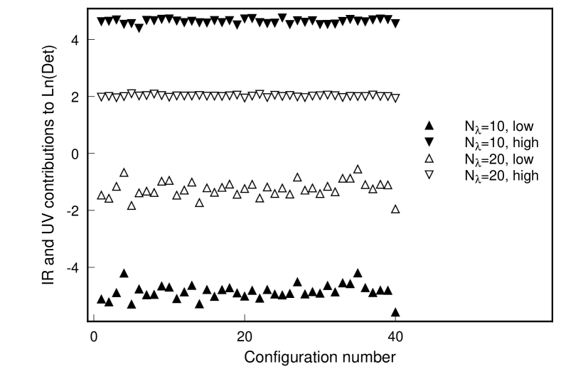
Figure 1: Fluctuations in ${\cal D}(N_{\lambda}),\hat{\cal D}(N_{\lambda})$, dynamical configurations. For ease of visibility, the curves have been shifted vertically.

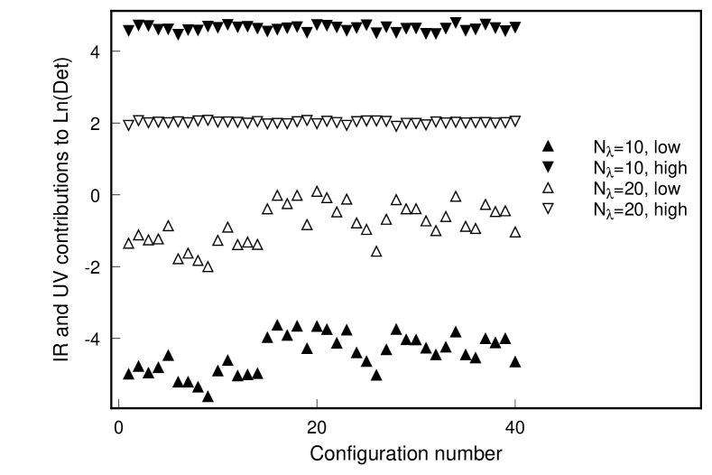
Figure 2: Fluctuations in ${\cal D}(N_{\lambda}),\hat{\cal D}(N_{\lambda})$, quenched configurations

This behavior suggests an approximate unquenched algorithm in which only ${\cal D}(N_{\lambda})$ is used in the determinant part of the effective lattice action. If $N_{\lambda}$ is chosen large enough, all the nonperturbative infrared physics will be properly included. Exceptional configurations, in which there is an anomalously low eigenmode of the Dirac-Wilson operator, are tamed in the expected way [11], and the convergence of the procedure can be examined simply by repeating the run for increasingly large $N_{\lambda}$. The update algorithm we have chosen is very simple: a number (typically 5) of conventional Monte Carlo (Metropolis) sweeps are performed to obtain a new gauge configuration, a new value for ${\cal D}(N_{\lambda})$ is calculated (for QED2 on a 10x10 lattice, we can easily obtain all the eigenvalues by direct diagonalization) and compared with that for the preceding configuration. Then the truncated determinant factor is used to provide a Metropolis accept/reject criterion for the gauge configuration update. With $N_{\lambda}$=10, the acceptance ratio was typically in the range of 50-75%. Measured quantities such as the pseudoscalar correlator decorrelated after a few configuration updates (the statistical errors shown include autocorrelation times computed from the data). The results of such a procedure for the pseudoscalar correlator are shown in Fig 3 for a quark mass (lattice units) of 0.05. For such a small mass, using Wilson fermions, the quenched functional integral is dominated by real pole contributions which appear in the simulation as wildly noisy values for the correlators (one finds in a typical run of 800 sweeps values for the pion propagator at zero time separation ranging from several thousand to zero, for a quantity averaging to order unity in the dynamical theory). Instead we have plotted the quenched results regularized by the pole shifting (or “modified quenched approximation”) procedure of [1]. Evidently the full dynamical result for the pseudoscalar correlator is reached with only a small fraction (in this case, about 10%) of the eigenmodes included in the fermionic determinant. When only 5% of the eigenvalues are included, the result is intermediate between the quenched and full dynamical values.

Figure 3: Comparison of quenched, full dynamical and truncated determinant simulations: 10x10 lattice, $\beta$=4.5, m=0.05

As we are working at a very small value of quark mass, it is also of interest to study the effect of the truncated determinant factor on the topological charge distribution and the string tension of the theory. For the quenched simulations on a 10x10 lattice at $\beta=$4.5, the topological charge, defined as

$$Q_{\rm top}\equiv\frac{1}{2\pi}\sum_{P}\sin{(\theta_{P})}$$ (11)

(where $\theta_{P}$ is the plaquette angle for plaquette $P$), is found to be concentrated at roughly integer values, with charges 0 and 1 dominating. The histogram of topological charge values obtained from 800 quenched configurations is shown in Fig. 4. As low eigenvalues are introduced via the truncated determinant, the nonzero topological charge configurations are suppressed. Again, with $N_{\lambda}$=5, the resulting distribution is hardly distinguishable from the full dynamical result.

Figure 4: Topological charge distribution for quenched, full dynamical and truncated determinant simulations: 10x10 lattice, $\beta$=4.5, m=0.05

The quark-antiquark potential determined for two different sea quark masses (bare mass 0.06 and 0.10) is shown in Fig 5. The calculation was done in the truncated theory on a 16x16 lattice at $\beta$=4.5 using $N_{\lambda}$=10 eigenvalues. Also shown is the exact result for the quenched theory and exact update full dynamical theory (at sea quark mass 0.06). The small eigenvalues properly represent the large loops induced by the determinant, leading to a breaking of the string at longer distances for light quarks.

Figure 5: Quark-antiquark potential in QED2.

4 Calculating Truncated Determinants in Large Sparse Systems

There are a number of techniques available for the extraction of a limited number of low eigenvalues of a large sparse linear system: most popular are conjugate gradient approaches [12], or the Lanczos technique [13], suitably modified to guard for the appearance of spurious eigenvalues [14]. The latter approach has been studied extensively by Kalkreuter [15], and has proven to be most well suited for the task at hand, namely, the accurate extraction of a complete set of low-lying eigenvalues of $\gamma_{5}(D\!\!\!/-m)$ up to an energy scale which ensures that all the important soft chiral dynamics of full QCD is included in the Monte Carlo simulation. Typically, on lattices of physically interesting volume in 4D QCD, this requires the determination of something on the order of 100 eigenvalues. One advantage of the Lanczos approach is that it can be pushed through to the determination of as many eigenvalues as desired, with a numerical effort which grows empirically as roughly the square of the desired energy cutoff (in the portion of the spectrum corresponding to the physical branch). In particular, on small lattices, it is relatively straightforward to determine the entire spectrum, which is useful both for diagnostic purposes and in studying the systematic effects of an algorithm based on a truncated determinant.

The Lanczos technique is a standard part of the literature in Numerical Analysis (see, for example, [13]) so we shall give only a very brief review of the procedure here. Given a hermitian matrix $H$ (in our case, this is just the matrix $\gamma_{5}(D\!\!\!/-m)$ discussed previously), a series of orthonormal vectors $v_{1},v_{2},v_{3}...$ are generated from a starting vector $w_{0}\equiv v_{1}$ by the following recursion:

$$v_{n+1} = w_{n}/\beta_{n}$$ (12)

$$n \rightarrow n+1$$ (13)

$$\alpha_{n} = (v_{n},Hv_{n})$$ (14)

$$w_{n} = (H-\alpha_{n}I)v_{n}-\beta_{n-1}v_{n-1}$$ (15)

$$\beta_{n} = \sqrt{(w_{n},w_{n})}$$ (16)

where $\alpha_{n},\beta_{n}$ are real numbers (by virtue of the hermiticity of $H$), and the initial conditions are $\beta_{0}=1,v_{0}=0$. It is straightforward to verify that the matrix of $H$, in the basis spanned by the Lanczos vectors $v_{n}$ is tridiagonal, with the numbers $\alpha_{1},\alpha_{2},..$ down the main diagonal, and the numbers $\beta_{1},\beta_{2},..$ on the first super- (and sub-)diagonals. If the Lanczos recursion is carried to order $N$, one is thus led to a $N$x$N$ truncation of the original linear system, and the eigenvalues of the resulting tridiagonal matrix $T^{(N)}$ represent increasingly accurate approximants to the eigenvalues of the full system, provided only that the starting vector $w_{0}$ is not entirely contained in an invariant subspace of $H$. Typically, $w_{0}$ is chosen randomly and one expects that such a random vector will overlap nontrivially with all the eigenvectors of $H$.

There are several features of the Lanczos procedure which appear at first sight problematic but which nevertheless turn out not to compromise its efficacy in the present application. First, degenerate eigenvalues of the original matrix $H$ are not properly handled (although methods have been devised for circumventing this drawback [13]). This turns out to be irrelevant in our QCD application as the generic spectrum of $H\equiv\gamma_{5}(D\!\!\!\!/-m)$ for a typical gauge configuration encountered in the course of a Monte Carlo simulation is entirely nondegenerate. Secondly, the effects of roundoff error in the algorithm can be quite severe, and lead to the appearance of spurious eigenvalues and to the false duplication of real eigenvalues. Fortunately a simple and effective cure for this problem, first suggested by Cullum and Willoughby [14], proves to be practical in the gauge theory case [15]. However, it remains an unfortunate feature of the algorithm that the number of accurate eigenvalues extracted at level $N$ of the recursion is typically considerably smaller than $N$. For example, on a 12³x24 lattice at $\beta$=5.9, the extraction of the lowest 100 eigenvalues of the Dirac operator typically requires on the order of 10,000 Lanczos sweeps. (The computational cost of a single Lanczos sweep is essentially that of the single $D\!\!\!/$ multiplication incurred in producing the next Lanczos vector $w_{n}=Hv_{n}+..$.) Finally, although the diagonalization of a tridiagonal matrix is conceptually trivial and efficiently implementable by scalar algorithms (e.g. by a QL implicit shift algorithm [18]), the parallel implementation of this procedure is not entirely trivial. In our simulations, this is essential to avoid a serious bottleneck in the simulation when tridiagonal matrices of order up to several tens of thousands must be efficiently processed. We describe below an elegant parallel approach to the extraction of the spectrum of $T^{(N)}$.

In the case of the Dirac operator in QCD, the choice of the random vector $w_{0}$ used to start the recursion appears to be fairly innocuous (a local source seems perfectly adequate, for example) . An important check that the spurious eigenvalues are correctly identified and that the remaining “good” eigenvalues are sufficiently converged relies on the gauge-invariance of the individual eigenvalues of $H$ which can be verified explicitly by recomputing the eigenvalues with varying degrees of gauge-fixing. We have performed extensive checks to ensure that the eigenvalue spectrum, and a-fortiori the truncated determinant ${\cal D}(N_{\lambda})$, is invariant (typically to at least 8 significant figures) under gauge transformations of the input configuration.

The procedure we use to isolate converged eigenvalues of $H$ involves two stages. First, spurious eigenvalues are identified by the procedure of Cullum and Willoughby- namely, eigenvalues of the tridiagonal matrix $T^{(N)}$ are compared with those of the matrix $\hat{T^{(N)}}$ obtained by deleting the first row and column of $T^{(N)}$ and removing all common eigenvalues of the two systems. Secondly, converged eigenvalues are identified by requiring either duplication of the remaining good eigenvalues or stability within a preassigned precision level when eigenvalues are compared at recursion level $N-N_{\rm gap}$ and $N$. Typically we insist on a precision level of at least 10^-5 and choose $N_{\rm gap}$=100. The above procedure requires the resolution of the central part of the eigenvalue spectrum for four large tridiagonal matrices (of dimension $N$,$N$-1,$N-N_{\rm gap}$, and $N-N_{\rm gap}$-1, respectively). It is therefore highly desirable to perform these diagonalizations in a way that allows parallelization.

The key to extracting the central part of the spectrum of a tridiagonal matrix in a parallel machine lies in the Sturm Sequence property of such matrices [13], valid provided none of the subdiagonal entries $\beta_{n}$ vanish, as is certainly the case for generic gauge configurations. Let $p_{n}(\lambda)$ be the secular determinant ${\rm det}(T^{(N)}_{n}-\lambda I)$ of the $n$x$n$ principal submatrix $T^{(N)}_{n}$ of $T^{(N)}$. Then the number of eigenvalues of $T^{(N)}$ less than any preassigned $\lambda$ equals the number of sign changes in the sequence $p_{0}(\lambda),p_{1}(\lambda),...p_{N}(\lambda)$. As the $p_{n}(\lambda)$ can readily be calculated by a simple two term recursion relation, an obvious bisection procedure can be used to determine the $n$’th eigenvalue of $T^{(N)}$ at any desired level of precision. Moreover, the task of extracting different eigenvalues can be assigned completely independently to separate processors, provided global access to the elements $(\alpha_{i},\beta_{i})$ of $T^{(N)}$ is arranged.

Figure 6: Spectral density,$\beta$=5.9,$\kappa$=0.1587

In Fig 6 we show the spectrum of $H$ for a typical configuration on a 12³x24 lattice at $\beta$=5.9, $\kappa$=0.1587. In this case an extended Lanczos recursion was carried out up to order $N$=78000, yielding 1478 converged eigenvalues in the central region of the spectrum. Converting the gauge-invariant eigenvalues of $H$ to a physical energy scale (using the scale $a^{-1}$=1.78 GeV from the charmonium spectrum), this corresponds to all quark eigenmodes up to 970 MeV. The energy reach as a function of number of Lanczos sweeps for this lattice is shown in Fig 7. In the simulations reported below, we have typically used 9500-12000 Lanczos sweeps (with slightly different tunings of the Cullum-Willoughby procedure) and included the lowest 100 (i.e. 50 positive and 50 negative) eigenvalues of $H$ in the update procedure. This cutoff corresponds to inclusion of quark eigenmodes up to an energy of approximately 370 MeV. Lanczos recursion to order $N\sim$10000 requires (for a 12³x24 lattice) about an hour on 64 nodes of the Fermilab ACPMAPS system.

Figure 7: Lanczos convergence,$\beta$=5.9,$\kappa$=0.1587

Figure 8: Determinant relaxation,$\beta$=5.7,$\kappa$=0.1685,$N_{\lambda}$=30

Figure 9: Determinant relaxation,$\beta$=5.9,$\kappa$=0.1587,$N_{\lambda}$=100

The relaxation of the determinant from its typical quenched value to the equilibrium value appropriate for the system simulated with the truncated determinant is shown in Figs. 8 and 9. On a small lattice, (6⁴ at $\beta=5.7$, $\kappa$=0.1685) a dynamical run including $N_{\lambda}=$30 eigenvalues (or up to about 500 MeV in quark mode energy) was performed, with a determinant update accept/reject every 3 heat-bath sweeps of the lattice. The resulting evolution of ${\cal D}(N_{\lambda})$ starting from a quenched configuration is shown in Fig 8. The same evolution is shown for a run on a 12³x24 lattice at $\beta$=5.9, $\kappa$=0.1587 with $N_{\lambda}=$100 in Fig 9, and with determinant accept/reject every 2 heat-bath sweeps.

The procedure we have used does not show a very strong dependence of the acceptance rate on the quark mass (fortunately!). For the heaviest quark mass studied at $\beta=$5.9, $\kappa=$0.1570 (slightly lighter than the strange quark), the acceptance rate for a run with determinant accept/reject performed every two gauge heat bath sweeps was 40%. For the lightest two quark masses ($\kappa$=0.1587 and 0.1597) two separate runs were performed with determinant accept/reject steps separated by either one or two heat-bath sweeps. For the heavier case, $\kappa$=0.1587 (corresponding to a pion mass of around 400 MeV), the acceptance was on the order of 37% for new configurations separated by 2 heat-bath sweeps, and 57% for configurations separated by a single heat-bath sweep. For the lighter mass, $\kappa$=0.1597, (corresponding to a pion mass of around 280 MeV) the acceptance was 30% for new configurations separated by 2 sweeps, and 43% for those separated by a single heat-bath sweep.

5 Simulations in QCD4

To test the efficacy of the truncated determinant approach to unquenched QCD we have performed some preliminary runs on a 12x³x24 lattice at $\beta$=5.9, for two degenerate flavors of dynamical quarks at hopping parameter values $\kappa=$ 0.1570, 0.1587 and 0.1597. For the heaviest mass, $\kappa=$0.1570, propagators were computed for every fifth configuration (60 in all), and determinant accept/reject performed after every two heat-bath gauge updates. For the lighter two masses, we also performed parallel runs with determinant accept/reject after every heat-bath sweep and with propagators measured every tenth configuration. Our results are based on 104 propagators for $\kappa=$0.1587 and 88 propagators for $\kappa=$0.1597. As fluctuations in the large distance behavior at light quark masses grow, the run at $\kappa=$0.1597 is continuing and results with much higher statistics will be presented in a later work.

Pseudoscalar meson masses were determined by measuring meson correlators with a smeared source and local sink and doing a fully correlated Euclidean time fit in the time window 8-11. At kappa values $\kappa$=0.1570, 0.1587, and 1597, the pion masses were found to be (lattice units) $M_{\pi}=$ 0.339$\pm$0.011, 0.241$\pm$0.019 and 0.198$\pm$ 0.069. The extrapolation to zero pion mass gives a critical kappa value of $\kappa_{c}\approx$0.1602, slightly higher than the pure quenched value of $\kappa_{c}$=0.15972 found in previous calculations [16]. With this critical kappa, the pion mass corresponding to our lightest case should be about 0.157 (lattice units), which converts to about 280 MeV using the scale determined for the quenched theory at this beta. We do not expect the scale in the truncated determinant simulation to be much changed from the quenched theory as the shift in beta in full dynamical simulations (see [17]) is due to a large logarithm accumulated from quark modes all the way up to the lattice cutoff, whereas the truncated determinant included here only takes into account the infrared modes up to 370 MeV. Higher statistics are presently being accumulated at the lightest quark mass, where the fluctuations in the large time meson correlators are largest.

An important aspect of the low energy chiral dynamics of QCD is the response of the topological structure of the theory to the presence of light dynamical quarks. Integrating the vacuum expectation value of the U(1) axial anomaly in QCD yields immediately, in the continuum, the anomalous chiral Ward identity

$$m_{q}\int d^{4}x<\bar{\psi}(x)\gamma_{5}\psi(x)>=\frac{1}{32\pi^{2}}\int d^{4}xF_{\mu\nu}\tilde{F}_{\mu\nu}\equiv Q_{\rm top}$$ (17)

We may therefore define a topological charge on the lattice by simply evaluating the left-hand-side of the above equation configuration by configuration. The advantage of this definition is that the required information is already immediately accessible: the Euclidean vacuum expectation value $\int d^{4}x<\bar{\psi}(x)\gamma_{5}\psi(x)>$ reduces to the trace of the inverse of $H\equiv\gamma_{5}(D\!\!\!/-m)$, the low eigenvalues of which were extracted in the course of the simulation. Namely, we have the following lattice definition of $Q_{\rm top}$

$$Q_{\rm top}\equiv\frac{1}{2\kappa}(1-\frac{\kappa}{\kappa_{c}})\sum_{i=1}^{N}\frac{1}{\lambda_{i}}$$ (18)

where the matrix dimension of $H$ is $N$ and $\lambda_{i}$ are the eigenvalues of $H$.

As the larger eigenvalues occur roughly as equal and opposite pairs, this sum actually saturates quickly at the low end, and the 100 eigenvalues computed already in the course of the simulation suffices to determine $Q_{\rm top}$ to a few percent. An example of the convergence of this spectral sum, with the mode eigenvalues converted to a physical energy scale (recall that the inclusion of 100 eigenvalues corresponds to modes up to about 370 MeV), is shown in Fig 10 for a typical configuration.

Figure 10: Convergence of the topological charge spectral sum for a typical configuration

With the definition (18), the qualitative effect of the quark determinant on the topological charge distribution can readily be studied. Two effects are clearly visible in our data:

(1) The real mode artifacts characteristic of quenched Wilson gauge theory, and which underly the increasingly frequent appearance of exceptional configurations as one goes to lighter quark masses, do not occur. Configurations with very small eigenvalues of $H$ are suppressed by the determinant factor which is driven strongly negative for any such configuration. In Fig 12 this effect is seen comparing the topological charge distribution for a dynamical run at $\kappa=0.1587$ (including the lowest 100 modes) with a completely quenched run at the same valence quark mass, Fig 11. The distributions are broadly similar (although the dynamical one is slightly narrower) but the outlying points corresponding to very large values of $Q_{\rm top}$ (i.e to the appearance of an exactly real mode of the Wilson-Dirac operator very close to the chosen kappa value) are eliminated in the dynamical run. In fact in the quenched case there are several outlying points (the furthest out at $Q_{\rm top}$ = -91.6) not shown on the figure. For the dynamical run only charges $|Q_{\rm top}|<5$ are seen.

Figure 11: The topological charge frequency distribution computed for $\kappa$ = .1587 using 100 decorrelated quenched QCD configurations on a 12³x24 lattice at $\beta$ = 5.9.

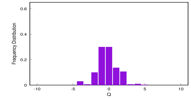
Figure 12: The same topological charge frequency distribution for 300 configurations generated by the truncated determinant algorithm with sea quark mass $\kappa=$ .1587 on a 12³x24 lattice at $\beta=$ 5.9.

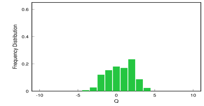
Figure 13: The topological charge frequency distribution with sea quark mass $\kappa=$ .1570. (Other parameters as in the previous figure.)

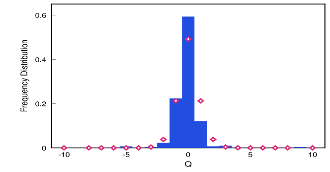
Figure 14: The same topological charge frequency distribution with sea quark mass $\kappa=$ .1597. The expected distribution from chiral perturbation theory is shown with diamonds.

(2) Nonzero topological charge must be suppressed in the chiral limit of vanishing quark mass, so we expect that the histogram of measured topological charges will narrow as one approaches $\kappa_{c}$. This effect is shown in Figs. 13 and 14 where the topological charge distribution is compared for two dynamical runs at the lowest and highest quark masses studied ($\kappa$= 0.1597 and 0.1570). The narrowing of the distribution for the lighter mass is immediately apparent. For comparison we plot the analytic result predicted by the chiral analysis of Leutwyler and Smilga [6] in the light quark limit for two degenerate flavors:

$$P(Q)=I_{Q}(x)^{2}-I_{Q+1}(x)I_{Q-1}(x)$$ (19)

with $x\equiv\frac{1}{2}VF_{\pi}^{2}M_{\pi}^{2}$. Here $V,F_{\pi},M_{\pi}$ denote the lattice space-time volume, the pseudoscalar decay constant and the pion mass respectively, all in lattice units. For $\kappa$=0.1597 we have taken $M_{\pi}$=0.15 and $F_{\pi}$=0.07 (the latter number is extrapolated from high statistics quenched runs for this lattice [16]).

The presence of low-momentum virtual sea-quark modes in the simulation should result in screening of the quark-antiquark potential extracted from Wilson loops at large distance. In Fig 15 the potential obtained in the quenched theory on a 12³x24 lattice at $\beta=$5.9 (200 configurations) is compared with that calculated from our dynamical configurations at the lightest sea quark mass ($\kappa=$0.1597). The effect of screening is clear although asymptotic flattening of the potential on this lattice occurs at distances where statistical fluctuations as well as finite volume effects dominate.

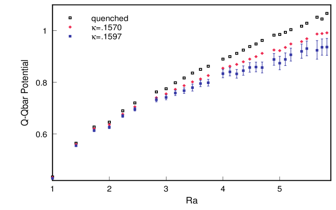
Figure 15: Quark-antiquark potential for quenched theory and dynamical theory with sea quark kappa values 0.1570, 0.1597. Error bars shown only for lightest mass (errors are largest for this case).

6 Matching the High Eigenvalues

Because QCD in four dimensions is only renormalizable, not super-renormalizable, the fluctuations of the fermion determinant are significant at all physical scales. Therefore, unlike QED in two dimensions, it can not in general be sufficient to compute accurately only the low eigenvalues of the fermionic determinant. Fortunately the short distance behaviour of QCD is very well understood. This should allow the identification of the important degrees of freedom and lead to a method for including the effects of the higher eigenvalues into the Monte Carlo process. In particular, we know that for sufficiently high momentum scales this physics should be accurately described by an improved gauge action involving Wilson loops on short distance scales only.

The fermion determinant can be separated into two pieces

$$\ln{\rm det}H=[{\rm Tr}\ln H]_{low\;\lambda}+[{\rm Tr}\ln H]_{high\;\lambda}$$ (20)

where the lowest $n_{\rm cut}$ eigenvalues are directly calculated and included in the Monte Carlo updating procedure. The contribution of the vast majority of the larger eigenvalues can be included by some approximation to the high end that (1) matches onto the low eigenvalue results without gaps or double counting, (2) is controlled and (3) becomes exact in the continuum limit. We can define the difference $\Delta$ between the approximate action, denoted $S_{a}$, and the exact contribution of the high eigenvalues, $S_{t}\equiv[{\rm Tr}\ln H]_{high\;\lambda}$ as follows:

$$\Delta=S_{t}-S_{a}$$ (21)

Any acceptable method must ensure that this difference is small ($\leq 1$) for each configuration. Therefore, we will demand that the variance of $\Delta$ for any set configurations is less than unity. Actually, we will find that a relatively simple effective loop action yields values of $\Delta$ considerably less than unity for interesting values of $n_{\rm cut}$.

Two numerical methods suggest themselves for calculating the high eigenvalues of the fermion determinant:

• The multiboson approach of Lüscher[9].

• Using a small number of gauge loops to model the determinant as proposed by Sexton and Weingarten [19], and Irving and Sexton [20].

One method to compute the high eigenvalues which is guaranteed to succeed is the multiboson approach of Lüscher[9]. Define

$$P_{eff}(U)\equiv[{\rm det(D+m)}]^{n_{f}}\exp{(-S_{g}(U))}$$ (22)

and

$$H=\gamma_{5}{\rm(D+m)}/[{\rm c_{m}(8+m)}]\;\;\;(c_{m}\geq 1)$$ (23)

where $c_{m}$ is chosen so that the eigenvalues of $H$ are in the interval $(-1,1)$. Consider two flavors of light Wilson-Dirac quarks ($n_{f}=2$). Lüscher chooses a sequence of polynomials $P_{n}(s)$ of even degree n such that

$$\lim_{n\rightarrow\infty}P_{n}(s)=1/s\;\;\;{\rm for\;\;all\;\;}0<s\leq 1$$ (24)

then

$${\rm det}H^{2}=\lim_{n\rightarrow\infty}[{\rm det}P_{n}(H^{2})]^{-1}$$ (25)

Choose polynomials such that complex roots $z_{1}\dots z_{n}$ come in complex conjugate pairs (non real) so that $\sqrt{z}=\mu+i\nu$. Then

$$P(H^{2})=const\prod_{k=1}^{n}[(H-\mu_{k})^{2}+\nu_{k}^{2}]$$ (26)

and

$${\rm det}H^{2}=\lim_{n\rightarrow\infty}\prod_{k=1}^{n}{\rm det}[(H-\mu_{k})^{2}+\nu_{k}^{2}]^{-1}$$ (27)

Hence we can finally write

$$P_{eff}(U)=\lim_{n\rightarrow\infty}\frac{1}{Z_{b}}\int D\phi D\phi^{\dagger}\exp{-S_{b}(U,\phi)}$$ (28)

where the bosonic action is given by

$$S_{b}=S_{g}(U)+\sum_{k=1}^{n}\sum_{x}|(H-\mu_{k})\phi_{k}(x)|^{2}+\nu^{2}|\phi_{k}(x)|^{2}.$$ (29)

To estimate how many boson fields are required to represent the original action to a fixed accuracy in the range ($\epsilon<s\leq 1$) Lüscher considered polynomials of the Chebyshev type (denoted T). Defining $u=(s-\epsilon)/(1-\epsilon)$ and $\cos\theta=2u-1$, $T^{\star}_{r}(u)=\cos(ru)$ and we can write

$$P(s) = [1+\rho T^{\star}_{n=1}(u)]/s$$ (30)

$$R(s) = [P(s)-(1/s)]s(\epsilon<s\leq 1)$$

where $\rho$ is chosen so that the $P(s)$ is finite as $s\rightarrow 0$. The error is given by:

$$|R(s)|\leq 2(\frac{1-\sqrt{\epsilon}}{1+\sqrt{\epsilon}})^{n+1}$$ (31)

where n is the number of boson fields and the fit is cutoff for eigenvalues below $\epsilon$. Therefore, the convergence is exponential with rate $2\sqrt{\epsilon}$ as $n\rightarrow\infty$.

The main practical problem with this multiboson method is that it requires an increasingly large number of boson fields as the quark mass becomes lighter. As $m_{q}\rightarrow 0$, we must take $\epsilon\rightarrow 0$, but to obtain a fixed level of accuracy we must hold $2\sqrt{\epsilon}n$ fixed and hence $n$ increases without bound.

However the multiboson method matches nicely onto the calculation of low eigenvalues discussed previously. In our truncated determinant method, the cutoff $\epsilon$ for the multiboson method is set by the highest eigenvalue of $s=(\gamma_{5}(D+m))^{2}$ which is explicitly included in the low end calculations. Hence it does not explode as the quark mass goes to zero. The combination of methods remain accurate for all quark masses. For example, for $\beta$ = 5.9 on a 12³x24 lattice with direct inclusion of the lowest 100 eigenvalues, the associated cutoff for the multiboson simulation of the high eigenvalues is $\sqrt{\epsilon}\approx$ 0.035 independent of the light quark mass.

Furthermore, the error associated with the inaccurate behaviour of the polynomial fit in the range $0<s<\epsilon$ can be corrected as low eigenvalues are computed for every configuration update. We obtain a reweighting term,

$$\Delta S_{b}=\sum_{i=1}^{n_{\rm cut}}\ln{(\lambda_{i}^{2}P(\lambda_{i}^{2}))}$$ (32)

which can be included to eliminate errors in the region $0<s\leq\epsilon$.

Using the multiboson method for the high end of the determinant satisfies all our requirements and completes the algorithm. However it is interesting to study if we can reduce the total required computations even further using a more physical approach to the high eigenvalues. First, consider how many of the high eigenvalues we are computing actually have physical information and are not just lattice artifacts. For example, for a 12³x24 lattice with $\beta$ = 5.9 and $\kappa=$ .1587 there are 497,664 total eigenvalues of the Wilson-Dirac operator. We can explicitly calculate the number of eigenvalues less than some high energy cutoff. Using $1\,{\rm Ge\kern-0.90005ptV}$ we have approximately 1500 eigenvalues (0.3%). For a fixed volume V and quark mass $m_{q}$ only a decreasing fraction of the eigenvalues are below a fixed physical scale as $\beta\rightarrow 0$. Therefore, most of the range of large s fit in Lüscher’s multiboson method is physically unimportant.

This suggests a more physically motivated method for dealing with the high eigenvalue part of the fermion determinant, in which one approximates the ultraviolet contribution to the quark determinant with an effective gauge action:

$$[{\rm Tr}\ln H]_{high\;\;\lambda}\approx\sum_{i=0}^{i_{max}}\alpha_{i}L_{i}$$ (33)

where each $L_{i}$ is a set of gauge links which form a closed path. The natural expansion is in the number of links. For zero links we have $L_{0}$, which is just a constant, for four links we have a plaquette, and six links give the three terms found in considerations of improved gauge actions [21].

This idea was originally proposed by Sexton and Weingarten[19] and studied in more detail by Irving and Sexton[20]. These studies were done on a 6⁴ lattice at $\beta$ = 5.7 with Hybrid Monte-Carlo full QCD simulations (with a heavy sea quark). Their results were rather discouraging. It was hard to get a good approximation to the determinant with a closed set of loops and they needed large loops to even approach a reasonable fit[20].

There are however two important differences between their study and our situation.

• They simulated the whole determinant, while here we only need to approximate the eigenvalues above some cutoff. Hence we would expect the small loops to dominate at least for sufficiently high cutoff.

• They used an approximate procedure to estimate stochastically the logarithm of the determinant needed, while we are exactly computing all eigenvalues for this study.

It turns out that these differences are critical, as using approximately the same lattices (and with even lighter quarks) we find an excellent approximation to the high end with only small loops.

We generated a set of 75 configurations on a 6⁴ lattice at $\beta$ = 5.7 and $\kappa=$ .1685. We included the lowest 30 eigenvalues (which corresponds to a physical cutoff of approximately $\simeq$350 Mev) in the Monte Carlo accept/reject step in the generation of these independent configurations. The spectrum of eigenvalues is shown in Fig. 16.

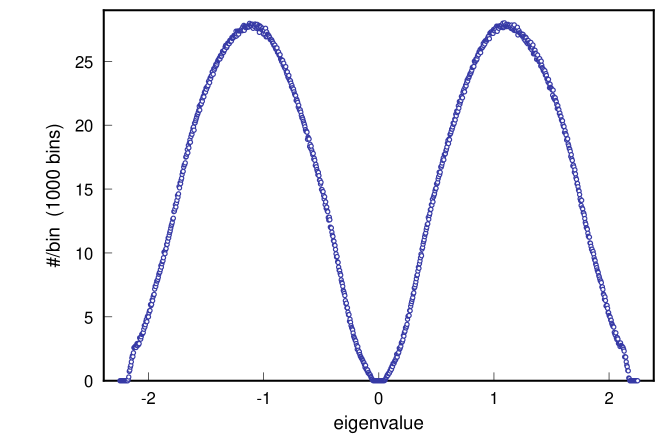
Figure 16: Spectrum of eigenvalues for $6^{4}$ lattice,$\beta$=5.7,$\kappa$=0.1685, $N_{\lambda}$=30

We can see the importance of the higher eigenvalues by separating the high and low part of the fermion determinant for each configuration. This is shown in Fig. 17. Unlike the case of QED2 (cf. Fig 1) it is apparent that the UV contribution to the determinant definitely involves large fluctuations. Of course, the issue here is just whether these fluctuations are well described by a simple effective gauge action.

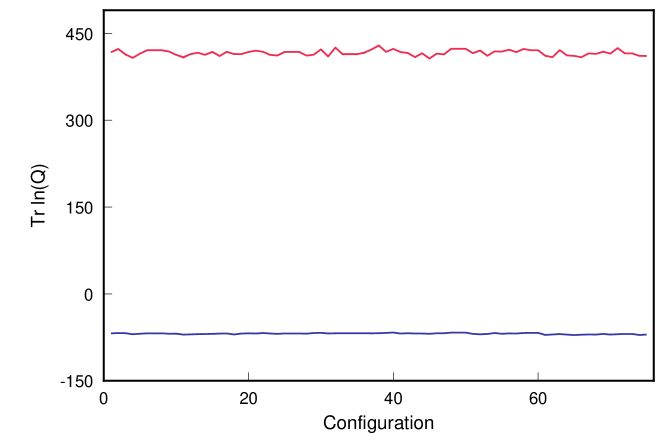
Figure 17: Fluctuations in the low ($n<30$) and high eigenvalues for the same configurations as previous figure.

Considering only the high eigenvalues, an excellent fit to the fluctuations is obtained including four and six link closed loops. The variance of the fit is 0.265. The comparison between the fluctuations in the exact and approximate actions for the high eigenvalue piece is shown in Fig 18.

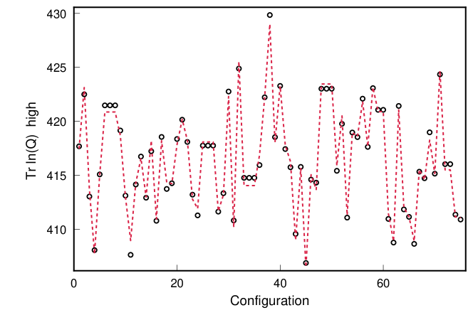
Figure 18: Fluctuations in the high eigenvalue piece of ${\rm Tr}\ln H$ are indicated by a dashed line. Fluctuations in the fitted effective gauge action (6 links and less) are indicated with open circles

As expected, if only the plaquette term is included the variance is larger (2.25) and we must move the low eigenvalue cutoff to $N=50$ ($\approx$ 700 MeV) to reduce the variance below one. The results for various cutoffs and terms included are shown in Table 1.

$n_{\lambda}$ cut	$\lambda$ (MeV)	4 link fit	6 link fit	6 link fit
			wo WL	with WL
0	0	4.98	1.074	0.835
$\pm 15$	340	2.25	0.2652	0.233
$\pm 50$	700	0.940	0.0564	0.0491
$\pm 250$	1,210	0.0733	0.0695	0.0641
$\pm 1250$	2,220	0.138	0.0198	0.0180

Table 1: Fits to the high eigenvalues of the quark determinant by various small gauge loops (WL denotes a Wilson line passing through the entire lattice).

Although more study is required this second method looks very attractive for dealing with the high end of the fermion determinant in full QCD with light dynamical quarks. Simulations would be performed by including the predetermined effective gauge action $S_{a}$ in the gauge updates and computing the infrared part of the determinant as in the truncated determinant simulations described in this paper.

In summary, we have found that there are at least two viable methods to deal with the contribution of the fermion determinant not computed explicitly in a truncated determinant approach.

7 Conclusions

We have proposed an algorithm for Monte Carlo simulation of full QCD with light dynamical quarks which has as its central feature a separation of the quark determinant into products over low and high eigenvalues. This separation is a direct reflection of the different physical roles played by these two sectors, with high eigenvalues (small quark loops) having the primary effect of modifying the gauge interaction strength, while the low eigenvalues (large quark loops) determine the long-range chiral structure of the theory. Our procedure for generating full QCD configurations then entails an exact calculation of some fixed number of the lowest lying eigenvalues of $H\equiv\gamma_{5}(D\!\!\!/(A)-m)$, using a Lanczos algorithm. This careful treatment of low Dirac eigenmodes is motivated by the conviction that the most essential differences between quenched and full QCD reside in their long-range chiral structure and associated topological properties.

The complete formulation of our proposed algorithm also allows various methods of incorporating the higher eigenvalues which were omitted in the Lanczos calculation. For example, the algorithm matches cleanly onto the multiboson approach. We have also explored a particularly promising approach for incorporating the correct ultraviolet behavior by the use of a sum over relatively small Wilson loops to represent the high-eigenvalue contribution to $\ln{\rm Det}\;H$. By doing a complete diagonalization on $6^{4}$ gauge lattices, we found that this Wilson loop representation works well with only a few small Wilson loops (4-link and 6-link) included. Here, the small loop approximation to the truncated $\ln{\rm Det}\;H$ only succeeds when the lowest eigenvalues ($<$300-400 MeV) are excluded, so it forms an ideal complement to the Lanczos treatment of the low eigenvalues. In the Monte Carlo simulations discussed in this paper, we have used the pure Wilson plaquette gauge action for the heat-bath sweeps and carried out the accept-reject test using the truncated low-eigenvalue contribution to the determinant. In the context of the more general Wilson-loop description of the high-eigenvalue segment, our present procedure is equivalent to approximating the high-eigenvalue contribution to $\ln{\rm Det}\;H$ by just the sum of a constant and a plaquette term. (This is in the same sense that the ordinary quenched approximation is equivalent to approximating the full determinant by a shift of $\beta$.)

Perhaps the best news to emerge from these numerical simulations is that the Metropolis test on the low-eigenvalue-truncated determinant yields a reasonably large acceptance ratio after one or more complete heat bath sweeps, even when the quarks are very light. This is in marked contrast to what would happen if one tried to include the full determinant via an accept-reject step between quenched Monte Carlo sweeps. Even for a single heat bath sweep, the fluctuations of the full determinant are much too large to yield a reasonable acceptance rate. The Lanczos calculation of the lowest few hundred eigenvalues requires an amount of computing time of the same order as that of an ordinary conjugate-gradient inversion of the Dirac operator. Thus, even if the accept-reject step is performed after every sweep, the computing required is still comparable to that of other full QCD algorithms such as hybrid Monte Carlo. Moreover, the performance of the algorithm does not seriously degrade in the light quark limit, which may provide a significant advantage over hybrid Monte Carlo for the study of chiral behavior in full QCD. Finally, for issues associated with chiral symmetry, the special handling of low eigenvalues is theoretically appropriate, and the eigenmodes extracted by the Lanczos analysis provide a detailed view of the connection between chiral symmetry breaking and the low-lying Dirac spectrum.

Acknowledgements

A. Duncan is grateful for the hospitality of the Fermilab Theory Group, where this work was performed. The work of A. Duncan was supported in part by NSF grant PHY97-22097. The work of E. Eichten was performed at the Fermi National Accelerator Laboratory, which is operated by University Research Association, Inc., under contract DE-AC02-76CHO3000. The work of H. Thacker was supported in part by the Department of Energy under grant DE-AS05-89ER40518. Much of the numerical work was performed on the Fermilab ACPMAPS system.

References

- [1] W. Bardeen, A. Duncan, E. Eichten, G. Hockney and H. Thacker Phys. Rev. (1998).
- [2] W. Bardeen, A. Duncan, E. Eichten, and H. Thacker, Phys. Rev. (1998).
- [3] W. Bardeen, A. Duncan, E. Eichten, and H. Thacker, hep-lat 9806002.
- [4] “The Uses of Instantons”, in The Aspects of Symmetry, Selected Erice Lectures of S. Coleman, (Cambridge 1985).
- [5] R. Setoodeh, C.T.H. Davies, and I.M. Barbour, Phys. Lett B213 195 (1988); K.M. Bitar, A.D. Kennedy, and P. Rossi, Phys. Lett. B234 333 (1990).
- [6] H. Leutwyler and A. Smilga, Phys. Rev. D46, 5607 (1992).
- [7] R. Narayanan and H. Neuberger, Nucl. Phys. B443 305 (1995).
- [8] A. Morel, J. Phys (paris) 48,(1987)1111; S. Sharpe, Phys. Rev. D41, (1990) 3233; C. Bernard and M. Golterman, Phys. Rev. D46 (1992)853.
- [9] M. Lüscher, Nucl. Phys. B418, 637 (1994).
- [10] J. Smit and J. Vink, Nucl. Phys. B286(1987)485; J. Vink, Nucl. Phys. B307(1988)549.
- [11] A. Duncan (speaker), W. Bardeen, E. Eichten, and H. Thacker, talk given at Lattice 97 (Edinburgh), in Nucl. Phys. Proc. Suppl. 63, 811 (1998).
- [12] T. Kalkreuter and H. Simma, Comput.Phys.Commun. 93 33 (1996).
- [13] G.H. Golub and C.F. Loan, Matrix Computations, 2nd edition (Johns Hopkins, 1990).
- [14] J. Cullum and R.A. Willoughby, J. Comp. Phys. 44 329 (1981).
- [15] T. Kalkreuter, Comput.Phys.Commun. 95 1 (1996).
- [16] A. Duncan, E. Eichten, J. Flynn, B. Hill, G. Hockney, and H. Thacker, Phys. Rev. D51 5101 (1995).
- [17] T. deGrand and A. Hasenfratz, Phys. Rev. D49 466 (1994).
- [18] W.H. Press, S.A. Teukolsky, W.T. Vetterling and B.P. Flannery, Numerical Recipes in C, 2nd ed. (Cambridge University Press 1992).
- [19] J. C. Sexton and D. H. Weingarten, Phys. Rev. D55 4025 (1997).
- [20] A. C. Irving and J. C. Sexton, Phys. Rev. D55 5456 (1997); A.C. Irving, J.C. Sexton and E. Cahill,hep-lat/9708004.
- [21] M. Lüscher and P. Weisz, Phys. Lett. 158B 250 (1985), and references therein.