Statistical analysis and the equivalent of a Thouless energy in lattice QCD Dirac spectra
Abstract
Random Matrix Theory (RMT) is a powerful statistical tool to model spectral fluctuations. This approach has also found fruitful application in Quantum Chromodynamics (QCD). Importantly, RMT provides very efficient means to separate different scales in the spectral fluctuations. We try to identify the equivalent of a Thouless energy in complete spectra of the QCD Dirac operator for staggered fermions from SU(2) lattice gauge theory for different lattice size and gauge couplings. We focus on the bulk of the spectrum. In disordered systems, the Thouless energy sets the universal scale for which RMT applies. This relates to recent theoretical studies which suggest a strong analogy between QCD and disordered systems. The wealth of data allows us to analyze several statistical measures in the bulk of the spectrum with high quality. We find deviations which allows us to give an estimate for this universal scale. Other deviations than these are seen whose possible origin is discussed. Moreover, we work out higher order correlators as well, in particular three–point correlation functions.
pacs:
PACS numbers: 11.30.Rd, 05.50.+q, 64.60.Cn, 12.38.GcI Introduction
It is now well established that Random Matrix Theory (RMT) accurately models spectral fluctuations in an abundant variety of different systems, such as chaotic, disordered and many–body systems, see the review in Ref. [1]. In recent years, RMT has in addition been successfully introduced into the study of certain aspects of Quantum Chromodynamics (QCD). The interest focuses on the spectral properties of the Euclidean Dirac operator. The eigenvalue equation under consideration reads
| (1) |
where is the massless Euclidean Dirac operator. The coupling constant is denoted by and the are the generators of the gauge group. The distribution of the color gauge fields is given by the Euclidean QCD partition function. As these gauge fields vary over the ensemble of gauge field configurations, the eigenvalues fluctuate about their average positions. The average spectral density is defined as
| (2) |
The average has to be performed over all gauge field configurations.
In contrast to most other systems, however, there are two different regimes in QCD spectra which can be addressed in an RMT approach, the microscopic region and the bulk region. Since the Dirac operator only couples states of opposite chirality, the eigenvalues are pairwise positive and negative. This is the reason why two types of spectral fluctuations can be distinguished, namely spectral fluctuations in the microscopic limit near zero virtuality, , and in the bulk of the spectrum.
Concerning the microscopic region, chiral Random Matrix Theory (chRMT) [2] incorporates the global symmetry properties, in particular chiral symmetry, of . It predicts level repulsion between positive and negative eigenvalues which results in a distinct behavior of the eigenvalue density and correlations near the origin. It is possible to calculate spectral correlators analytically in the microscopic limit [3, 4, 5], and to compare the predictions of chRMT with complete spectra of the lattice QCD Dirac operator on reasonably large lattices. Indeed, remarkable agreement is found [6, 7, 8, 9, 10] at the edge of the spectrum.
Sufficiently far away from the origin, however, the repulsion of negative and positive eigenvalues should become unimportant. Therefore the chiral structure of the theory is not expected to be of relevance in the bulk of the spectrum. This is the region we will address on in this work. By comparing with lattice data, it has already been shown that conventional RMT properly models these fluctuations in the bulk [11, 12, 10]. It is important to go beyond these statistical analyses made so far in order to see to what scales RMT does apply. The identification of such scales gives a fundamental insight into a system. Investigations of this type have been performed in great detail in disordered systems and in many–body systems. There, the Thouless energy or the spreading width determine the scale where is the level spacing, in which the fluctuation are of RMT type [13, 14]. Beyond this scale, deviations from the RMT behavior occur, see Ref.[1] for a detailed discussion and further references.
Recently, theoretical studies [15, 16, 17] established a link between disordered systems and QCD. The range of validity of RMT, , was introduced as an equivalent of a Thouless energy . A scaling was proposed where is the four–volume of the system. Indeed, such a scaling behavior was found very recently in the microscopic region [18] for deviation from RMT behavior. As argued in [16] a corresponding effect should also be seen in the bulk of the spectrum. This is what we will investigate.
The identification of this scale in QCD spectra could lead to an improved understanding of certain features of QCD and allows us to separate the stochastic noise of the short range fluctuations from the true dynamics of the QCD vacuum. Eventually, it could be possible to set up effective models or simplify the presently used simulation algorithms in lattice gauge theories. In this work, we search for such a universal scale in the bulk region by analyzing lattice data. In contrast to the microscopic region, the bulk of the spectrum is expected to have a translation invariant analogue of the Thouless energy. We emphasize that our analysis is self–consistent. Advantageously, it does not depend on any model that aims at an explanation for the occurrence of this universal scale.
The high amount and quality of the data sets which exceed the existing ones by far enable us to considerably extend the energy range for our analysis. Moreover, the wealth of data makes it possible to directly address bare correlation functions which cannot be analyzed in most systems. Furthermore, in doing so we discuss some technical aspects, which are of general interest for the investigation of spectral fluctuations.
This paper is organized as follows: In Sec. II the data under investigation is presented. A detailed analysis of the statistical properties is given in Sec. III. This includes the introduction of the numerical unfolding approaches, a statistical analysis of the nearest neighbor spacing distribution, two–point spectral correlations and higher order spectral correlations. Deviations from the RMT predictions are found and interpreted. Summary and discussion are given in Sec. IV.
II Complete Dirac spectra in SU(2) gauge theory
The computation of large ensembles of complete spectra of the Euclidean Dirac operator for staggered fermions in SU(2) gauge theory has recently been performed Ref.[19] expanding the numerical work of [20]. In lattice gauge theory simulations one generates a sequence of gauge field configurations distributed according to the Boltzmann weight. On each of the gauge field configurations the eigenvalue equation (1) is solved numerically on the lattice and a distinct partition of eigenvalues is obtained. The lattices have the size where denotes the length of the Euclidean box with a lattice spacing . Parameters and statistics of the simulation are summarized in TableI. The choice of SU(2) as the gauge group implies that every eigenvalue of is twofold degenerate due to a global charge conjugation symmetry. The random–matrix ensemble for this situation has symplectic symmetry and is referred to as chiral Gaussian Symplectic Ensemble (chGSE) [21, 1]. In addition, the squared Dirac operator couples only even to even and odd to odd lattice sites, respectively. Thus, has distinct eigenvalues. We use the Cullum–Willoughby version of the Lanczos algorithm [22] to compute the complete eigenvalue spectrum of the sparse hermitian matrix in order to avoid numerical uncertainties for the low-lying eigenvalues. There exists an analytical sum rule, , for the distinct eigenvalues of [20]. We have checked that this sum rule is satisfied by our data, the largest relative deviation was about .
Examples of the spectra are shown in Fig. 1, where the average level density and the integrated average level density, see Eq. (3), for a , i.e. , lattice are shown. It should be pointed out that due to the distinct eigenvalues of each configuration there are millions of eigenvalues at our disposal. We used two different values of the gauge coupling where the weak coupling regime of SU(2) sets in and where most of the scaling test have been performed so far. Finally, the chiral condensate was obtained by fitting the spectral density and extracting . Our findings [19] are in rough agreement with the values obtained by Hands and Teper [23] for the same simulation parameters in SU(2) but only the 20 smallest eigenvalues have been computed by these authors.
III Data analysis
In this section we give a detailed analysis of the data introduced in the previous section in the bulk of the spectrum. We start with a description of the numerical unfolding approaches and their properties in Sec. III A. After a short discussion of the nearest neighbor distribution in Sec. III B, we present data for spectral two–point correlations at large scales in Sec. III C. From this we identify the equivalent of a Thouless energy. Furthermore we discuss higher order correlators, in particular three–point correlations in Sec. III D. A qualitative explanation of deviations from RMT predictions which are not due to the Thouless energy is given in Sec. III E.
A Unfolding
As RMT is capable of making predictions for the fluctuations on the scale of the mean level spacing, one has to remove the influence of the level density by unfolding the spectra. The cumulative spectral function
| (3) |
is the number of levels below or at the energy . It is frequently referred to as staircase function. It can be separated into an average part , whose derivative is the level density, and a fluctuating part ,
| (4) |
The average part is determined by gross features of the system and has to be removed. The fluctuating part is in all relevant systems of order and contains the correlations to be analyzed. After extraction of the average part , it is unfolded from the spectra by the introduction of a dimensionless energy variable
| (5) |
In this variable, the spectra have mean level spacing unity everywhere,
| (6) |
where . However, the extraction of from the data is non–trivial in our case because little is known analytically about the level density of QCD spectra, particularly in lattice calculations. We thus have to resort to phenomenological unfolding procedures. Faulty unfolding leads to wrong results, especially on such large energy scales that we are interested in. In the subsequent Secs. III A 1, III A 2 and III A 3, we discuss three different procedures used here, ensemble unfolding, configuration unfolding and windowing, respectively.
1 Ensemble unfolding
In RMT one deals with an ensemble of matrices, where the matrix elements of each member are chosen randomly. Spectral observables predicted by RMT are calculated as an average over the ensemble. This ensemble average is denoted by a bar . But observables can also be calculated as spectral average, i.e. one performs a running average over overlapping intervals of length in the spectrum of one member. In order to distinguish it from ensemble average, we denote spectral averaging by angular brackets . In the limit of large matrix dimension both averages are equivalent [1]. This property is called ergodicity.
In most experiments, one measures one - preferably long - spectrum. Thus observables are usually calculated from spectral average. One uses the theoretical concept of ergodicity to compare the RMT predictions with the experimental results. In our case, however, the data consists of configurations, i.e. forms an ensemble. Hence, questions related to ergodicity arise not only for the calculation of observables, but also in the determination of the staircase function, i.e. in the unfolding procedure. We have in principle two very different ways of unfolding our data: first, ensemble unfolding, , i.e. we determine the smooth part of the staircase function by averaging over the ensemble, and second, configuration unfolding, , i.e. we determine the smooth part of the staircase function for every configuration separately. The results differ considerably, , for most of the configurations. The ensemble averaged staircase for the lattice QCD Dirac operator is shown in Fig. 1. We find by dividing the energy range in bins with width and average the density for each bin over all configurations. We then calculate the staircase function as , with . In Fig. 2, the difference between the ensemble averaged staircase function and the configuration wise averaged ones, for and , for 50 arbitrarily chosen configurations is plotted. Each data point represents the difference , where enumerates the eigenvalues, and is the configuration number . We plot only every 500th eigenvalue. There are deviations of about in certain energy ranges.
If the spectra are unfolded using the ensemble averaged staircase function , observables should then also be calculated as an ensemble average for a fixed value of . But we checked that our results do not depend on in a wide range of the bulk. This property is called translational invariance. It is actually not present in the microscopic region, where it is destroyed by point wise symmetry between positive and negative eigenvalues [18]. Translational invariance in the bulk allows us to calculate observables from running average over overlapping intervals for each configuration. We choose an overlap of for two consecutive intervals. Then we average over all configurations. This improves the statistics of the result considerably.
2 Configuration unfolding
We now unfold each configuration separately. Observables are then calculated for each configuration by running spectral average. Thereafter we average over the ensemble. The basic characteristics are already obtained for one single configuration, though the statistics is considerably improved by ensemble averaging. This is in the same spirit as it was done in spectra of nuclei [24] and complex atoms [25]. These spectra were unfolded for each nuclei or atom separately. Then observables were calculated as described above, i.e. first taking the spectral and then the ensemble average. In this case the ensembles consist of nuclei or atoms of different types.
Configuration unfolding is, in contrast to ensemble unfolding, not a unique procedure. One has to find either fits to the average staircase function or to smooth it in some way. A priori, there is no criterion whether the numerical estimated is close to the real one or not. Thus, we use three different approaches and carefully compare them with one another to eliminate as many sources for mistakes as possible and to obtain consistent results.
First, we fit to a polynomial of degree ,
| (7) |
where is a small integer, . This approach is motivated by the fact that almost all physical systems are known to have a level density which is as smooth as a polynomial. In our case this ansatz is supported by pertubative calculations. Strong coupling expansions for SU(2) with staggered fermions have been performed [26] and, furthermore, expansion of the QCD level density [27], both suggesting a smooth level density. The former gives a semi–circle whereas the latter explicitly predicts a polynomial increase.
Second, we use the Gaussian method which was originally developed by Strutinsky [28]. One replaces the –functions in Eq. (3) by Gaussian functions with a width which yields a smoothed staircase
| (8) |
The summation runs from the smallest eigenvalue to the largest eigenvalue in the interval under consideration. The limit restores –distributed eigenvalues, whereas the fluctuations are smeared out for finite . The optimal parameter is found by a –fit of to . Then we identify
| (9) |
Third, we perform a local unfolding by calculating the unfolded eigenvalues directly with the formula
| (10) |
with local mean level spacing
| (11) |
Here is the number of consecutive level spacings over the running average is performed.
Whatever approach one decides to use, a necessary condition is that on the unfolded scale the average number of levels in an interval of length should equal this length. This is a very important requirement because we are also interested in very large energy scales. This assures that the spectrum on the numerically constructed dimensionless scale has mean level density unity. Consider the interval which contains eigenvalues. Spectral average and ensemble average have to yield
| (12) |
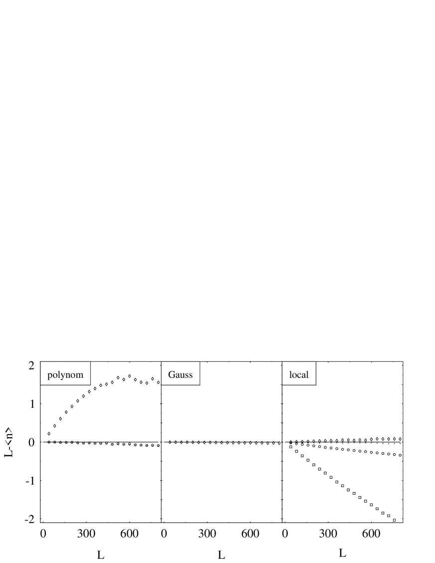
In Fig. 3, the difference between the calculated mean number of eigenvalues and is plotted as a function of . For the Gaussian method the difference appears to be zero to all scales. While it is small and does only appear at large for polynomials fits with , strong deviations from the zero line already appear at small for . In the case of local unfolding, the difference is positive for small , i.e. there are on average less levels in a given interval than there should be. For growing , it becomes negative with ever stronger deviations from the flat line. The averaging interval length for which the difference equals zero is for . For other lattice sizes this averaging interval is slightly smaller. We take this as the optimal parameter for this approach. From Fig. 3 we learn, that the necessary condition (12) is fulfilled only for the Gaussian approach, polynomial fit with and local unfolding with for , all other choices of the parameters must be rejected.
It should be mentioned that a new artificial scale both for local and Gaussian approach is introduced, namely the averaging interval length and the width , respectively. Therefore, one should be cautious in the interpretation of effects seen on scales larger than current value of the corresponding parameter. In units of the mean level spacing we find a width of the Gaussian as at a lattice. On the other hand, both approaches have the advantage that no particular function for the average level density has to be assumed.
We checked all our numerical unfolding approaches with the spectrum of a very different system. We used the spectrum of quantum chaotic billiard that was simulated in a microwave experiment. In billiards, the Weyl formula gives an analytically expression for the mean level density [29]. With our phenomenological approaches, we indeed obtained quantitatively the same results.
3 Windowing
Ideally, an unfolding procedure should only remove the global variations of the spectral density, i.e. in our case the overall behavior seen in Fig. 1. For reasons which will become clearer later, it is difficult to numerically distinguish the global variations from the local fluctuations. This is in particular the case for data of large lattice size. In other words, we might have removed too much by some of the unfolding procedures, while we might have removed too little by others. This will be discussed in great detail below, especially in Sec. III E.
One has to ensure that any deviations seen in the spectral statistics are not due to global variations in the average density which were not removed adequately. One way is to use different unfolding approaches and compare the results carefully. Another way is to take only a small window of the spectra in which the global variation of the density is expected to be small. Thus we choose an interval and calculate the ensemble averaged mean level spacing for it. We then rescale the eigenvalues in this interval as
| (13) |
This is done in the same manner as in [8] where the microscopic region was considered. However, it is not clear beforehand that a scale in the spectra, if any, does not exceed the interval length . Unfolding, if done correctly, allows to make investigations to much larger scales.
This approach is closely related to ensemble unfolding defined above. Indeed, the results coincide, but with a less statistical significance by only rescaling. By using this approach, we intended to avoid any unfolding procedures. As we will see later, there are a slight, but still systematic variations of the spectral density within the small window.
B Nearest Neighbor Spacing Distribution
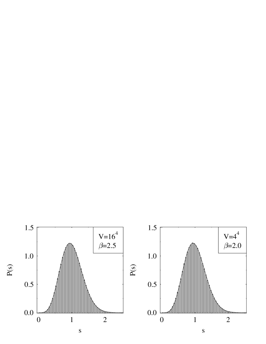
The nearest neighbor spacing distribution probes the fluctuations on short scales in the spectra. It is the probability of finding the distance between adjacent level on the unfolded scale. It contains all correlations of order . In the case of completely uncorrelated levels which is referred to as Poisson regularity [1], it is given by . In the case of GSE type correlations, Wigner surmized the shape
| (14) |
which is very close to the exact GSE result. As shown in Fig. 4, the data is in perfect agreement with the prediction. This is as well true for the large lattice, (left part), as for the small lattice, (right part). The spacing distribution of the intermediate lattice sizes are not distinguishable from the both shown. We have complete agreement between theory and lattice data for any choice of lattice size and coupling constant.
C Two–Point Spectral Correlations
In an interval of length in units of the mean level spacing, the mean number of eigenvalues should be equal to , see Eq. (12). The variance of this number is defined by [30]
| (15) |
Thus, an interval of length contains on average levels. For uncorrelated Poisson spectra . RMT predicts for the number variance stronger correlations, namely .
Another important quantity is the spectral rigidity , defined as the least square deviation of the staircase function from the straight line [30],
| (16) |
Since it can be expressed as an integral over the number variance
| (17) |
it is smoother than .
The number variance can be expressed as an integral of the two–point cluster function [30], which depends for translational invariant spectra only on the difference between two levels at and ,
| (18) |
The cluster function is related to the two–point correlation function which measures the probability density to find two levels at a distant by . In contrast to , these two levels are not restricted to adjacent ones.
In Fig. 5, number variance and spectral rigidity for scales up to and , respectively, are shown. Lattice data and RMT predictions agree remarkably well, even the oscillations in are accurately reproduced. Naturally, previous analyses [11] with smaller data sets have less statistical significance. Two–point cluster and correlation function which usually are not accessible in data analysis are shown in Fig. 6. Again, the agreement is impressive.
Beyond this scale there are considerable deviations of as well as of from RMT predictions which depend on the unfolding procedure used. We mention that on general grounds one can show that any scales in and , say and , respectively, are related by , or so [1], see Fig. 5. Thus, any deviations from RMT behavior appear at smaller in as compared to .
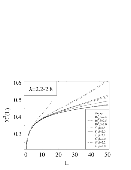
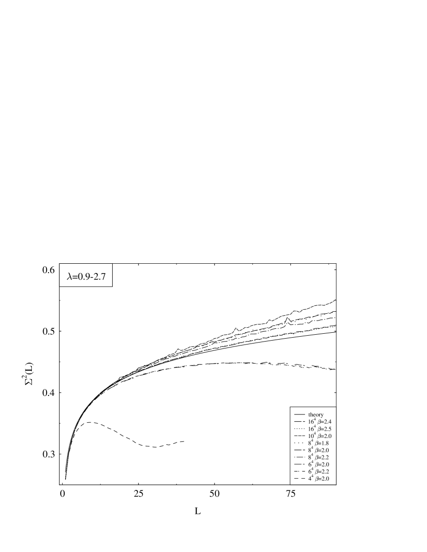
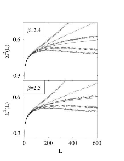
If we unfold with the ensemble staircase function , we obtain the following results. The number variance can be seen in Fig. 7. Data for different lattice sizes and different gauge couplings are shown in comparison to the RMT predictions for some regions of the spectra. We find that the point where the deviation sets in, scales with the square root of the lattice volume,
| (19) |
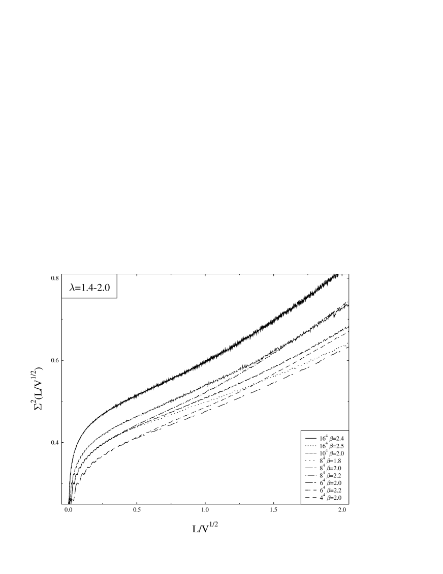
The numerical constant is approximately given by . This should be compared with the result obtained in [18] for the microscopic region. There, the scaling was found. This is independent of the region of the spectra we consider and of the coupling strength . This is shown in Fig. 7. There different regions of the spectra are considered, each corresponding to different values of , see Fig. 1. The results are the same. Furthermore, the deviation points for different appear to coincide, whereas the local average density depends on the gauge coupling, , see Fig. 1. The scaling relation (19) can nicely be seen from Fig. 8, in which the axes of Fig. 7 is rescaled with . We see that the crossover from RMT to non–universal behavior appears to be the same for all lattice sizes independent of . But the slope varies for different couplings and regions of the spectra. When we use windowing instead, we get the same results as obtained by ensemble unfolding. But the data points scatter more compared to Figs. 7 and 8.
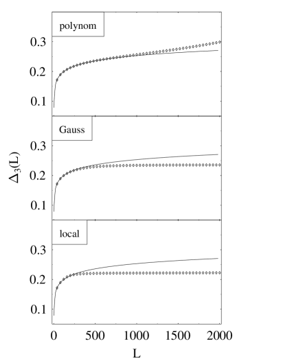
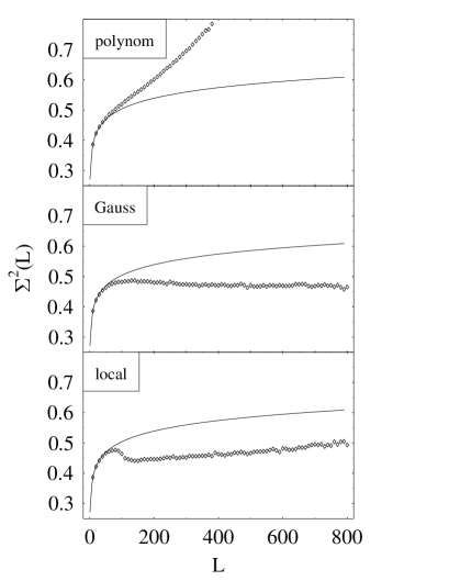
The importance of a proper choice of the unfolding method becomes manifest as the above picture changes drastically if we unfold each configuration separately. As displayed in Fig. 9, the polynomial unfolding leads to an overshooting of the data over the predictions but further out, compared to ensemble unfolding, while in the Gaussian as well as in the local case saturates. Note the different scale compared to Fig. 7 and also the difference in scale between number variance and spectral rigidity, as mentioned above. The result of the polynomial approach does not depend on the degree of the polynomial. Furthermore we find no scaling with for the deviations of polynomial unfolding, see Fig. 10. The deviation point appears to be the same for different lattice sizes. The saturation of the small lattices is due to the limited number of eigenvalues in the considered energy range. The same picture arises for the number variance: overshooting for the polynomial, saturation for Gaussian and local approach. The general tendency of this results are already obtained for each configuration separately, but the data points scatter. After averaging over all configurations the scattering becomes much smaller, see Figs. 5 and 9.
D Higher Order Spectral Correlations
The wealth of data allows us to go beyond a previous analysis [12] of higher moments of the eigenvalue partition,
| (20) |
We notice that . The skewness and the excess [30] are defined by
| (21) |
and
| (22) |
respectively. The comparison of RMT predictions with lattice data for these both quantities in Fig. 11 again shows very good agreement.
The measures and only contain a small amount of information of the spectral correlations. Moreover, and also involve lower order correlations: is a combination of the two– and the three–point correlator, and , and involves in addition the four–point correlator . The representation of the moments in terms of integrals over the correlators reads
| (23) |
and
| (24) | |||||
| (25) | |||||
| (26) |
Obviously, by analyzing and , one cannot easily estimate to what extent the three– and the four–point correlators themselves obtained from the lattice calculations follow the predictions of RMT.
Here, the three– and the four–point cluster functions, and are written as functions of the arguments () which are defined terms of the original arguments () by
| (28) |
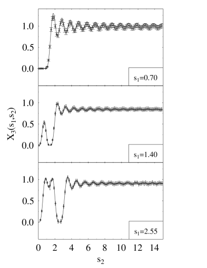
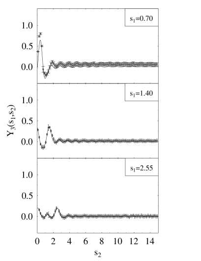
We constructed from the data the two–point and the three–point correlation functions and and the corresponding cluster functions and . Here, for convenience, we redefined the arguments for the three–point correlators as follows:
| (29) |
The results for and are plotted with error bars in Fig. 12 for some given values of . The results do not depend on unfolding. In the construction of these correlators, we first performed a spectral average by using the translational invariance due to unfolding, and then averaged over the ensemble. The errors for and were estimated as the variance of the ensemble fluctuations. Once more, very good agreement with the RMT predictions for is found, apart from a small systematic deviation which we believe can be understood as follows. From the relation between and
| (30) |
one has
| (31) |
Therefore, even a small point–deviation of the two–point correlator at from the theoretical predictions can result in a systematic deviation of the whole curve versus for this given . For , the quality of the agreement with RMT is only slightly reduced, but still remarkable. In addition to the systematic deviation, one can see some random fluctuations around the theoretical curves. This is because is the disconnected correlator, and it should represent the true three–point correlation, while also contains the two– and one–point functions. They play a dominate role and are in good agreement with the corresponding GSE predictions. We notice that this analysis was only possible due to the extremely higher number of levels available.
E Qualitative discussion of the deviations for configuration unfolding
Using ensemble unfolding, we find deviations from RMT behavior, which scale with the square root of the volume according to the theoretical predictions. But as we unfold each configuration separately this effect vanishes. There are still deviations left but none of them show a scaling law. Moreover, we have a dependence of the results on the unfolding approach.
Concerning local and Gaussian unfolding, an explanation seems to be easy at hand. As mentioned above, both procedures have an intrinsic, artificial, scale. In units of the mean level spacing it has the value for in both cases. This is approximately where the saturation of the statistics seen in Fig. 9 sets in. We conclude that this artificial scale causes and to saturate. In other words, both approaches are not capable to allow statements at scales . Nevertheless, both approaches do not show a behavior as shown in Figs. 7,8 for .
On the other hand, the polynomial unfolding also deviates from RMT predictions, see Fig. 10. As this approach does not contain an additional scale, we can rule out effects like the one discussed above. The question is, whether the deviations in Fig. 10 are due to a Thouless energy or if they have another origin.
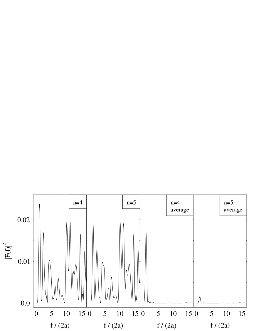
The fluctuating part of the integrated level density should be of order , as mentioned above. In the upper part of Fig. 13 the difference between the real staircase function and the smooth polynomial staircase function, , for one specific configuration is plotted. This picture remains qualitatively the same whatever configuration is chosen. The polynomial fits have a systematic deviation from a smooth behavior larger than . The difference between the ensemble staircase and polynomial fit is shown in the lower part of Fig. 13. A polynomial of degree gives the same result as . To obtain a better insight in this obviously not universal behavior, we calculate the power spectrum
| (32) |
By construction, the derivative in the integrand gives the fluctuations of the level density. The window function has to be introduced because we only have a finite interval of eigenvalues in the Fourier transform over the whole real axis. It is zero outside the interval . The choice is not unique inside [31]. Thus, the Fourier transform is a convolution of the transforms of and . In order to reduce the influence of the Fourier transform of on the results as far as possible, we use a triangle window [31]. The result is shown in Fig. 14. In the right part one sees the Fourier transform of the ensemble averaged density. Only the very first peak is left, both for polynomial of degree and . The latter is reduced in amplitude. On the left side the transform of an arbitrary chosen configuration is plotted. The first peaks are reduced in amplitude again for , whereas the remaining ones are the same for both degrees. We conclude that only the first peak, corresponding to the long wave part of Fig. 13, is common to all configurations. All others fluctuate from configuration to configuration.
We conclude that the average level density and thus the average integrated level density consist of two parts, namely a very smooth polynomial–like part and another, non–universal, part,
| (33) |
We stress again that the existence of a polynomial–like smooth part is suggested by pertubative and expansions of the QCD level density [26, 27]. It is expected to be governed by the available phase space: for free fermions the spectral density is given at by [32], where is the number of colors. This also holds in a expansion of the interacting theory on scales which are large compared to the hadronic scale [27]. This is the region we investigated in the spectra, as the eigenvalues are given in units of the inverse lattice spacing as , see Figs. 1 and 13. This is why we tried to approximate the average level density by a function which is as smooth as a polynomial.
The additional structure of the level density appears to have similarities to oscillations, see Figs. 13 and 14. Thus, we refer to it as “oscillatory part”, . This oscillatory part explains the different behavior of and for large for different unfolding methods. The polynomial unfolding is clearly unable to remove the oscillations and fits only . Thus, the oscillatory part is still present in the unfolded spectrum. The presence of these oscillations leads to values for larger than predicted by RMT, because a fit to a straight line can only be done in a less accurate manner. In contrast to that, the Gaussian and the local unfolding is capable to fit and part of . However, it is not clear whether the fit to the oscillatory part is done completely or if, on the other hand, it does not smooth out part of the universal fluctuations, i.e. overfits the data points. But, because of the saturation of and , see Fig. 9, we think that probably the latter happens.
However, as argued above, since we expect the physical density to be as smooth as a polynomial, the oscillatory part is likely to be a lattice artifact. This is suggested by Figs. 13 and 14 which show that these oscillations live on the scale of the inverse lattice spacing . As cannot be arbitrarily large in lattice gauge theory, due to an ultraviolet cutoff in momentum for finite lattice spacing , the increase of the density is disturbed by lattice artifacts. For the large lattices, i.e. , the deviations due to lattice artifacts set in at approximately the same scale as the expected equivalent of a Thouless energy. This can be seen from the scaling of the smaller lattices. A rough estimate gives for for . Therefore one should be careful with the determination of the deviation point for large lattices in the bulk of the spectra. After removing this part from the data, we find for reasonable agreement with the RMT prediction up to at least and with some uncertainties even to , see Fig. 15. Because of the complicated structure of the average level density it is not possible to make any statement beyond this scale. In chaotic billiards, so–called bouncing ball modes generate effects which are similar to the ones here [29]. In that case, however, an analytical prediction for the oscillatory behavior was at hand. Such a result is also highly desirable in our case. It would be needed to furnish our phenomenological removal of the oscillations with a theoretical justification.
In any case, we may use the information displayed in Fig. 14 to phenomenologically remove the oscillatory part. We cut the power spectrum at a certain interval, back transform the remaining peaks in the frequency interval and subtract the smooth oscillatory part of the integrated level density obtained in this manner. We do this for each configuration separately. This procedure changes the result of the statistical analysis in a crucial way, as can be seen from Fig. 15. There, the results for spectral measures are shown for different choices of . Because only the very first peak is common to all spectra whereas higher frequencies appear to be specific for each configuration, a choice of is actually too large. This manifests in a saturation of the statistics in Fig. 14 for . A cutoff of seems to be the best choice, but we are not able to give an exact value. This figure also shows a comparison between and for . Both values of give almost the same result. The procedure also removes the slight differences seen in Fig. 3 for the polynomials for . From all this, we conclude that the deviations in Fig. 10 are due to a non polynomial–like part in the average level density and not due to an equivalent a Thouless energy.
A possible way to circumvent the problems encountered by lattice artifacts is windowing as discussed in Sec. III A 3. However, this works only if the size of the windows is at least so small that the oscillations of Fig. 13 are not important, i.e. . Another way might be ensemble unfolding, Sec. III A 1. As the lattice artifacts are seen in each configuration as well as in the average integrated level density this approach might remove the oscillations. But it is by no means clear if it really does, especially for large interval lengths. As both approaches give similar results for small lattices, , for intervals , we conclude that the artifacts are not important on these scales. This is supported by the observations that deviations due to them set in at for polynomial unfolding, independently of the lattice size, see Fig. 10. Thus, these artifacts become important for analysis of larger lattices, i.e. , and for even larger ones in future examinations.
From all this we conclude that we do not see an equivalent of a Thouless energy if we unfold each configuration separately. This is in complete contrast to the results gained by ensemble unfolding. The former surely removes the fluctuations in Fig. 2, whereas the latter does not. We conclude that this fluctuation with respect to the ensemble already contains the information needed to determine the Thouless energy. After removing this information it seems that there is no further information in the spectra, i.e. we find agreement with RMT on huge scales.
IV Summary and discussion
A Summary
We presented a detailed analysis of statistical properties of complete eigenvalue spectra for staggered fermions for SU(2) lattice gauge theory for various couplings and lattice volumes. Unfolding the data posed certain difficulties which are not encountered in other systems. The staircase function found by an average over the ensemble differs in most cases from the smooth staircase of one specific configuration. The deviations are as large as for . Varying the unfolding approach leads to different results for large scales. In particular, there is a drastic difference between ensemble and configuration unfolding.
Using ensemble unfolding, we find a range of validity of RMT, giving . The numerical constant is approximately given as . which is compatible with the result obtained in [18] for the microscopic region where the scaling was found. The same results are obtained if we use windowing, but with less statistical significance.
By unfolding each configuration separately, we do not see any scaling of this type. This procedure obviously removes the fluctuations of the staircase function relative to the ensemble average seen in Fig. 2. We notice that fluctuations over the ensemble can already be observed in the integrated level density. But there are still deviations depending on the unfolding approach used. In particular there is an overshoot for polynomial unfolding at large . The reasons for this lies in special features of the average level density, which consists of at least two parts: a smooth polynomial–like and an oscillatory part. Hence the Thouless energy is due to the fluctuations in the ensemble.
We want to clarify the difference in the notion of ergodicity used in spectral analysis and in lattice calculations, respectively. Concerning the analysis of spectra, a system is called ergodic if spectral and ensemble average yield the same results. It can be proven rigorously that random matrices have this property in the limit of large matrix dimension. However, here we face a different situation. We emphasize that these issues do not affect the notion of ergodicity as used in connection with lattice simulations. The latter is defined by the requirement that the space of possible lattice configuration is explored reasonably fast by the simulation algorithm. We emphasize that the time history of the spectra is not of importance for the calculation of the spectral observable of Sec. III, because it is only relevant that the configurations used, see Table I, are representative members of the ensemble, i.e. ergodicity in the sense of lattice simulations is fulfilled. This is ensured by our algorithms as described in Sec. II. Furthermore, this is supported by the observation that our results do not change if we take arbitrary subsets of configurations, only the scattering of the data points increases.
Furthermore we analyzed the nearest neighbor–spacing distribution, skewness and excess for small . Due to the large amount of data, our results achieved a quality never reached before. Due to translational invariance in the bulk of the spectra the general tendency for all of the observables can already be seen for one specific configuration. Averaging over all configurations increases the statistical significance of the results. The results for small values considerably improve the statistical significance of previous analyses[11, 12]. To the best of our knowledge, we presented the first statistically highly significant analysis of bare two– and, importantly, three–point spectral correlators. Very good agreement between lattice data and RMT predictions is found. We find minor deviations for the three–point cluster functions. In our opinion, their origin are probably very small point–deviations of the two–point functions.
B Discussion
Some scenarios for the level statistics are shown in Fig. 16. There the spectral rigidity is plotted. The two solid lines represent Poisson and RMT behavior, and , respectively. The dashed lines represent schematically two different cases. Case ‘A’ correspond to a scenario known from systems with few degrees of freedom. The shortest periodic orbit in phase space sets a scale which forces to saturate at a certain [33]. But by increasing the degrees of freedom of the system, this scale become ever larger and is hard to be seen. As we may view lattice gauge theory as a many body problem or disordered system, we do not expect to see this scale in the level statistics. Therefore one should not be tempted to conclude that the saturation seen in Figs. 9,15 is the analogue of “saturation of fluctuation measures” which was observed in the energy level statistics for classically chaotic systems and was interpreted by Berry in terms of shortest periodic orbits [33]. Unlike in the case of quantum billiards where an analytic expression for the average spectral density exists, the that we obtained in our analysis was only a numerical result. Most likely all three approaches, i.e. Gauss, local and modified polynomial, fit also parts of the universal fluctuations which shows up as a saturation of the statistics and .
Another scenario is given by case ‘B’ which lies between Poisson and RMT behavior. It can arise in three different physical situations [1]:
-
1.
Systems in few degrees of freedom between regularity and chaos. The spectral rigidity lies between the Poisson limit, which applies to regular systems and the RMT limit which applies to chaotic systems, provided the scale is much larger than .
-
2.
Disordered systems in dimensions. The time for the classical diffusion through the system of size where is the size in each dimension determines an energy scale
(34) the Thouless energy. This in turn sets the scale where is the single particle mean level spacing. For energy separations in units of smaller than this scale, RMT fluctuations are seen. For larger energy separation, deviations as sketched in Fig. 16 occur.
-
3.
Many body systems such as nuclei, molecules or complex atoms. In the language of condensed matter physics, these systems are zero–dimensional. Consider the Hamiltonian of such a system where has a certain property and breaks this property. The influence of on the statistics of the spectrum of is measured in terms of the spreading width
(35) where is the mean level spacing of and the mean square matrix element of . In particular, if has Poisson statistics and RMT statistics the spectral rigidity acquires the form of Fig. 16 and sets the scale .
As discussed above, situation 1. is not likely to apply. We emphasize that the Thouless energy and the spreading width defined in 2. and 3. are closely related concepts. Actually, in his original paper, Thouless [13] defined as a special kind of spreading width. The precise relation between and has been studied in great detail in the framework of RMT [34]. We notice that the definition in 2. which is most commonly used in condensed matter physics, relates to dimensionality, whereas is defined in zero dimensions. Thus, the sheer existence of a scale can imply, but does not necessarily imply that the deviation from RMT is related to a diffusion in a dimensional disordered system.
Recent theoretical studies aim at establishing [15, 16, 17] a link between disordered systems and QCD. In these works, a range of validity of applicability of RMT was considered. Using the Gell-Mann-Oakes-Renner relation, it should be determined by the pion decay constant and the chiral condensate ,
| (36) |
In the microscopic region the mean level spacing is , so that Eq.(36) can be rewritten as
| (37) |
The predicted scaling behavior was found very recently in the microscopic region [18]. There a crossover from RMT to non–universal behavior was found with the scaling Eq.(37). As argued in Ref. [16], a similar relation should also be seen in the bulk of the spectrum. Here, however, the mean level spacing is that of the bulk. In the present work, we have shown that, first, the scale exists in the bulk, and, second, that it shows the predicted scaling behavior. The latter observation is a support for the ideas that link QCD to disordered systems and thus to a diffusion in a dimensions. However, as outlined above, our findings are necessary but not sufficient for this conclusion. They do not rule out other physical mechanisms that lead to a spreading width or Thouless energy. This underlines the strength of our analysis: it does not depend in any way on a model for this mechanism. It is a self–consistent statistical method to find the scale .
We hope that the identification of this scale can help to improve our understanding of certain features of QCD as it may allow one to separate the stochastic noise of the short range fluctuations from the true dynamics of the QCD vacuum. Most desirably, these results could help to design effective models or to simplify the presently used simulation algorithms in lattice gauge theories.
Acknowledgments
It is a pleasure to thank M.E. Berbenni-Bitsch for her help in generating the data sets. We are grateful to C. Mejia, H.J.Pirner, A. Schäfer, H.A. Weidenmüller and T. Wettig for enlightening discussions. We thank H.L. Harney and H. Alt for supplying the data set of Ref. [29] for test purposes. T.G. acknowledges support from the Heisenberg foundation. S.M. thanks the MPI für Kernphysik for the hospitality and acknowledges the support by a DFG grant Me 567/5-3 .
REFERENCES
- [1] T. Guhr, A. Müller-Groeling and H.A. Weidenmüller, Phys. Rep. 299, 189 (1998).
- [2] E.V. Shuryak and J.J.M. Verbaarschot, Nucl. Phys. A560 306, (1993).
- [3] J.J.M. Verbaarschot and I. Zahed, Phys. Rev. Lett. 70, 3852 (1993).
- [4] P.J. Forrester, Nucl. Phys. B402, 709 (1993).
- [5] T. Nagao and P.J. Forrester, Nucl. Phys. B435, 401 (1995).
- [6] M.E. Berbenni-Bitsch, S. Meyer, A. Schäfer, J.J.M. Verbaarschot and T. Wettig, Phys. Rev. Lett. 80, 1146 (1998).
- [7] M.E. Berbenni-Bitsch, A.D. Jackson, S. Meyer, A. Schäfer, J.J.M. Verbaarschot and T. Wettig, Nucl.Phys. B (Proc.Suppl.) 63, 820 (1998).
- [8] J.Z. Ma, T. Guhr, and T. Wettig, Eur. Phys. J. A 2, 87 (1998).
- [9] J.J.M. Verbaarschot, Phys.Lett. B 368, 137 (1996).
- [10] for a comprehensive review see J.J.M. Verbaarschot, hep-th/9710114.
- [11] M.A. Halasz and J.J.M. Verbaarschot, Phys. Rev. Lett. 74, 3920 (1995).
- [12] M.A. Halasz, T. Kalkreuter and J.J.M. Verbaarschot, Nucl. Phys. Proc. Suppl. 53, 266 (1997).
- [13] D.J. Thouless, J. Phys. C 8, 1803 (1975).
- [14] D.J. Thouless, Phys. Rev. Lett. 39, 1167 (1977).
- [15] J. Stern, hep-ph/9801282, submitted to Phys. Rev. Lett.
- [16] J.C. Osborn and J.J.M. Verbaarschot, Phys. Rev. Lett. 81, 268 (1998), Nucl. Phys. B525, 737 (1998).
- [17] R.A. Janik, M.A. Nowak, G. Papp and I. Zahed, Phys. Rev. Lett. 81, 264 (1998).
- [18] M.E. Berbenni-Bitsch, M. Göckeler, T. Guhr, A.D. Jackson, J.-Z. Ma, S.Meyer, A. Schäfer, H.A. Weidenmüller, T. Wettig and T. Wilke, Phys. Lett. B438, 14 (1998).
- [19] M.E. Berbenni-Bitsch, PhD Thesis, Universität Kaiserslautern, 1998.
- [20] T. Kalkreuter, Phys. Rev. D 51, 1305 (1995).
- [21] J.J.M. Verbaarschot, Phys. Rev. Lett. 72, 2531 (1994).
- [22] J. Stoer and R. Bulirsch, Introduction to Numerical Analysis (Springer (New York) 1993, 6.5.3.).
- [23] S.J. Hands and M. Teper, Nucl. Phys. B 347, 819 (1990).
- [24] O. Bohigas, R.U. Haq and A. Pandey, in Nuclear Data for Science and Technology, K.H. Böchhoff (ed.), Reidel, Dordrecht (1983).
- [25] N. Rosenzweig and C.E. Porter, Phys. Rev. 120, 1698 (1960).
- [26] J. Kogut, M. Stone, H.W. Wyld, S.H. Shenker, J. Shigemitsu, D.K. Sinclair, Nucl. Phys. B225, 326 (1983).
- [27] A.V. Smilga and J. Stern, Phys. Lett. B 318, 531 (1993).
- [28] F. Haake, Quantum Signature of Chaos (Springer, Berlin, 1991).
- [29] H.-D. Gräf H.L. Harney, H. Lengeler, C.H. Lewenkopf, C. Rangacharyulu, A. Richter, P. Schardt and H.A. Weidenmüller, Phys. Rev. Lett. 69, 1296 (1992).
- [30] M.L. Mehta, Random Matrices (2nd ed., Academic Press, New York, 1991).
- [31] W.H. Press, S.A. Teukolsky, W.T. Vetterling, B.P. Flannery, Numerical Recipes in C, (2nd ed., Cambridge University Press, 1988).
- [32] H. Leutwyler and A. Smilga, Phys. Rev. D 46, 5607 (1992).
- [33] M.V. Berry, Proc. R. Soc. Lond. A 400, 229 (1985).
- [34] K. Frahm, T. Guhr and A. Müller–Groeling, cond-mat/9801298, Ann. Phys. (NY), in press.
| configurations | ||||
|---|---|---|---|---|
| 1.8 | 8 | 1999 | 0.00295(3) | 0.69(7) |
| 2.0 | 4 | 9979 | 0.0699(5) | 1.3(1) |
| 6 | 4981 | 0.0127(1) | 0.69(5) | |
| 8 | 3896 | 0.00401(3) | 0.71(6) | |
| 10 | 1416 | 0.00164(2) | 0.7(1) | |
| 2.2 | 6 | 5542 | 0.0293(3) | 1.7(2) |
| 8 | 2979 | 0.0089(1) | 1.2(2) | |
| 2.4 | 16 | 921 | 0.00390(9) | 1.2(3) |
| 2.5 | 8 | 576 | 0.194(9) | 8(3) |
| 16 | 543 | 0.016(2) | 10(4) |