CERN-TH/98-167

hep-lat/9805024

INVERSE SYMMETRY BREAKING
WITH 4D LATTICE SIMULATIONS

K. Jansen^a and M. Laine^a,b

^aTheory Division, CERN, CH-1211 Geneva 23, Switzerland
^bDepartment of Physics, P.O. Box 9, 00014 University of Helsinki, Finland

Abstract

According to resummed perturbation theory, certain scalar theories have a global symmetry, which is restored in the vacuum but is broken at high temperatures. Recently, this phenomenon has been studied with 4d finite temperature lattice simulations, and it has been suggested that the non-perturbative dynamics thus incorporated would hinder the transition. We have carried out another lattice study, for a theory with very small coupling constants. We find perfect compatibility with next-to-leading order resummed perturbation theory, and demonstrate that “inverse” symmetry breaking can indeed take place at high temperatures.

CERN-TH/98-167
May 1998

1 Introduction

Inverse symmetry breaking is a phenomenon where a (global) symmetry is restored in the vacuum, but is broken at high temperatures. This is in contrast to the usual behaviour, where symmetries may be broken at low temperatures but get restored at high ones. Originally, inverse symmetry breaking was shown to be possible in O(N)$\times$O(M) scalar theories [1], but something analogous might happen in more realistic cases as well. Indeed, several potential cosmological consequences have been discussed (see, e.g., [2] and references therein).

Recently, there has been some interest in studying inverse symmetry breaking with lattice simulations [3, 4]. This interest is based on controversial statements existing in the literature, concerning the possibility of inverse symmetry breaking when non-perturbative effects are taken into account (see, e.g., [5]–[7] and references therein). The result of the simulations, both in three dimensions (3d) [3] and four dimensions (4d) [4], was that no sign of inverse symmetry breaking was seen, even though perturbatively it was supposed to take place.

The purpose of this paper is to study inverse symmetry breaking with 4d finite temperature lattice simulations, in a theory that is coupled weakly enough for perturbation theory to work. We do observe clear signs of inverse symmetry breaking. We also discuss the general way in which non-perturbative effects may manifest themselves in scalar theories of the studied type, by constructing the relevant dimensionally reduced 3d effective theory.

To be more specific, consider the Euclidian scalar Lagrangian

$${\cal L_{\mbox{\scriptsize cont}}} = {\frac{1}{2}}(\partial_{\mu}\phi_{1})^{T}(\partial_{\mu}\phi_{1})+{\frac{1}{2}}(\partial_{\mu}\phi_{2})^{2}+{\frac{1}{2}}m_{1}^{2}\phi_{1}^{T}\phi_{1}+{\frac{1}{2}}m_{2}^{2}\phi_{2}^{2}$$ (1)

$$+ \frac{1}{24}\lambda_{1}(\phi_{1}^{T}\phi_{1})^{2}+\frac{1}{24}\lambda_{2}\phi_{2}^{4}+{\frac{1}{4}}\gamma\phi_{1}^{T}\phi_{1}\phi_{2}^{2},$$

where $\phi_{1}$ is an O(N) symmetric real vector (we take N$=4$) and $\phi_{2}$ is a $Z_{2}$ symmetric real scalar field. The symmetry groups appearing here are not essential for the existence of inverse symmetry breaking. In [3, 4], a case where both fields are real scalars and the symmetry is $Z_{2}\times Z_{2}$ was considered, but we have chosen to take an O(4) field to undergo inverse symmetry breaking, since the finite volume effects in the simulations are then somewhat easier to control (a $Z_{2}$-field in the broken phase has problematic “tunnelling correlations”, because of a barrier separating the two degenerate minima).

Consider now the allowed values of the coupling constant $\gamma$ in eq. (1). In principle, $\gamma$ can be negative, even though not by an arbitrarily large amount. This is because the stability of the potential at zero temperature requires that $\lambda_{1}\gg 0,\lambda_{2}\gg 0$, $\lambda_{1}\lambda_{2}\gg 9\gamma^{2}$. However, within these requirements, it may happen that $(N+2)\lambda_{1}+3\gamma\ll 0$ or $\lambda_{2}+N\gamma\ll 0$. These combinations of the coupling constants turn out to multiply the temperature squared in the effective finite temperature mass parameters of $\phi_{1}$ and $\phi_{2}$, respectively. Thus, at high temperatures, one of the symmetries (but not both of them) may get broken, even if both symmetries are restored at zero temperature. This is called inverse symmetry breaking. If a symmetry is broken already at $T=0$, one talks of “symmetry non-restoration”.

The obvious way to establish the phenomenon of inverse symmetry breaking would be to fix $m_{1}^{2}>0$ so that $\phi_{1}$ is in the symmetric phase at $T=0$, and then to increase the temperature. Equivalently, one can fix $T$ and tune $m_{1}^{2}$: it is then sufficient to show that there is a phase transition at some critical value $m_{1,c}^{2}>0$. Although we will use 4d finite temperature simulations to study inverse symmetry breaking, we will use a 3d effective field theory to predict the values of the parameters where this phenomenon should occur.

In the next section, we derive the perturbative estimates for inverse symmetry breaking in the scalar theory of eq. (1) in some more detail, using the method of dimensional reduction and 3d effective field theories [8]. This allows us to implement the resummations needed at finite temperature in a transparent way and, furthermore, to see what kind of non-perturbative effects there can be. In sect. 3, we study the theory in eq. (1) with 4d finite temperature lattice simulations. The results of the simulations, a comparison with perturbation theory, and our conclusions are in sect. 4.

2 The 3d effective theory:
perturbative and non-perturbative results

It is well known that perturbation theory at finite temperature requires resummations. A convenient way to implement the resummations is to construct an effective 3d field theory for the zero Matsubara modes. The construction of the 3d theory is purely perturbative, as only massive degrees of freedom are integrated out. The non-perturbative dynamics of the system is contained in the final effective 3d theory; it can thus be studied in an economic way with this approach.

In more concrete terms, the purpose of this section is to derive the coefficients $c_{1},c_{2}$ in the expression

$$\frac{m_{1}^{2}}{T_{c}^{2}}=c_{1}|\gamma|+c_{2}|\gamma|^{3/2}+c_{3}|\gamma|^{2}+\ldots,$$ (2)

where $T_{c}$ is the temperature where inverse symmetry breaking takes place, and we assumed that parametrically $\lambda_{1},\lambda_{2}\sim|\gamma|$, and $m_{2}^{2}\sim 0$. Moreover, we review why, in this expression, non-perturbative effects only affect the coefficient $c_{3}$ and the higher-order terms. In general, non-perturbative effects also affect the order of the phase transition (the transition is of second order, as we will see), but the existence of the transition itself (i.e. the coefficients $c_{1},c_{2}$) can be deduced purely perturbatively.

The general method of dimensional reduction, its accuracy, and generic rules for its application [9], have been discussed extensively in the literature (see also [10, 11], and [12] for a review). Hence we discuss only the results here.

In order to derive the coefficients $c_{1},c_{2}$, it is sufficient to perform dimensional reduction at the tree-level for the coupling constants and at the 1-loop level for the mass parameters. In the body of the text we work at this order, but in the appendix we give also the next corrections (of the relative order ${\cal O}(|\gamma|)$ with respect to the leading terms). This serves to show how the $\overline{\mbox{\rm MS}}$ scheme scale parameter appearing in the zero temperature parameters gets fixed. Moreover, the 2-loop corrections in the mass parameters are needed if the non-perturbative constant $c_{3}$ were to be determined with lattice simulations in the 3d effective theory.

The first step of dimensional reduction is the integration out of non-zero Matsubara modes. After rescaling the fields squared and coupling constants by $T$, the final effective 3d theory is

$$S_{\mbox{\scriptsize eff}} = \int d^{3}x\biggl{\{}{\frac{1}{2}}(\partial_{i}\phi_{1})^{T}(\partial_{i}\phi_{1})+{\frac{1}{2}}(\partial_{i}\phi_{2})^{2}+{\frac{1}{2}}m_{1,3}^{2}\phi_{1}^{T}\phi_{1}+{\frac{1}{2}}m_{2,3}^{2}\phi_{2}^{2}$$ (3)

$$+ \frac{1}{24}\lambda_{1,3}(\phi_{1}^{T}\phi_{1})^{2}+\frac{1}{24}\lambda_{2,3}\phi_{2}^{4}+{\frac{1}{4}}\gamma_{3}\phi_{1}^{T}\phi_{1}\phi_{2}^{2}\biggr{\}}.$$

To this order, the fields appearing are just the same as the zero Matsubara components of the 4d fields, apart from the trivial rescaling with $T$. To leading meaningful order, the expressions for the parameters appearing in eq. (3) are

$$\lambda_{1,3} = T\lambda_{1},\quad\lambda_{2,3}=T\lambda_{2},\quad\gamma_{3}=T\gamma,$$ (4)

$$m_{1,3}^{2} = m_{1}^{2}+\frac{T^{2}}{24}\biggl{(}\frac{N+2}{3}\lambda_{1}+\gamma\biggr{)},\quad m_{2,3}^{2}=m_{2}^{2}+\frac{T^{2}}{24}\biggl{(}\lambda_{2}+N\gamma\biggr{)},$$ (5)

where the parameters on the RHS mean renormalized $\overline{\mbox{\rm MS}}$ scheme parameters at some scale $\sim T$ (to be more precise, see the appendix).

Near the symmetry breaking phase transition, the theory in eq. (3) can be further simplified. Indeed, recall that we have chosen it to be the O(N) field $\phi_{1}$ that undergoes inverse symmetry breaking:

$$(N+2)\lambda_{1}+3\gamma\ll 0.$$ (6)

Around the critical temperature, $m_{1,3}^{2}\sim 0$ (more precisely, as we will see, $m_{1,3}^{2}\sim|\gamma|^{3/2}T^{2}$). On the other hand, it follows from eq. (6) and the vacuum stability requirement $\lambda_{1}\lambda_{2}\gg 9\gamma^{2}$ that

$$\lambda_{2}+N\gamma\gg 0.$$ (7)

Hence the effective mass parameter $m_{2,3}^{2}$ is “large”, $m_{2,3}^{2}\sim|\gamma|T^{2}\gg m_{1,3}^{2}$, and the heavy excitations corresponding to the field $\phi_{2}$ can be integrated out.

The final effective 3d theory after integrating out $\phi_{2}$ is of the form

$$S_{\mbox{\scriptsize eff}} = \int d^{3}x\biggl{\{}{\frac{1}{2}}(\partial_{i}\phi_{1})^{T}(\partial_{i}\phi_{1})+{\frac{1}{2}}\bar{m}_{1,3}^{2}\phi_{1}^{T}\phi_{1}+\frac{1}{24}\bar{\lambda}_{1,3}(\phi_{1}^{T}\phi_{1})^{2}\biggr{\}}.$$ (8)

The parameters that appear are

$$\bar{\lambda}_{1,3} = \lambda_{1,3},$$ (9)

$$\bar{m}_{1,3}^{2} = m_{1}^{2}+\frac{T^{2}}{24}\biggl{(}\frac{N+2}{3}\lambda_{1}+\gamma\biggr{)}-\frac{1}{8\pi}\gamma_{3}m_{2,3}.$$ (10)

The next corrections are given in the appendix.

Using these expressions, we can discuss the perturbative (and non-perturbative) predictions for inverse symmetry breaking. To be specific, let us fix the parameter values. To safely satisfy eq. (6) and the vacuum stability requirement, we choose

$$\gamma=-|\gamma|,\quad\lambda_{1}=\frac{3}{2(N+2)}|\gamma|,\quad\lambda_{2}=10(N+2)|\gamma|.$$ (11)

These refer to the $\overline{\mbox{\rm MS}}$ scheme parameters at some scale $\bar{\mu}_{0}$. Note that even though they are parametrically of the same order of magnitude, the coupling constants in eq. (11) are numerically widely different. In particular, $m_{2,3}^{2}$ involving $\lambda_{2}$ is “large”, and therefore the first correction it induces in $\bar{m}_{1,3}^{2}$ (the last term in eq. (10)) is also significant. However, further corrections are relatively much smaller, by ${\cal O}(\gamma_{3}/m_{2,3})$. To further simplify matters, let us take $m_{2}^{2}\approx 0$.

The phase structure and critical temperatures. We have derived above the effective 3d theory in eq. (8), and argued that it describes the infrared properties of the system non-perturbatively around the point $\bar{m}_{1,3}^{2}\sim 0$. What does this imply? The non-perturbative properties of the theory in eq. (8) are of course well known: the theory has a second order phase transition into a broken phase when $\bar{m}_{1,3}^{2}$ becomes negative. The exact value of the $\overline{\mbox{\rm MS}}$ scheme parameter $\bar{m}_{1,3}^{2}$ at the phase transition point could be determined with lattice simulations, but this is not important for us here. It is sufficient to know that, since the coupling $\bar{\lambda}_{1,3}$ is dimensionful, the result can only be of the form $\bar{m}_{1,3}^{2({\mbox{\scriptsize crit}})}=(c/16\pi^{2})\bar{\lambda}_{1,3}^{2}$, where $c\sim 1$ ($c$ could also be negative). The factor $1/(16\pi^{2})$ arises from typical 2-loop order (see the appendix) contributions to $c$, cancelling the scale dependence of $\bar{m}_{1,3}^{2}$.

Using now the expression in eq. (10), the value of $\bar{m}_{1,3}^{2({\mbox{\scriptsize crit}})}$ can be converted to the critical temperature. It is seen that the non-perturbative constant $c$ only contributes to $c_{3}$ in eq. (2).

Thus, the constants $c_{1},c_{2}$ in eq. (2) can be derived simply by equating eq. (10) with zero. This corresponds to the next-to-leading order accuracy for critical temperature discussed in general in [13], and in the present context in [5]. Using eq. (11), $\bar{m}_{1,3}^{2}$ becomes

$$\bar{m}_{1,3}^{2}\approx m_{1}^{2}+T^{2}\biggl{[}-\frac{|\gamma|}{48}+\frac{|\gamma|^{3/2}}{8\pi}\sqrt{\frac{20+9N}{24}}\biggr{]}.$$ (12)

To have symmetry breaking, the coefficient of $T^{2}$ must be negative, so that we need, for $N=4$,

$$|\gamma|^{1/2}\ll\frac{\pi}{6}\sqrt{\frac{24}{20+9N}}=0.34.$$ (13)

To satisfy this requirement, we fix in practice $|\gamma|^{1/2}=1/6$. Then the critical temperature for inverse symmetry breaking is determined by

$$\frac{m_{1}^{2}}{T_{c}^{2}}=\frac{|\gamma|}{48}-\frac{|\gamma|^{3/2}}{8\pi}\sqrt{\frac{20+9N}{24}}\approx 3\times 10^{-4}.$$ (14)

The scalar field expectation value. Besides the critical temperature itself, we would also like to know the behaviour of $\langle\phi_{1}\rangle$ around $T_{c}$. It turns out that a good enough estimate can already be obtained with the tree-level result in the effective theory of eq. (8):

$$\langle\phi_{1}\rangle=\sqrt{-\bar{m}_{1,3}^{2}/\bar{\lambda}_{1,3}}.$$ (15)

We have also computed the 2-loop effective potential in the theory of eq. (8), as can be easily done (then one also has to use the 2-loop parameters in the appendix), but numerically the effects found are very small for the small coupling constants used, typically $\sim 1\%$.

3 Finite temperature 4d lattice simulations

We now turn to 4d finite temperature lattice simulations, and attempt to verify eqs. (14), (15). As a first point, let us discuss the renormalization of the theory.

As mentioned above, the coupling constants considered are very small. Thus perturbation theory sensitive only to ultraviolet (UV) degrees of freedom is well convergent. As a consequence, the theory can be renormalized in perturbation theory.

To be more specific about the renormalization, recall that in sect. 2 we have parametrized the theory by couplings defined in the $\overline{\mbox{\rm MS}}$ scheme at an arbitrary scale $\bar{\mu}_{0}$. In the simulations, in contrast, one uses the lattice regularization. To compute the relation between the schemes is a standard exercise (it is analogous to computing the relation between $\Lambda_{\mbox{\scriptsize QCD}}$ in the continuum and on the lattice [14], but much simpler as this is a scalar theory). One computes a set of 1-loop graphs and requires that the results are the same in the $\overline{\mbox{\rm MS}}$ and lattice regularization schemes. At the 1-loop level, the result is as follows. Let

$$L_{a}(\bar{\mu})\equiv\frac{1}{16\pi^{2}}\left[2\ln(a\bar{\mu})+16\pi^{2}r_{1}+1\right].$$ (16)

Then the bare parameters appearing in the lattice action are

$$m_{1B}^{2} = m_{1}^{2}(\bar{\mu}_{0})-\frac{(N+2)\lambda_{1}+3\gamma}{6}\frac{r_{0}}{a^{2}}-\frac{(N+2)\lambda_{1}m_{1}^{2}+3\gamma m_{2}^{2}}{6}L_{a}(\bar{\mu}_{0}),$$

$$m_{2B}^{2} = m_{2}^{2}(\bar{\mu}_{0})-\frac{\lambda_{2}+N\gamma}{2}\frac{r_{0}}{a^{2}}-\frac{\lambda_{2}m_{2}^{2}+N\gamma m_{1}^{2}}{2}L_{a}(\bar{\mu}_{0}),$$

$$\lambda_{1B} = \lambda_{1}(\bar{\mu}_{0})-{\frac{3}{2}}\left(\frac{N+8}{9}\lambda_{1}^{2}+\gamma^{2}\right)L_{a}(\bar{\mu}_{0}),$$

$$\lambda_{2B} = \lambda_{2}(\bar{\mu}_{0})-{\frac{3}{2}}\left(\lambda_{2}^{2}+N\gamma^{2}\right)L_{a}(\bar{\mu}_{0}),$$

$$\gamma_{B} = \gamma(\bar{\mu}_{0})-{\frac{1}{2}}\left(4\gamma^{2}+\frac{N+2}{3}\gamma\lambda_{1}+\gamma\lambda_{2}\right)L_{a}(\bar{\mu}_{0}).$$ (17)

These bare parameters are of course independent of $\bar{\mu}_{0}$. The constants that appear are [15]

$$r_{0}=0.154\,933\,390,\quad r_{1}=-0.030\,345\,755.$$ (18)

The lattice spacing appearing here is determined by

$$a=\frac{1}{N_{t}T},$$ (19)

where $N_{t}$ is the temporal extent of the lattice.

When scaled into a dimensionless form by $\phi_{i}\to(\sqrt{\kappa_{i}}/a)\phi_{i}$, the lattice action becomes

$$S = -\kappa_{1}\sum_{x,\mu}\phi_{1}^{T}(x+\hat{\mu})\phi_{1}(x)-\kappa_{2}\sum_{x,\mu}\phi_{2}(x+\hat{\mu})\phi_{2}(x)+\sum_{x}\phi_{1}^{T}(x)\phi_{1}(x)+\sum_{x}\phi_{2}^{2}(x)$$ (20)

$$+ \beta_{1}\sum_{x}[\phi_{1}^{T}(x)\phi_{1}(x)-1]^{2}+\beta_{2}\sum_{x}[\phi_{2}^{2}(x)-1]^{2}+\alpha\sum_{x}\phi_{1}^{T}(x)\phi_{1}(x)\phi_{2}^{2}(x).$$

Here the parameters are related to those in eq. (17) by

$$\kappa_{i} = \frac{6}{\lambda_{iB}}\biggl{[}-\Bigl{(}4+{\frac{1}{2}}a^{2}m_{iB}^{2}\Bigr{)}+\sqrt{\Bigl{(}4+{\frac{1}{2}}a^{2}m_{iB}^{2}\Bigr{)}^{2}+{\frac{1}{3}}\lambda_{iB}}\biggr{]},$$

$$\beta_{i} = \frac{1}{24}\lambda_{iB}\kappa_{i}^{2},\quad\alpha={\frac{1}{4}}\gamma_{B}\kappa_{1}\kappa_{2}.$$ (21)

The general philosophy of the simulations is now as follows. It is seen from eq. (12) that, for a fixed $m_{1}^{2}$, the O(N) symmetry is expected to be broken when $T$ is increased above some critical value. Equivalently, as mentioned, one can fix $T$ and tune $m_{1}^{2}$: when $m_{1}^{2}$ is smaller than some critical value, but still positive, there should be symmetry breaking. The latter viewpoint is easier to implement in simulations since, according to eq. (19), the lattice spacing is then kept fixed. As there is only one temperature, we can also choose, for convenience, the arbitrary fixed parameter $\bar{\mu}_{0}$ to coincide with $T$. Then, we just vary $m_{1}^{2}(\bar{\mu}_{0})/T^{2}$.

$m_{1}^{2}/T^{2}$	$\kappa_{1}/10^{-1}$	$\kappa_{2}/10^{-1}$	$\beta_{1}/10^{-5}$	$\beta_{2}/10^{-3}$	$\alpha/10^{-4}$	lattices
$N_{t}=2$
5.0$\times 10^{-5}$	1.2497845	1.2570608	1.8185293	4.7496966	-4.4763402	$\{12^{3}...36^{3}\}$
						$12^{4}...20^{4}$
1.5$\times 10^{-4}$	1.2497806	1.2570608	1.8185179	4.7496967	-4.4763263	$\{20^{3},24^{3}\}$
3.0$\times 10^{-4}$	1.2497747	1.2570608	1.8185009	4.7496968	-4.4763053	$\{20^{3},24^{3}\}$
6.0$\times 10^{-4}$	1.2497630	1.2570609	1.8184668	4.7496969	-4.4762634	$\{20^{3},24^{3}\}$
1.0$\times 10^{-3}$	1.2497474	1.2570609	1.8184213	4.7496972	-4.4762076	$\{20^{3}...28^{3}\}$
2.0$\times 10^{-3}$	1.2497083	1.2570610	1.8183077	4.7496977	-4.4760680	$\{20^{3},24^{3}\}$
3.0$\times 10^{-3}$	1.2496693	1.2570610	1.8181941	4.7496982	-4.4759283	$\{20^{3}...28^{3}\}$
4.0$\times 10^{-3}$	1.2496302	1.2570611	1.8180804	4.7496988	-4.4757887	$\{20^{3},24^{3}\}$
6.0$\times 10^{-3}$	1.2495522	1.2570613	1.8178532	4.7496999	-4.4755096	$\{12^{3}...36^{3}\}$
$N_{t}=4$
5.0$\times 10^{-5}$	1.2497859	1.2568207	1.8213989	4.8442880	-4.5055481	$\{24^{3}\}$
6.0$\times 10^{-3}$	1.2497278	1.2568209	1.8212295	4.8442891	-4.5053391	$\{24^{3}\}$

Table 1: The coupling constants and the lattice sizes used. The numbers in the curly brackets indicate the spatial volume; the temporal extent is $N_{t}$. The notation $L_{\mbox{\scriptsize min}}^{n}...L_{\mbox{\scriptsize max}}^{n}$ means that the lattice extent $L$ is increased in steps of 4 from $L_{\mbox{\scriptsize min}}$ to $L_{\mbox{\scriptsize max}}$.

The parameter values following from eqs. (17), with coupling constants as in eq. (11) and $m_{2}^{2}(\bar{\mu}_{0})=0$, are shown in Table 1 together with the lattice sizes used. The numerical simulations have been performed at small values of $\beta_{1}$ and $\beta_{2}$ in eq. (20) where the cluster algorithm is not very effective. We have chosen instead a hybrid over-relaxation algorithm [16]. For each point we performed 50K sweeps for thermalization and 100K sweeps for measurements. The errors were always computed from a blocking analysis searching for a plateau behaviour.

4 Results and conclusions

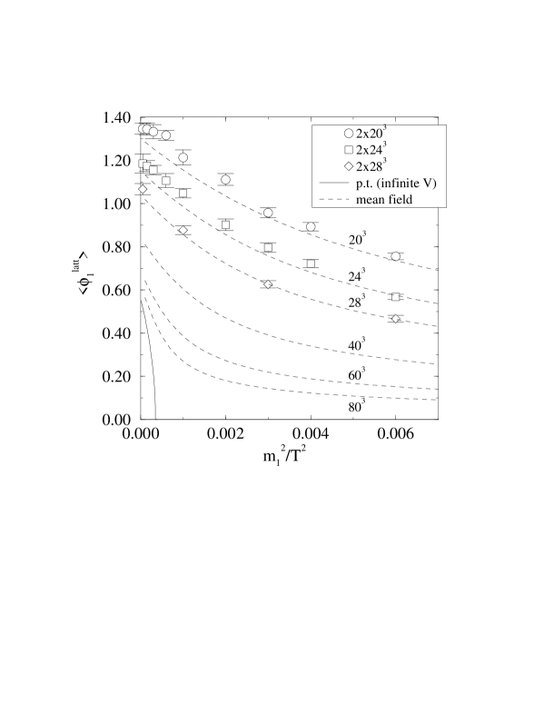
Figure 1: A scan of lattice results, as a function of the continuum parameter $m_{1}^{2}/T^{2}$. The infinite volume perturbative continuum result, as well as finite volume mean field estimates, are also shown. The lattice results are completely compatible with the perturbative ones.

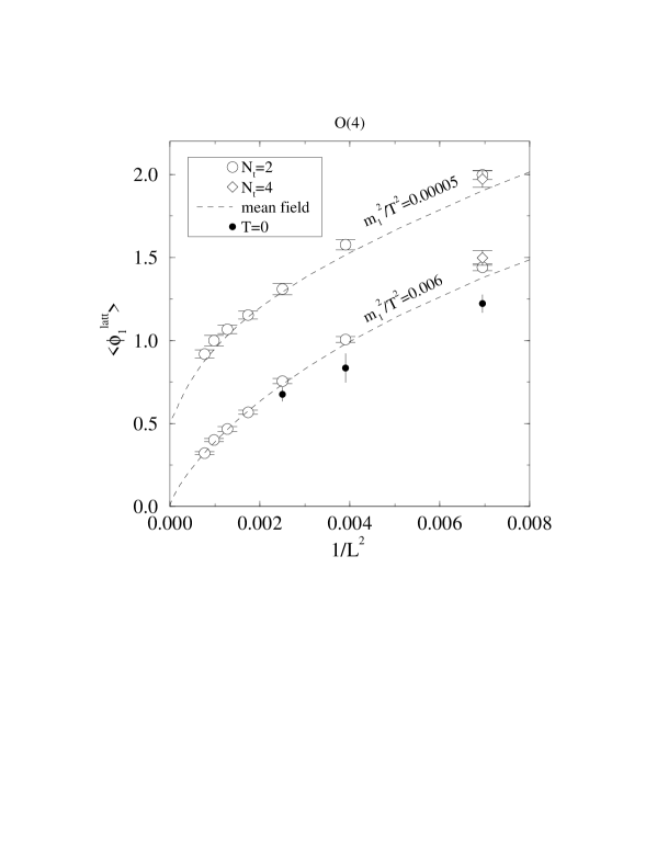
Figure 2: The infinite volume limit for the O(4) field expectation value $\langle\phi_{1}\rangle$ at $m_{1}^{2}/T^{2}=0.00005,0.006$. Mean field estimates are also shown, as well as results from a smaller lattice spacing.

In Fig. 1, we show a scan of continuum parameters, for different volumes. The field is shown in lattice units, $\phi_{1}^{\mbox{\scriptsize latt}}=(a/\sqrt{\kappa_{1}})\phi_{1}^{\mbox{\scriptsize cont}}$. The infinite volume curve computed from the 2-loop effective potential in the theory of eq. (8) is also shown (however, as mentioned, the tree-level result could also be used, as the difference is very small, of order 1%).

It can be seen that the lattice results differ from the continuum perturbative result by quite a significant amount for the volumes used. However, this can be easily understood. Indeed, the finite volume mean field estimates obtained from

$$\langle\phi_{1}\rangle\approx\frac{\int d\hat{\phi}_{1}\hat{\phi}_{1}^{4}\exp[-\frac{1}{T}N^{3}a^{3}V_{\mbox{\scriptsize eff}}(\hat{\phi}_{1})]}{\int d\hat{\phi}_{1}\hat{\phi}_{1}^{3}\exp[-\frac{1}{T}N^{3}a^{3}V_{\mbox{\scriptsize eff}}(\hat{\phi}_{1})]},$$ (22)

where $V_{\mbox{\scriptsize eff}}(\hat{\phi}_{1})$ is the continuum effective potential, $\hat{\phi}_{1}$ denotes the radial component of $\phi_{1}$, and the volume element of an O(4) vector is $d\phi_{1}\propto\hat{\phi}_{1}^{3}d\hat{\phi}_{1}$, are also shown in the figure. They are in perfect agreement with the lattice results.

Next we take two points and look more precisely at the approach to the infinite volume limit. The results are shown in Fig. 2. Again we find perfect compatibility with the perturbative mean field estimates. For the parameter value $m_{1}^{2}/T^{2}=0.00005$, there is inverse symmetry breaking, while for $m_{1}^{2}/T^{2}=0.006$, the symmetry is restored in the infinite volume limit.

The results so far had been obtained with a single lattice spacing, $N_{t}=2$. We have also made simulations with $N_{t}=4$. The results are shown in Fig. 2, after rescaling volumes and units so that they become comparable with those at $N_{t}=2$ (in other words, the volume $4\times 24^{3}$ is represented at the same point as $2\times 12^{3}$, and the field has been normalized so that the data points correspond to the same continuum units). No lattice spacing dependence is seen within the errorbars.

Finally, let us point out that, in principle, the existence of inverse symmetry breaking could also be verified without any reference to perturbative renormalization. In practice, though, this would require huge volumes for the weak couplings we have chosen. However, we have made a few zero temperature runs for the parameters corresponding to $m_{1}^{2}/T^{2}=0.00005$. The results are shown in Fig. 2 with the filled circles. It is seen that the results for $\langle\phi_{1}\rangle$ are indeed smaller than at finite temperature, and certainly consistent with an extrapolation to zero.

In conclusion, we have reiterated what kind of non-perturbative effects there can be in finite temperature phase transitions in scalar theories. The existence of the transition alone can be deduced with perturbation theory, while some of its properties (such as the order) are non-perturbative. With explicit 4d finite temperature lattice simulations, we have verified that the non-perturbative behaviour is indeed in perfect agreement with perturbative estimates, and inverse symmetry breaking takes place.

Appendix

We give here the parameters appearing in the 3d theories in eqs. (3) and (8) with more precision than in the text.

Denoting $c=-0.348725$ and

$$L_{b}(\bar{\mu})=2\ln\frac{\bar{\mu}}{4\pi e^{-\gamma}T}\equiv 2\ln\frac{\bar{\mu}}{\bar{\mu}_{T}},$$ (23)

the $\overline{\mbox{\rm MS}}$ scheme renormalized parameters appearing in eq. (3) are

$$\lambda_{1,3} = T\lambda_{1}(\bar{\mu}_{T})=T\biggl{[}\lambda_{1}(\bar{\mu})-\frac{3}{32\pi^{2}}\biggl{(}\frac{N+8}{9}\lambda_{1}^{2}+\gamma^{2}\biggr{)}L_{b}(\bar{\mu})\biggr{]},$$

$$\lambda_{2,3} = T\lambda_{2}(\bar{\mu}_{T})=T\biggl{[}\lambda_{2}(\bar{\mu})-\frac{3}{32\pi^{2}}\biggl{(}\lambda_{2}^{2}+N\gamma^{2}\biggr{)}L_{b}(\bar{\mu})\biggr{]},$$

$$\gamma_{3} = T\gamma(\bar{\mu}_{T})=T\biggl{[}\gamma(\bar{\mu})-\frac{1}{32\pi^{2}}\biggl{(}4\gamma^{2}+\frac{N+2}{3}\gamma\lambda_{1}+\gamma\lambda_{2}\biggr{)}L_{b}(\bar{\mu})\biggr{]},$$

$$m_{1,3}^{2}(\bar{\mu}) = m_{1}^{2}(\bar{\mu})-\frac{1}{32\pi^{2}}\biggl{(}\frac{N+2}{3}\lambda_{1}m_{1}^{2}+\gamma m_{2}^{2}\biggr{)}L_{b}(\bar{\mu})+\frac{T}{24}\biggl{(}\frac{N+2}{3}\lambda_{1,3}+\gamma_{3}\biggr{)}$$

$$- \frac{1}{32\pi^{2}}\biggl{(}\frac{N+2}{9}\lambda_{1,3}^{2}+\gamma_{3}^{2}\biggr{)}\biggl{(}\ln\frac{3T}{\bar{\mu}}+c\biggr{)},$$

$$m_{2,3}^{2}(\bar{\mu}) = m_{2}^{2}(\bar{\mu})-\frac{1}{32\pi^{2}}\biggl{(}\lambda_{2}m_{2}^{2}+N\gamma m_{1}^{2}\biggr{)}L_{b}(\bar{\mu})+\frac{T}{24}\biggl{(}\lambda_{2,3}+N\gamma_{3}\biggr{)}$$ (24)

$$- \frac{1}{32\pi^{2}}\biggl{(}{\frac{1}{3}}\lambda_{2,3}^{2}+N\gamma_{3}^{2}\biggr{)}\biggl{(}\ln\frac{3T}{\bar{\mu}}+c\biggr{)}.$$

The 3d coupling constants here are scale independent, whereas the mass parameters are not (due to the terms on the latter lines), corresponding to the 2-loop UV-divergences remaining in the super-renormalizable 3d theory. When computing, for instance, the 2-loop effective potential in the 3d theory, this scale dependence gets cancelled. Where not indicated explicitly, the parameters appearing in the expressions in eqs. (24) are renormalized $\overline{\mbox{\rm MS}}$ scheme quantities.

The parameters appearing in the final effective theory in eq. (8) are

$$\bar{\lambda}_{1,3} = \lambda_{1,3}-\frac{3}{16\pi}\frac{\gamma_{3}^{2}}{m_{2,3}},$$ (25)

$$\bar{m}_{1,3}^{2}(\bar{\mu}) = m_{1}^{2}(\bar{\mu}_{T})+\frac{T}{24}\biggl{(}\frac{N+2}{3}\lambda_{1,3}+\gamma_{3}\biggr{)}-\frac{1}{8\pi}\gamma_{3}m_{2,3}$$ (26)

$$+ \frac{1}{32\pi^{2}}\biggl{[}{\frac{1}{4}}\lambda_{2,3}\gamma_{3}-\gamma_{3}^{2}\biggl{(}\ln\frac{3T}{2m_{2,3}}+c+{\frac{1}{2}}\biggr{)}-\frac{N+2}{9}\bar{\lambda}_{1,3}^{2}\biggl{(}\ln\frac{3T}{\bar{\mu}}+c\biggr{)}\biggr{]}.$$

For $\bar{m}_{1,3}^{2}$, the first line is the 1-loop expression and the second line the 2-loop contribution. In these formulas, it is enough to use the 1-loop part of $m_{2,3}^{2}$, given in eq. (5).

References

- [1] S. Weinberg, Phys. Rev. D 9 (1974) 3357.
- [2] G. Dvali and G. Senjanović, Phys. Rev. Lett. 74 (1995) 5178; G. Dvali, A. Melfo and G. Senjanović, Phys. Rev. Lett. 75 (1996) 4559; Phys. Rev. D 54 (1996) 7857; B. Bajc, hep-ph/9805352; G. Senjanović, hep-ph/9805361.
- [3] G. Bimonte, D. Iñiguez, A. Tarancón and C.L. Ullod, Nucl. Phys. B 515 (1998) 345 [hep-lat/9707029].
- [4] G. Bimonte, D. Iñiguez, A. Tarancón and C.L. Ullod, DFTUZ-27-97 [hep-lat/9802022].
- [5] G. Bimonte and G. Lozano, Phys. Lett. B 366 (1996) 248; Nucl. Phys. B 460 (1996) 155; Phys. Lett. B 388 (1996) 692.
- [6] J. Orloff, Phys. Lett. B 403 (1997) 309.
- [7] T.G. Roos, Phys. Rev. D 54 (1996) 2944; G. Amelino-Camelia, Nucl. Phys. B 476 (1996) 255; M. Pietroni, N. Rius and N. Tetradis, Phys. Lett. B 397 (1997) 119.
- [8] P. Ginsparg, Nucl. Phys. B 170 (1980) 388; T. Appelquist and R. Pisarski, Phys. Rev. D 23 (1981) 2305.
- [9] K. Farakos, K. Kajantie, K. Rummukainen and M. Shaposhnikov, Nucl. Phys. B 425 (1994) 67 [hep-ph/9404201]; K. Kajantie, M. Laine, K. Rummukainen and M. Shaposhnikov, Nucl. Phys. B 458 (1996) 90 [hep-ph/9508379].
- [10] A. Jakovác, K. Kajantie and A. Patkós, Phys. Rev. D 49 (1994) 6810; A. Jakovác and A. Patkós, Nucl. Phys. B 494 (1997) 54.
- [11] E. Braaten and A. Nieto, Phys. Rev. D 51 (1995) 6990 and D 53 (1996) 3421; A. Nieto, Int. J. Mod. Phys. A 12 (1997) 1431.
- [12] M.E. Shaposhnikov, in Proceedings of the Summer School on Effective Theories and Fundamental Interactions, Erice, 1996 [CERN-TH/96-280, hep-ph/9610247].
- [13] P. Arnold, Phys. Rev. D 46 (1992) 2628.
- [14] A. Hasenfratz and P. Hasenfratz, Phys. Lett. B 93 (1980) 165; R. Dashen and D.J. Gross, Phys. Rev. D 23 (1981) 2340.
- [15] M. Lüscher and P. Weisz, Nucl. Phys. B 290 (1987) 25.
- [16] Z. Fodor and K. Jansen, Phys. Lett. B 331 (1994) 119; B. Bunk, Nucl. Phys. B (Proc. Suppl.) 42 (1995) 566.