Finite Size Scaling and “perfect” actions:
the three dimensional Ising model.

Abstract

Using Finite-Size Scaling techniques, we numerically show that the first irrelevant operator of the lattice $\lambda\phi^{4}$ theory in three dimensions is (within errors) completely decoupled at $\lambda=1.0$. This interesting result also holds in the Thermodynamical Limit, where the renormalized coupling constant shows an extraordinary reduction of the scaling-corrections when compared with the Ising model. It is argued that Finite-Size Scaling analysis can be a competitive method for finding improved actions.

PACS: 05.50.+q 75.40.Mg 75.40.Cx 11.15.Ha

Keywords: Lattice. Monte Carlo. Perfect actions. Critical exponents. Finite-size scaling.

1 Introduction

The study of the scale-invariance of a system with many-degrees of freedom is of relevance both for the study of phase transitions in Condensed-Matter Physics and for High Energy Physics. The Renormalization Group (RG) is the central concept for these investigations. In both fields it can be turned onto a powerful tool when combined with Monte Carlo (MC) simulations [1]. In this kind of investigations one is only interested in universal properties (in RG language, the leading singularities described by the relevant operators). However, the action used in the simulation is also coupled to irrelevant operators. Their effects can only be neglected in the limit of infinite lattice size and infinite correlation-length. This systematic error is at present the main difficulty to extract meaningful results from the simulation. For phase-transitions studies, the quantitative consideration of the scaling-corrections induced by the irrelevant operators in Finite-Size Scaling (FSS) studies [2] was started in Ref. [3]. At present, the problem is quite well understood, both below [4, 5, 6], and at the upper critical dimension [7].

An action completely decoupled of the irrelevant operators is called a perfect action [8]. From the RG point of view, a perfect action is on the RG-trajectory that leaves the fixed point along the (supposedly unique) relevant direction (the so-called Renormalized Trajectory). It can be easily understood that the effort of finding such an action may be rewarding. In fact, the quest for perfect actions has been very active in the last years (see Ref. [9] and references therein). The perfect action program may be summarized as follows. One first choose a real-space RG transformation, usually keeping a tunable parameter. A finite-dimensional coupling space is chosen, and the RG trajectory is tried to fit in it. The tunable parameter is played with, in order to minimize the truncation errors due to the finite-dimension of the coupling-space [10].

The main difficulty in the perfect action program described above is related with the arbitrariness introduced by the RG transformation and by the coupling-space chosen to parameterize it. Indeed, given a reasonable coupling-space, it is expected to contain a set of points for which scaling-corrections are minimal (this is a working definition of a “perfect” action). It is clear that the most efficient way of locating it cannot be trying different RG group transformations until one of them falls just on it. We will argue that FSS analysis provides a simple and efficient way to locate this privileged set of couplings. To put the argument at work, we have investigated the lattice scalar $\lambda\phi^{4}$ theory in three dimensions. We will show that in this simple two dimensional coupling space it is possible to put the action’s coupling to the first irrelevant operator below the statistical errors. However, the usual lattice gauge-theories simulations are not done in the FSS regime (correlation length $\xi$ much larger than the lattice size $L$), although some interesting calculations have been performed [11]. For this reason, we have also investigated the scaling properties of our “optimal” action in the opposite regime, $L\gg\xi$. We have found again that the effects of the leading irrelevant operator lies below the statistical errors. As a byproduct, we are able to reconcile some discrepancies between MC calculations of the renormalized coupling constant at zero external momentum [12, 13], with a previous field-theoretic estimate [14].

Very recently a similar MC study has been published [15] for the $S=1$ Ising model. The freedom introduced is quite close to ours (we let the spin to be a real number, they only allow it to be $1$,$0$ or $-1$). Thus, it is worthwhile to briefly comment on the differences between the two works. To start with, they use as input the value of a numerically determined universal quantity (basically a Binder cumulant), in order to numerically tune the action. On the contrary, we do not require a previous knowledge of the Binder cumulant. Next, they use their improved action to produce a strong error reduction on the estimates of the Ising critical exponents. We believe this error reduction to be unjustified (see Ref. [6], and section 5).

2 Finite Size Scaling and the best action

To frame the discussion, let us consider a model with only two relevant parameters, the “thermal field”, $t$, and the “magnetic” field, $h$, like for instance the Ising model. The free-energy of a sample of linear size $L$ can be written as [2, 4]

$$f(t,h,\{u_{j}\},L^{-1})=g(t,h,\{u_{j}\})+s^{-d}f_{\mathrm{sing}}(s^{y_{t}}t,s^{y_{h}}h,\{u_{j}s^{y_{j}}\},s/L),\ j\geq 3.$$ (1)

where $s$ is the scale of an (unspecified) RG transformation, and $f_{\mathrm{sing}}$ stands for the singular part, $g$ being analytical. The $y$’s are the eigenvalues of the RG transformation, so that $y_{t},y_{h}>0$, but $0>y_{3}>y_{4}>\ldots$ . A basic assumption of this approach is that the RG-evolution of the couplings is the same as in an infinite system. It is quite common to write $\nu=1/y_{1}$, $\eta=2+d-2y_{h}$ and $\omega=-y_{3}$. From the free-energy, the thermodynamically interesting observables follow by taking derivatives. Let $\xi(L,t)$ be any reasonable definition of the correlation length in a finite lattice (see for instance Ref. [16]). One can obtain a general expression for any observable, $O$ diverging in the thermodynamical limit like $t^{-x_{O}}$:

$$O(L,t)=L^{x_{O}/\nu}\left[F_{O}\left(\frac{\xi(L,t)}{L}\right)+{\mathcal{O}}(L^{-\omega},\xi_{\infty}^{-\omega})\right]\ ,$$ (2)

where $\xi_{\infty}$ is the correlation-length in an infinite lattice. Eq. (2) is most interesting deep in the scaling region ($\xi_{\infty}\gg L$), where the ${\mathcal{O}}(\xi_{\infty}^{-\omega})$ corrections can be safely neglected. It is clear, that in Eq. (2) we have only kept the corrections due to the first irrelevant field, $u_{3}$, (in fact, a full series in $L^{-\omega}$ is to be expected) but similar corrections arise from the others. A radically different correction is produced by the analytical part of the free energy, $g$. When one takes derivatives in Eq. (1) with respect to the “magnetic” field, a not diverging term follows from $g$. This implies that for several important operators like the susceptibility, the Binder cumulant, or the correlation length, a correction like $L^{-\gamma/\nu}$ should be added in Eq. (2), if the multiplicative structure is to be kept.

One can exploit Eq. (2), by comparing the measures taken in two lattices

$$Q_{O}=\frac{\langle O(sL,t)\rangle}{\langle O(L,t)\rangle},$$ (3)

at the value of the “temperature”, for which the correlation length in units of the lattice size is the same in both

$$\left.Q_{O}\right|_{Q_{\xi}=s}=s^{x_{O}/\nu}+A_{Q_{O}}L^{-\omega}+\ldots\ ,$$ (4)

where $A_{Q_{O}}$ is a constant. In this way, not only the critical exponent $x_{O}/\nu$ can be measured, but also information on the scaling corrections $A_{Q_{O}}L^{-\omega}$ can be extracted [5, 6, 17, 18, 19]. Here we encounter an objective property that a perfect action should have: $A_{Q_{O}}$ should be zero for all the observables. Notice that this does not mean that there are no scaling corrections. There is no way to avoid the ${\mathcal{O}}(L^{-\gamma/\nu})\approx{\mathcal{O}}(L^{-2})$ induced by the analytical part of the free energy (they will be there, even if all the irrelevant fields in Eq. (1), $u_{j}$ are set to zero). But we are still not done, because to efficiently locate the points for which $A_{Q_{O}}=0$ something should be known about $x_{O}/\nu$. The most simple procedure is to choose for $O$ a quantity having $x_{O}=0$, like a Binder cumulant, $B$ (see section 3 for its definition).

Therefore, having a simple model, like for instance the Ising model, a simple strategy for improving its scaling behavior is the following. The original model has only a tunable coupling $\beta$, that reaches a critical coupling, $\beta_{\mathrm{c}}$ (in Eq. (1) $t$ can be identified with the “reduced temperature” $(\beta-\beta_{\mathrm{c}})/\beta_{\mathrm{c}}$). We need to extend the action with another coupling, $\lambda$, which can be for instance a next-to-nearest neighbors coupling, a $\lambda\phi^{4}$ term, etc. The critical point $\beta_{\mathrm{c}}$ will extend into a critical line in the ($\beta$,$\lambda$) plane, $\beta_{\mathrm{c}}(\lambda)$. If there is something like a RG fixed point in the ($\beta$,$\lambda$) plane, one should have

$$1=\frac{B(\beta,\lambda,sL)}{B(\beta,\lambda,L)},\ {\mathrm{if}}\ s=\frac{\xi(\beta,\lambda,sL)}{\xi(\beta,\lambda,L)},$$ (5)

which is Eq. (4) in the absence of scaling corrections. We shall show that we can tune $\lambda$ to the condition given in Eq. (5), with moderate numerical effort, and that this yields a quite strong reduction of scaling corrections.

One could object that there is no reason for the Fixed-Point to lie in such a small coupling-space. The answer is twofold. First, there is quite clear empirical evidence that this indeed happens, for instance in the two dimensional Ising model [20], the O(4) Non Linear $\sigma$ Model in three dimensions [5] and in the three dimensional site diluted Ising model, at $80\%$ spin-concentration [18]. Second and most important, we are only demanding that there exists some RG transformation whose Fixed-Point is close (in some sense) to the ($\beta$,$\lambda$) plane, but we are not burdening ourselves with the task of finding it. If it exists, we should be able of finding the fixed-point coordinates with Eq. (5). And that can be done with rather small lattices.

3 The model

We have considered the scalar $\lambda\phi^{4}$ theory in a three dimensional cubic lattice of side $L$, with periodic boundary conditions. The action is given by

$$S=\beta\,\sum_{<i,j>}\phi_{i}\phi_{j}\ +\ \sum_{i}\phi_{i}^{2}\ +\ \lambda\sum_{i}\left(\phi_{i}^{2}\,-\,1\right)^{2}\,,$$ (6)

where the $\phi$’s are real variables. The $\lambda\to\infty$ limit of the model (6) is the Ising model for magnetism. At fixed $\lambda$, for low values of $\beta$ the system is in a $Z_{2}$-symmetric (paramagnetic) phase. There is a critical line, $\beta_{\mathrm{c}}(\lambda)$, separating the paramagnetic phase from the ferromagnetic phase. The full critical line is second order, and it belongs to the Ising Universality Class, excepting the $\lambda=0$ end-point which is the Gaussian model. The MC simulation of (6) is greatly eased by the cluster-methods [21].

The observables to be measured are easily defined in terms of the Fourier transform of the spin-field

$$\widehat{\phi}(\mbox{\boldmath$k$})=\frac{1}{V}\,\sum_{\mbox{\scriptsize\boldmath$x$}}\phi(\mbox{\boldmath$x$})\mathrm{e}^{{\mathrm{i}}\mbox{\scriptsize\boldmath$k$}\cdot\mbox{\scriptsize\boldmath$x$}}\,,$$ (7)

where $V=L^{3}$ is the lattice volume. We have the susceptibilities at zero ($\chi$) and minimal momentum ($F$):

$$\chi=V\,\left\langle|\widehat{\phi}(0)|^{2}\right\rangle\ ,\ F=\frac{V}{3}\,\sum_{\|\mbox{\scriptsize\boldmath$k$}\|=\frac{2\pi}{L}}\left\langle|\widehat{\phi}(\mbox{\boldmath$k$})|^{2}\right\rangle\,,$$ (8)

and the finite-lattice correlation-length [16] and Binder cumulant.

$$\xi=\sqrt{\frac{\chi/F\,-\,1}{4\sin^{2}(\pi/L)}}\ ,\ B=\frac{3}{2}-\frac{\left\langle|\widehat{\phi}(0)|^{4}\right\rangle}{2\left\langle|\widehat{\phi}(0)|^{2}\right\rangle^{2}}\,.$$ (9)

The renormalized coupling constant at zero external momentum can be readily calculated [16]

$$g_{\mathrm{R}}=2\,B(L/\xi)^{D}\ ,\ D=3.$$ (10)

We also measure the nearest-neighbor energy

$$E=\left\langle\sum_{<i,j>}\phi_{i}\phi_{j}\right\rangle,$$ (11)

in order to calculate $\beta$-derivatives and extrapolations [22]. Let us summarize the critical behavior of the different observables:

$${\begin{array}[]{clcccl}x_{\xi}&=&\nu\,,&x_{\chi}&=&\gamma=\nu(2-\eta)\,,\\ x_{g_{\mathrm{R}}}&=&0\,,&x_{\partial_{\beta}\xi}&=&1+\nu\,,\end{array}}$$ (12)

the critical exponents being [6]

$$\nu=0.6294(10)\ ,\ \eta=0.0374(12)\ ,\ \omega=0.87(9).$$ (13)

These MC results are in excellent agreement with the last series estimates [23].

A final remark is that  [12]

$$g_{\mathrm{R}}^{\infty}\equiv\lim_{\beta\to\beta_{\mathrm{c}}^{-}}\lim_{L\to\infty}\,g_{\mathrm{R}}(L,\beta)\neq\lim_{L\to\infty}\lim_{\beta\to\beta_{\mathrm{c}}}\,g_{\mathrm{R}}(L,\beta)\equiv\tilde{g}_{\mathrm{R}}\,,$$ (14)

as Eq. (2) shows.

4 Optimizing $\lambda$

For a first estimate of the Fixed-Point location, we have simulated lattices $L=4,8$ and $16$ in a mesh of $\lambda$ values ($\lambda=0.25,0.5,1.0,1.5$ and $2$). Results in the Ising limit were also available from previous work [6]. We have measured $\left.Q_{B}\right|_{Q_{\xi}=2}$ for lattice-pairs $(4,8)$ and ($8$,$16$), and check for the condition in Eq. (5) . Given the strong statistical correlation between $Q_{\xi}$ and $Q_{B}$, this quotient can be very precisely calculated. One can obtain a $0.2\%$ accuracy in the ($8$,$16$) pair, with nine Pentium Pro hours. The original idea was to use the mesh as starting point for a bisection search of the optimal $\lambda$, but the $\lambda=1$ data fulfilled the condition in Eq. (5) to the achieved accuracy. Moreover, for the lattice pair ($8$,$16$), at $\lambda=1.5$, $Q_{B}$ was at three standard deviations below 1, and at $\lambda=0.5$ was five standard deviations above. From this, one can estimate the optimal $\lambda$ to be $1.0(1)$. The total CPU time was less than two hours of the 32 Pentium Pro machine RTNN.

A more precise location of the optimal $\lambda$ would require not only much more statistics, but also to simulate larger lattices to avoid higher-order scaling corrections (if needed, one could resort to a reweighting method in $\lambda$). Nevertheless our main scope, has been to check if a zero value of $A_{Q_{B}}$ (see Eq. (4)) does imply the vanishing of the ${\mathcal{O}}(L^{-\omega})$ corrections for the other quantities of interest. In other words, if the first irrelevant operator is decoupled. For this, we have simulated at $\lambda=1$, and also at $\lambda=0.5$ and $\lambda=0.25$ for comparison. The total CPU time employed has been about three RTNN months. We remark that such a time-consuming investigation is not an essential part of an action improvement program, but rather a consistency check.

In practice, one is mainly interested in the thermodynamical limit, where the measures are quite less accurate than in the FSS region. For instance one could be interested in measures of exponential tails of propagators, or in measures of renormalized coupling constants. In the model considered in this work maybe the more interesting universal quantity is $g_{\mathrm{R}}^{\infty}$. Even with the high accuracy allowed by the improved cluster estimators [24], we will show that a $10\%$ error in the optimal $\lambda$ is enough to cancel the leading scaling-corrections. In fact the $\xi=2.5$ data are in the continuum limit to our accuracy ($2\%$). In this regime, we have used 6 RTNN days.

5 Numerical Results when $\xi_{\infty}\gg L$

$L$	Ising	$\lambda=1$	$\lambda=0.5$	$\lambda=0.25$
8	0.98146(20)	1.00094(25)	1.01372(30)	1.02949(40)
12	0.98703(23)	1.00075(24)	1.01088(32)	1.02251(35)
16	0.99038(23)	1.00062(26)	1.00817(29)	1.01840(38)
24	0.99324(21)
32	0.99476(28)	0.9997(5)	1.0045(5)	1.0095(7)
48	0.99612(28)
64	0.99702(34)

Table 1: Quotient of the Binder cumulant measured in lattice pairs ($L$,$2L$) where the correlation-lengths in units of the lattice size are the same. Scaling corrections appear as a value different from one.

Figure 1: Universal quantities as a function of $L^{-\omega}$ ($\omega=0.87$), for the four models considered. The lines correspond to quadratic fits, constrained to yield the same infinite-volume extrapolation.

Figure 2: Universal quantities as a function of $L^{-\gamma/\nu}$, for the $\lambda=1$ data. The linear behavior shows that there is no evidence for scaling-corrections others than the analytical ones.

We have simulated in lattices $L=8,12,16,24,32$ and $64$ for $\lambda=1.0,0.5$ and $0.25$. The Elementary Monte Carlo Step (EMCS) was composed of 10 single-cluster flips, followed by a full-lattice Metropolis sweep. We have taken $10^{7}$ measures, separated by four EMCS, excepting $L=64$ where only $2.5\times 10^{6}$ measures were taken. Our values for $\left.Q_{B}\right|_{Q_{\xi}=2}$ are quoted in table 1. From Eq. (4) we can obtain an ($L$ dependent) estimate of $\nu$ and $\eta$, and also of $\left.B(L)\right|_{Q_{\xi}=2}$ and $\left.\frac{\xi}{L}\right|_{Q_{\xi}=2}$. The results are displayed in Fig. 1, where a quadratic fit in $L^{-\omega}$ is presented. The results for the linear term in $L^{-\omega}$ of the $\lambda=1$ data are (fitting independently from the other $\lambda$ values)

$${\begin{array}[]{cccccc}A_{Q_{\partial_{\beta}\xi}}&=&0.004(44)\ ,&\ A_{Q_{\chi}}&=&0.016(25)\,,\\ A_{\xi/L}&=&0.022(23)\ ,&\ A_{B}&=&0.010(21)\,.\end{array}}$$ (15)

Thus, it seems quite clear that for the four quantities shown in Fig. 1, the coefficient of the ${\mathcal{O}}(L^{-\omega})$ corrections changes sign close to $\lambda=1.0$ and that the $\lambda=1.0$ data are compatible with a “perfect” behavior. That would mean that the scaling-corrections may arise from other irrelevant operator, and from the analytical corrections ${\mathcal{O}}(L^{-\gamma/\nu})$. Plotting our data against the analytical corrections, a nice linear behavior is found (see Fig. 2). Therefore, to our precision $\lambda=1$ seems perfectly decoupled from the first irrelevant operator. Operators with $\omega^{\prime}>\omega$ cannot be resolved from the analytical corrections. At this point, one could be tempted of using the fits of Fig. 2 to reduce the error in the infinite volume extrapolation for the critical exponents, as it is done for instance in Ref. [15]. Followed blindly, this criterion reduces the errors in a factor four, or larger when compared to the fit in Fig. 1. But we believe this reduction to be unjustified, because we have tuned $\lambda$ to Eq. (5) numerically, so the condition $A_{Q_{O}}=0$ can only be expected to hold within errors, as shown in Eq. (15). Therefore, the more conservative estimate given in Eq. (13) is to be preferred. If a procedure were designed (numerical or analytical) to largely reduce the errors in $A_{Q_{O}}$, one could expect an improvement of an order of magnitude in critical exponents measures. Nevertheless, we will see below that a truly significant gain will be obtained in the $L\gg\xi$ regime.

A worrying feature of this analysis, is that the scaling corrections for $\eta$ and $\nu$ when $\lambda=0.25$, seem no longer under control. One would say that we need to simulate in significantly larger lattices, to reach the asymptotic regime. We think this to be an effect of the competition with the Gaussian fixed-point at $\lambda=0$. A similar behavior was found in the site diluted Ising model at very small dilution [18].

6 Numerical Results when $\xi\ll L$

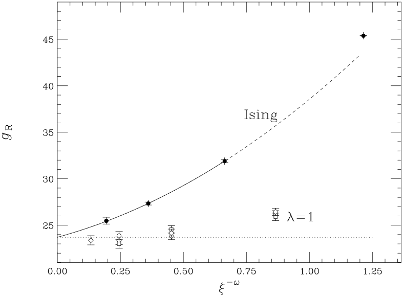
Figure 3: Renormalized coupling constant for $\beta<\beta_{\mathrm{c}}$. The Ising data are taken from Ref. [12] and correspond to $L/\xi=10$. The $\lambda=1$ data are obtained at $L/\xi=6$ (diamonds), $L/\xi=10$ (squares) and $L/\xi=12$ (circles). The horizontal dotted line correspond to the theoretical value.

As an objective test of scaling, we have chosen the renormalized coupling constant. This has been a remarkably difficult quantity to measure until now. Field Theoretic calculations [14] yielded

$$g_{\mathrm{R}}^{\infty}=23.73(2),$$ (16)

which was difficult to reconcile with MC calculations up to correlation-length $\xi=6$ [12]. Moreover, calculations [13] of $\tilde{g}_{\mathrm{R}}$ (see Eqs. (14)) show a worrying decreasing tendency, even suggesting a hyper-scaling violation. Our data in the right-hand side of Fig. 1 quite convincingly show that both the Binder Cumulant and $\xi/L$ are non zero and universal at criticality. Thus, $\tilde{g}_{\mathrm{R}}$ is certainly not zero, as expected. In fact, using the data and procedure of [6], we obtain

$$\tilde{g}_{\mathrm{R}}=5.25(3)$$ (17)

However, the more interesting quantity to calculate is $g^{\infty}_{\mathrm{R}}$ in the reversed limits ordering. The theoretical expectation [25] is that scaling corrections will appear as a power series in $\xi_{\infty}^{-\omega}$.

We have simulated with $\lambda=1.0$, for correlation-lengths $\xi=1.25,2.5,5$ and $\xi=10$, that correspond to $\beta=0.316,0.3588,0.3729$ and $0.3776$, respectively. The EMCS consists of a Swendsen-Wang update of the spin signs, followed by a Metropolis sweep for changing the modulus. Measures were taken every EMCS, using improved estimators [24] (the CPU gain using this estimators is not smaller than a factor of $100$, if the need for $\beta$ reweighting is not as critical as in the FSS region). We have carried out $1.5\times 10^{6}$ EMCS for each lattice size and $\beta$ value. In all cases, but $\xi=10$, we have simulated lattices with $L/\xi\approx 6,10$ and $12$ (we have used lattices $L=8,12,16,24,32,48$ or $64$, depending on $\xi$). The finite-size corrections are expected to drop exponentially with $L$ if periodic boundary conditions are used. At our accuracy level ($2\%$ in the renormalized coupling constant), no significant finite-size corrections are found for $L/\xi\geq 6$ (see Fig. 3). Thus, for $\xi=10$, we have only simulated a $L=64$ lattice.

Our data are plotted together with those for the Ising model of Ref. [12], which have been taken at $L/\xi=10$, thus being quite asymptotic. The horizontal dashed line is the continuum-limit value of Eq. (16). For the Ising model we draw a quadratic fit in $\xi^{-\omega}$ (with $\omega=0.87$), constrained to pass through the value in Eq. (16) (horizontal dotted line), including only data with $\xi>1$. The Ising data at $\xi=0.8$, is somehow far from the quadratic fit, but for $\xi<1$ it is not really surprising that one needs several terms of the $\xi^{-\omega}$ series. In the fit, a significantly non zero coefficient for $\xi^{-\omega}$ is found, as one would expect, and also an important quadratic contribution.

Regarding the $\lambda=1$ data, at $\xi=1.25$, the scaling-corrections are at the $10\%$ level (to be compared with a $50\%$ in the Ising model). From the data we observe a cancellation (within errors) of the linear term and a significant reduction of the quadratic corrections. This could be interpreted as a full cancellation of the $\xi^{-\omega}$ series (full decoupling of the first irrelevant operator). As for $\xi\geq 2.5$ our results are compatible with the Field-Theoretical value, we cannot distinguish if the deviations at $\xi=1.25$ are due to other irrelevant operators or to the analytical corrections (which would be ${\mathcal{O}}(\xi^{-\gamma/\nu})$).

As a final comment, the $\lambda=1.0$ two-point correlator, $\langle\phi(x)\phi(y)\rangle$, does not show a significant improvement on its rotational-invariance when compared with the Ising correlator. That is not really surprising, because we have included only a first-neighbors coupling. So, at correlation-length $\xi\approx 1$ we only have a statistical system with highly anisotropic couplings, which is naturally reflected in the high-momentum behavior of the propagator.

7 Conclusions

We have shown that by eliminating the scaling corrections of the scaling-function of the Binder cumulant in the FSS regime, we obtain a radical improvement of the scaling behavior of other critical quantities, both in the FSS regime and in the thermodynamical limit. This has been done by considering objective properties of the system under study, not depending on an ad hoc RG transformation. This result poses at least three questions. How critical is the choice of the tunable parameter, $\lambda$? (that is, could we have obtained such a good result by considering a next-to-nearest neighbors coupling, for instance?) How can this optimization strategy be implemented in an asymptotically-free theory? (this could be investigated in the two dimensional, $O(3)$ Non-Linear $\sigma$ model, and will be considered in a near future) And last, but not least, will this strategy work in an asymptotically-free lattice-gauge theory?

Regarding the reduction of the errors, the optimal value of $\lambda$ is only approximately known, thus the ${\mathcal{O}}(L^{-\omega})$ corrections cannot be completely disregarded. As a consequence, not true gain in the critical exponents determination is achieved. The situation is quite better in the thermodynamical regime ($L\gg\xi$), where continuum-results (at the $2\%$ level) for the renormalized coupling constant can be obtained at correlation-length $\xi=2.5$. Of course one could object that a judicious use of the FSS method [26] allows to obtain thermodynamical data at very large correlation-length. But also in this case there is a real danger that scaling-corrections will spoil the extrapolation, so a drastic corrections reduction will be of benefit.

References

- [1] I. Montvay and G. Münster, Quantum Fields on a Lattice (Cambridge University Press, 1994); K. Binder and D. W. Heermann, Monte Carlo Simulations in Statistical Physics (Springer-Verlag, 1992).
- [2] M. N. Barber, Finite-size Scaling in Phase Transitions and Critical phenomena, edited by C. Domb and J.L. Lebowitz (Academic Press, New York, 1983) vol 8.
- [3] K. Binder, Z. Phys. B43 (1981) 119.
- [4] H.W.J. Blöte, E. Luijten and J. R. Heringa, J. Phys. A28 (1995) 6289 .
- [5] H. G. Ballesteros, L.A. Fernández, V. Martín-Mayor, and A. Muñoz Sudupe, Phys. Lett. B387 (1996) 125.
- [6] H. G. Ballesteros, L.A. Fernández, V. Martín-Mayor, A. Muñoz Sudupe, G. Parisi and J. J. Ruiz-Lorenzo, cond-mat/9805125.
- [7] H.G. Ballesteros, L.A. Fernández, V. Martín-Mayor, A. Muñoz Sudupe, G. Parisi, J.J. Ruiz-Lorenzo, Nucl. Phys. B512 (1998) 681; J. J. Ruiz-Lorenzo, cond-mat/9804302.
- [8] K. Wilson, in Recent developments of gauge theories, ed. G. ’tHooft et al (Plenum, New York, 1980).
- [9] P. Hasenfratz, F. Niedermayer, Nucl. Phys. B414 (1994) 785; F. Niedermayer, Nucl. Phys. B (Proc. Suppl.) 53 (1997) 56; P. Hasenfratz,G Nucl. Phys. B (Proc. Suppl.) 63 (1998) 53; P. Hasenfratz, hep-lat/9803027.
- [10] L.A. Fernández, A. Muñoz Sudupe, J.J. Ruiz-Lorenzo and A. Tarancón, Phys. Rev. D50 (1994) 5935.
- [11] M. Lüscher, P. Weisz, R. Sommer, U. Wolff, Nucl. Phys. B389 (1993) 247; K. Jansen, C. Liu, M. Lüscher, H. Simma, S. Sint, R. Sommer, P. Weisz, U. Wolff, Phys. Lett. B372 (1996) 275.
- [12] G. A. Baker and N. Kawashima, Phys. Rev. Lett. 75 (1995) 994.
- [13] R. Gupta and P. Tamayo, Int. J. Mod. Phys. C7 (1996) 305; C. Baillie, R. Gupta, K. Hawick and S. Pawley, Phys. Rev. B45 (1992) 10438.
- [14] G. A. Baker, Jr., Quantitative Theory of Critical Phenomena (Academic, Boston, 1990).
- [15] M. Hasenbusch, K. Pinn and S. Vinti, cond-mat/9804186.
- [16] F. Cooper, B. Freedman and D. Preston, Nucl. Phys. B210 (1982) 210.
- [17] H. G. Ballesteros, L.A. Fernández, V. Martín-Mayor, and A. Muñoz Sudupe, Phys. Lett. B378 (1996) 207; Nucl. Phys. B 483 (1997) 707.
- [18] H. G. Ballesteros, L.A. Fernández, V. Martín-Mayor, A. Muñoz Sudupe, G. Parisi and J. J. Ruiz-Lorenzo, cond-mat/9802273 (to be published in Phys. Rev. B).
- [19] H.G. Ballesteros, L.A. Fernández, V. Martín-Mayor, A. Muñoz Sudupe, G. Parisi, J.J. Ruiz-Lorenzo, Phys. Lett. B400 (1997) 346.
- [20] H.G. Ballesteros, L.A. Fernández, V. Martín-Mayor, A. Muñoz Sudupe, G. Parisi, J.J. Ruiz-Lorenzo, J. Phys. A30 (1997) 8379.
- [21] R. H. Swendsen and J. S. Wang, Phys. Rev. Lett. 58 (1987) 86; U. Wolff, Phys. Rev. Lett. 62 (1989) 361; R. C. Brower and P. Tamayo, Phys. Rev. Lett. 62 (1989) 1087.
- [22] M. Falcioni, E. Marinari, M. L. Paciello, G. Parisi and B. Taglienti, Phys. Lett. B108 (1982) 331; A. M. Ferrenberg and R. H. Swendsen, Phys. Rev. Lett. 61 (1988) 2635.
- [23] R. Guida and J. Zinn-Justin, cond-mat/9803240.
- [24] U. Wolff, Phys. Rev. Lett. 60 (1988) 1461.
- [25] F. J. Wegner, Phys. Rev. B5 (1972) 4529.
- [26] M. Lüscher, P. Weisz and U. Wolff, Nucl. Phys. B359 (1991) 221; J. K. Kim, Phys. Rev. Lett. 70 (1993) 1735; S. Caracciolo, R. G. Edwards, A. Pelissetto, A. D. Sokal, Phys. Rev. Lett. 75 (1995) 1895.