Two-dimensional Lattice Gross-Neveu Model
with Wilson Fermion Action
at Finite Temperature and Chemical Potential

Taku Izubuchia)    Junichi Noakia) and Akira Ukawaa,b) Institute of Physicsa), University of Tsukuba
Tsukuba, Ibaraki 305-8571, Japan
Β 
Center for Computational Physicsb)
University of Tsukuba, Tsukuba, Ibaraki 305-8571, Japan
Abstract

We investigate the phase structure of the two-dimensional lattice Gross-Neveu model formulated with the Wilson fermion action to leading order of $1/N$ expansion. Structural change of the parity-broken phase under the influence of finite temperature and chemical potential is studied. The connection between the lattice phase structure and the chiral phase transition of the continuum theory is clarified.

††preprint: UTHEP-383 UTCCP-P-39

I Introduction

In spite of significant effort expended over the years[1], thermodynamic studies of lattice QCD with the Wilson fermion action have been lagging behind those with the Kogut-Susskind action. The origin of difficulty is the explicit breaking of chiral symmetry due to the Wilson term, with ensuing complications in analysis of chiral properties. It has become clear only recently that the finite-temperature phase diagram has an unconventional structure[2], having a region of spontaneously broken parity and flavor symmetry[3, 4, 5, 6] in addition to the usual parity-flavor symmetric phase. While this development has considerably clarified a number of puzzling features observed in numerical simulations in the past[1], there are still questions needing further elucidation. One of the questions is how the continuum limit is to be taken with the new phase diagram. The parity-flavor broken phase has an extension which depends on the temporal lattice size, and the tuning of parameters necessary to achieve a continuum limit having chiral symmetry has not been explored in detail. Another interesting question is how the phase diagram generalizes for finite quark chemical potential corresponding to finite baryon density. As is well known, finite-density studies of lattice QCD have been plagued with serious problems[7]. A conceptual understanding of the phase diagram is a prerequisite in numerical studies of this difficult problem.

In this article we carry out an analytical exploration of these problems in the context of the two-dimensional Gross-Neveu model[8] on the lattice formulated with the Wilson fermion action[9, 10]. The model shares with QCD the feature of asymptotic freedom and spontaneously broken chiral symmetry. Furthermore it is analytically solvable in $1/N$ expansion. These points make the model an useful arena for exploration of theoretical issues with lattice QCD thermodynamics with the Wilson quark action. Indeed the model has provided significant hints for understanding the structure of the finite-temperature phase diagram[2].

In the continuum the phase diagram of the Gross-Neveu model on the plane of temperature $T$ and fermion chemical potential $\mu$ was determined some time ago[11]. In the leading order of $1/N$ expansion, the $(T,\mu)$ plane is divided into two phases, a chirally broken phase at low temperatures and small chemical potential and a symmetric phase at high temperatures and large chemical potential, separated by a phase boundary. Along the phase boundary, the transition is of second order for small chemical potential, which however, changes into a first-order transition for large chemical potential. Our aim in this article will be, first, to determine the phase diagram of the lattice model for finite temporal lattice sizes corresponding to finite temperature and finite chemical potential, and, second, to study how the continuum phase diagram is recovered as one takes the limit of continuum space-time.

This paper is organized as follows. In Sec.Β II, after a brief review of the Gross-Neveu model in the continuum, we formulate the lattice model with the Wilson fermion action at finite temperature and chemical potential, and analyze the behavior of the effective potential toward the continuum limit. In Sec.Β III the phase structure of the model at zero temperature and zero chemical potential is studied. In Sec.Β IV effects of finite temporal lattice size (i.e., of finite temperature) on the phase diagram is examined, and the continuum extrapolation is studied. The case of finite chemical potential is treated in Sec.Β V where we consider in detail how the difference in the order of phase transition observed in the continuum theory arises in the context of the lattice model. We conclude with a summary in Sec.Β VI.

II Analytical Examinations

A Continuum Theory

The Gross-Neveu model in two-dimensional Euclidean continuum space-time is defined by the Lagrangian density,

$\displaystyle{\mathcal{L}}=\bar{\psi}(\gamma_{\mu}\partial_{\mu}+m)\psi-\frac{g^{2}}{2N}[(\bar{\psi}\psi)^{2}+(\bar{\psi}i\gamma_{5}\psi)^{2}],$ (1)

where $\psi$ is an $N$-component spinor field and $g^{2}$ denotes the coupling constant. Our convention for the two-dimensional $\gamma$ matrices is

$\displaystyle\gamma_{1}=\sigma_{2},\ \gamma_{2}=\sigma_{1},\ \gamma_{5}=\sigma_{3}=i\gamma_{1}\gamma_{2}.$ (2)

For massless fermion $m=0$, the model possesses $U(1)$ chiral symmetry defined by

$\displaystyle\psi\to e^{i\theta\gamma_{5}}\psi\ ,\ \bar{\psi}\to e^{-i\theta\gamma_{5}}\bar{\psi}.$ (3)

In terms of the bosonic fields introduced by

$\displaystyle\sigma\equiv-\frac{g^{2}}{N}\bar{\psi}\psi\ ,\ \pi\equiv-\frac{g^{2}}{N}\bar{\psi}i\gamma_{5}\psi\ ,$ (4)

chiral transformation (3) represents a rotation on the $\sigma$-$\pi$ plane by an angle $2\theta$.

Statistical properties of the system at finite temperature $T$ can be examined by restricting the imaginary time extent of the space-time to $\beta=1/T$, and replacing energy integrals for fermions by Matsubara mode sums over half-integer values according to

$\displaystyle k_{2}\to\omega_{n}=\frac{2\pi}{\beta}(n+1/2)\ \ ,\ n\in\bf{Z}.$ (5)

In order to describe the system at finite chemical potential $\mu$, we add ΞΌβ€‹Οˆβ€ β€‹Οˆπœ‡superscriptπœ“β€ πœ“\mu\psi^{\dagger}\psi to ${\mathcal{L}}$ where Οˆβ€ β€‹Οˆsuperscriptπœ“β€ πœ“\psi^{\dagger}\psi is the fermion number operator. These replacements, together with the introduction of the effective fields (4), leads to the action given by

$\displaystyle S=\int_{-\infty}^{+\infty}\frac{dx_{1}}{2\pi}\int_{0}^{\beta}\frac{dx_{2}}{2\pi}\Big{[}\bar{\psi}(\gamma_{\mu}\partial_{\mu}-m-\sigma-i\gamma_{5}\pi+\mu\gamma_{2})\psi-\frac{N}{2g^{2}}(\sigma^{2}+\pi^{2})\Big{]}.$ (6)

To leading order of $1/N$ expansion, the ground state of the model is determined by the minimum of the effective potential $V(\sigma,\pi)$ for a constant $\sigma$ and $\pi$ given by

$\displaystyle V(\sigma,\,\pi)=\frac{1}{2g^{2}}(\sigma^{2}+\pi^{2})-\frac{1}{\beta}\sum_{n=-n_{\rm max}}^{n_{\rm max}-1}\int_{-M}^{+M}\frac{dk}{2\pi}\ln[(\sigma+m)^{2}+\pi^{2}+k^{2}+(\omega_{n}+i\mu)^{2}],$ (7)

where $M$ represents an ultraviolet cutoff and $n_{\rm max}\equiv\beta M/(2\pi)$. In the chiral limit $m\to 0$, $V$ is a function of $s^{2}\equiv\sigma^{2}+\pi^{2}$. At zero temperature and chemical potential, the minimum of the effective potential is located at s=Λ≑2​M​eβˆ’Ο€/g2β‰ 0𝑠Λ2𝑀superscriptπ‘’πœ‹superscript𝑔20s=\Lambda\equiv 2Me^{-\pi/g^{2}}\neq 0, which signals spontaneous breakdown of chiral symmetry. As the cutoff $M$ is removed $M\to\infty$, $g^{2}$ must converge to zero to keep $\Lambda$ finite, that is, the model is asymptotically free.

At finite temperature and chemical potential, Wolff [11] analyzed the effective potential (7) and determined the phase diagram in the $T$-$\mu$ plane, which is reproduced in Fig.Β 1. Inside the boundary ABC chiral symmetry is spontaneously broken, while the region outside of this line is chirally symmetric. The point $B$ is a tricritical point separating a second-order phase boundary AB from a first-order one BC.

B Lattice Theory with Wilson Fermion Action

Consider a two-dimensional lattice of a lattice spacing $a$. The lattice Gross-Neveu model with the Wilson fermion action is defined by[9]

$\displaystyle\mathcal{L}_{\rm lat}$ $\displaystyle=$ $\displaystyle-\frac{1}{2a}\sum_{\mu}[\,\bar{\psi}(x)\,(r-\gamma_{\nu})\,\psi(x+\hat{\mu})+\bar{\psi}(x)\,(r+\gamma_{\mu})\,\psi(x-\hat{\mu})\,]$ (9)
$\displaystyle+\frac{1}{a}(2r+\delta ma)\bar{\psi}(x)\psi(x)-\frac{1}{2N}[\,g_{\sigma}^{2}(\bar{\psi}(x)\psi(x))^{2}+{g_{\pi}^{2}}(\bar{\psi}(x)i\gamma_{5}\psi(x))^{2}\,].$

where $\delta m$ is a mass counterterm. We take the coupling constant $g_{\sigma}^{2}$ and $g_{\pi}^{2}$ for the two four-fermion interaction terms to be different[10], whose reason will become clear below. Hereafter we let Wilson parameter $r$ be unity.

Similar to the continuum theory, we define a pair of bosonic fields according to

$\displaystyle\sigma\equiv-\frac{g_{\sigma}^{2}}{N}\bar{\psi}\psi+\delta m\ ,\ \pi\equiv-\frac{g_{\pi}{}^{2}}{N}\bar{\psi}i\gamma_{5}\psi\ ,$ (10)

In order to consider the system at finite temperature $T$, we take a lattice with $N_{T}=1/(Ta)$ sites in the temporal direction. A finite chemical potential $\mu$ is introduced through a modification of the hopping factor in the temporal direction[12]. The Lagrangian of the model then takes the form,

$\displaystyle\mathcal{L_{\rm lat}}$ $\displaystyle\to$ $\displaystyle-\frac{1}{2a}[\,\bar{\psi}(x)\,(1-\gamma_{1})\,\psi(x+\hat{1})+\bar{\psi}(x)\,(1+\gamma_{1})\,\psi(x-\hat{1})\,]$ (13)
$\displaystyle-\frac{1}{2a}[\,\bar{\psi}(x)\,(1-\gamma_{2})\,e^{-\mu a}\,\psi(x+\hat{2})+\bar{\psi}(x)\,(1+\gamma_{2})\,e\,^{\mu a}\,\psi(x-\hat{2})\,]$
$\displaystyle+\frac{1}{a}(2+\delta ma)\bar{\psi}(x)\psi(x)-\frac{N}{2g_{\sigma}^{2}}(\sigma-\delta m)^{2}-\frac{N}{2g_{\pi}^{2}}\pi^{2}.$

With these modifications, the effective potential $V_{L}=Va^{2}$ in lattice units is given by

$\displaystyle V_{L}(\sigma_{L},\pi_{L})$ $\displaystyle=$ $\displaystyle\frac{1}{2g_{\sigma}^{2}}(\sigma_{L}-\delta m_{L})^{2}+\frac{1}{2g_{\pi}^{2}}\pi_{L}^{2}-\int_{-\pi}^{\pi}\frac{d\xi}{2\pi}\mathcal{J}(\xi)\ ,$ (14)

with

$\displaystyle{\mathcal{J}}(\xi)$ $\displaystyle\equiv$ $\displaystyle\frac{1}{N_{T}}\sum_{n=0}^{N_{T}-1}\ln[A-B\cos(\omega_{n}a+i\mu_{L})],\quad\omega_{n}a\equiv\frac{2\pi}{N_{T}}(n+\frac{1}{2}),$ (15)
$\displaystyle A$ $\displaystyle=$ $\displaystyle 2+(\sigma_{L}+2)^{2}-2(\sigma_{L}+2)\cos\xi+\pi_{L}^{2},$ (16)
$\displaystyle B$ $\displaystyle=$ $\displaystyle 2(\sigma_{L}+2)-2\cos\xi,$ (17)

where $\sigma_{L}\equiv\sigma a,\,\pi_{L}\equiv\pi a,\,\delta m_{L}\equiv\delta ma$ and $\xi=k_{1}a$ are quantities in lattice units.

The Matsubara mode sum in $\mathcal{J}(\xi)$ can be carried out as follows:

$\displaystyle\mathcal{J}(\xi)$ $\displaystyle=$ $\displaystyle\frac{1}{N_{T}}\ln\prod_{n=1}^{N_{T}}\Bigl{[}A-\frac{B}{2}e^{-\mu_{L}-i\pi/N_{T}}e^{2\pi ni/N_{T}}-\frac{B}{2}e^{\mu_{L}+i\pi/N_{T}}e^{-2\pi ni/N_{T}}\Bigl{]}$ (18)
$\displaystyle=$ $\displaystyle\frac{1}{N_{T}}\ln\Bigl{[}\Bigl{(}\frac{B}{2}\Bigl{)}^{N_{T}}e^{EN_{T}}\prod_{n=1}^{N_{T}}(1-e^{-E-\mu_{L}-i\pi/N_{T}}e^{2\pi ni/N_{T}})$ (20)
$\displaystyle\ \ \ \ \ \ \ \ \ \ \ \ \ \ \ \ \ \ \ \ \ \times\prod_{n=1}^{N_{T}}(1-e^{-E+\mu_{L}+i\pi/N_{T}}e^{-2\pi ni/N_{T}})\Bigl{]}$
$\displaystyle=$ $\displaystyle\ln\frac{|B|}{2}+\mu_{L}+\frac{1}{N_{T}}\ln|1+e^{(E-\mu_{L})N_{T}}|+\frac{1}{N_{T}}\ln|1+e^{-(E+\mu_{L})N_{T}}|,$ (21)

where

$\displaystyle E\equiv\left\{\begin{array}[]{ll}\cosh^{-1}(A/B)&\mbox{if}\ A/B>0\\ \cosh^{-1}\bigl{|}A/B\bigl{|}+i\pi&\mbox{if}\ A/B<0\ ,\end{array}\right.$ (24)

and we have used the formula

$\displaystyle\prod_{n=1}^{N}(1+xe^{2\pi ni/N})=1-(-x)^{N}.$ (25)

The real part of $E$ has the meaning of the energy of the fermion one-particle state for a given value of $\sigma_{L}\,,\,\pi_{L}$ and dimensionless space momentum $\xi$.

C Continuum Limit

The lattice Gross-Neveu model as we defined above explicitly breaks chiral symmetry due to the Wilson term. Toward the continuum limit $a\to 0$, an examination of effects of symmetry breaking is possible through an expansion of the effective potential in powers of $a$[10]. We briefly recapitulate the analysis here as it raises an important point for the study of phase diagram in the following sections.

We consider the effective potential (14) at $T=0(N_{T}=\infty)$ and $\mu=0$, and write it as

$\displaystyle V_{L}(\sigma_{L},\,\pi_{L})$ $\displaystyle=$ $\displaystyle\frac{1}{2g_{\sigma}^{2}}(\sigma_{L}-\delta m_{L})^{2}+\frac{1}{2g_{\pi}^{2}}\pi_{L}^{2}-\int_{-\pi}^{+\pi}\frac{d^{2}\xi}{(2\pi)^{2}}\ln\left[D_{0}(\xi)+D_{1}(\xi)\right],$ (26)

where

$\displaystyle D_{0}(\xi)$ $\displaystyle=$ $\displaystyle\sum_{\nu=1,2}\sin^{2}\xi_{\nu}+\left(\sum_{\nu=1,2}(1-\cos\xi_{\nu})\right)^{2}+\sigma_{L}^{2}+\pi_{L}^{2},$ (27)
$\displaystyle D_{1}(\xi)$ $\displaystyle=$ $\displaystyle 2\sigma_{L}\sum_{\nu=1,2}(1-\cos\xi_{\nu}).$ (28)

The continuum limit of the effective potential is determined by terms of ${\cal O}(a^{2})$ with $\sigma_{L}$ and $\pi_{L}$ regarded as ${\cal O}(a)$. Since $D_{1}(\xi)={\cal O}(a)$ while $D_{0}(\xi)={\cal O}(1)$, we make an expansion in terms of $D_{1}(\xi)$ in (26) obtaining

$\displaystyle V_{L}(\sigma_{L},\,\pi_{L})$ $\displaystyle=$ $\displaystyle\frac{1}{2g_{\sigma}^{2}}(\sigma_{L}-\delta m_{L})^{2}+\frac{1}{2g_{\pi}^{2}}\pi_{L}^{2}-\int_{-\pi}^{+\pi}\frac{d^{2}\xi}{(2\pi)^{2}}\ln D_{0}(\xi),$ (29)
$\displaystyle+$ $\displaystyle\sum_{n=1}^{\infty}\frac{(-1)^{n}}{n}\int_{-\pi}^{+\pi}\frac{d^{2}\xi}{(2\pi)^{2}}\frac{D_{1}(\xi)^{n}}{D_{0}(\xi)^{n}}.$ (30)

The integral over $\ln D_{0}(\xi)$ in (30) can be estimated by an expansion around $\sigma_{L}^{2}+\pi_{L}^{2}=0$, paying attention to logarithmic divergence of the first derivative of the integral with respect to $\sigma_{L}^{2}+\pi_{L}^{2}$. The result reads

$\displaystyle\int_{-\pi}^{\pi}\frac{d^{2}\xi}{(2\pi)^{2}}\ln D_{0}(\xi)$ $\displaystyle=$ $\displaystyle C_{0}(\sigma_{L}^{2}+\pi_{L}^{2})-\frac{1}{4\pi}(\sigma_{L}^{2}+\pi_{L}{}^{2})\ln\frac{\sigma_{L}^{2}+\pi_{L}^{2}}{e}+{\mathcal{O}}(a^{4}),$ (31)

where

$\displaystyle C_{0}=0.220634\cdots.$ (32)

In the sum over $n$ in (30) only the terms up to and including $n=2$ contribute to ${\cal O}(a^{2})$, and $\sigma_{L}^{2}+\pi_{L}^{2}$ in $D_{0}(\xi)$ can be set to zero in this limit. We then find that

$\displaystyle\int_{-\pi}^{+\pi}\frac{d^{2}\xi}{(2\pi)^{2}}\frac{D_{1}(\xi)}{D_{0}(\xi)}$ $\displaystyle=$ $\displaystyle 2C_{1}\sigma_{L}+{\cal O}(a^{3}),\qquad C_{1}=\frac{2\sqrt{3}}{9},$ (33)
$\displaystyle\int_{-\pi}^{+\pi}\frac{d^{2}\xi}{(2\pi)^{2}}\frac{D_{1}(\xi)^{2}}{D_{0}(\xi)^{2}}$ $\displaystyle=$ $\displaystyle 4C_{2}\sigma_{L}^{2}+{\cal O}(a^{4}),\qquad C_{2}=\frac{2\sqrt{3}}{27}+\frac{1}{12\pi}.$ (34)

The integrals (33-34) clearly show that the Wilson term distorts the effective potential in the $\sigma$ direction relative to that of $\pi$. Collecting the results together we find

$\displaystyle V_{L}$ $\displaystyle=$ $\displaystyle-\left(\frac{\delta m_{L}}{g_{\sigma}^{2}}+2C_{1}\right)\sigma_{L}+\left(\frac{1}{2g_{\pi}^{2}}-C_{0}\right)\pi_{L}^{2}+\left(\frac{1}{2g_{\sigma}^{2}}-C_{0}+2C_{2}\right)\sigma_{L}^{2}$ (36)
$\displaystyle+\frac{1}{4\pi}(\sigma_{L}^{2}+\pi_{L}^{2})\ln\frac{\sigma_{L}^{2}+\pi_{L}^{2}}{e}+{\mathcal{O}}(a^{3})\ ,$

The necessity for introduction of the two couplings $g_{\sigma}^{2}$ and $g_{\pi}^{2}$ should now be clear[10]: chiral symmetry would not be recovered toward the continuum limit unless one tunes the couplings. The limit of massless fermion further requires a tuning of the mass parameter $\delta m_{L}$ to remove the linear term in $\sigma$. A natural tuning will be

$\displaystyle\frac{1}{g_{\pi}^{2}}=\frac{1}{g_{\sigma}^{2}}+4C_{2}+{\cal O}(a),$ (37)

and

$\displaystyle\frac{\delta m_{L}}{g_{\sigma}^{2}}$ $\displaystyle=$ $\displaystyle-2C_{1}+{\cal O}(a^{2}).$ (38)

Let us introduce the $\Lambda$ parameter through

$\displaystyle\Lambda\equiv\frac{c}{a}e^{-\pi/g_{\sigma}^{2}},\qquad c\equiv e^{2\pi C_{0}-4\pi C_{2}}=0.57160\cdots.$ (39)

With the tuning (37) this corresponds to a coupling renormalization given by

$\displaystyle\frac{1}{2g_{\sigma}^{2}}$ $\displaystyle=$ $\displaystyle C_{0}-2C_{2}+\frac{1}{4\pi}\ln\frac{1}{\Lambda^{2}a^{2}},$ (40)
$\displaystyle\frac{1}{2g_{\pi}^{2}}$ $\displaystyle=$ $\displaystyle C_{0}+\frac{1}{4\pi}\ln\frac{1}{\Lambda^{2}a^{2}},$ (41)

with which the effective potential (in physical units) takes the standard continuum form

$\displaystyle V(\sigma,\,\pi)=\frac{1}{4\pi}(\sigma^{2}+\pi^{2})\ln(\frac{\sigma^{2}+\pi^{2}}{e\Lambda^{2}})+{\mathcal{O}}(a).$ (42)

It is straightforward to extend the above analysis to the case of finite temperature and chemical potential. No new divergences arise in these cases, and the same tuning of parameters $g_{\sigma}^{2},g_{\pi}^{2}$ and $\delta m_{L}$ as specified in (37-38) is necessary for the correct continuum limit. Hereafter, we often use this tuning ignoring the ${\cal O}(a)$ corrections. This is equivalent to taking

$\displaystyle{\bf T}(g_{\sigma}^{2})\equiv\left(-2C_{1}g_{\sigma}^{2}\,,\,(1/g_{\sigma}^{2}+4C_{2})^{-1}\right)$ (43)

as a tuned point on the $(\delta m_{L},g_{\pi}^{2})$ plane.

We learn from the present analysis that understanding of the continuum limit requires an elucidation of the phase diagram of the lattice model in the three-dimensional parameter space of $(g_{\sigma}^{2},g_{\pi}^{2},\delta m_{L})$. This will be our basic viewpoint in the following sections.

III Phase diagram at $T=0$ and $\mu=0$

We start our investigation of the phase structure of the lattice model with the case of zero temperature and zero chemical potential. To leading order in $1/N$ expansion, the ground state of the model is determined by the pair of saddle point equations

$\displaystyle\frac{\partial V_{L}}{\partial\sigma_{L}}$ $\displaystyle=$ $\displaystyle\frac{\sigma_{L}-\delta m_{L}}{g_{\sigma}^{2}}-\left(\sigma_{L}F(\sigma_{L},\pi_{L})+G(\sigma_{L},\pi_{L})\right)=0,$ (44)
$\displaystyle\frac{\partial V_{L}}{\partial\pi_{L}}$ $\displaystyle=$ $\displaystyle\pi_{L}\left(\frac{1}{g_{\pi}^{2}}-F(\sigma_{L},\pi_{L})\right)=0,$ (45)

where

$\displaystyle F(\sigma_{L},\pi_{L})$ $\displaystyle=$ $\displaystyle\int_{-\pi}^{+\pi}\frac{d^{2}\xi}{(2\pi)^{2}}\frac{2}{\sum_{\nu}\sin^{2}\xi_{\nu}+(\sigma_{L}+\sum_{\nu}(1-\cos\xi_{\nu}))^{2}+\pi_{L}^{2}},$ (46)
$\displaystyle G(\sigma_{L},\pi_{L})$ $\displaystyle=$ $\displaystyle\int_{-\pi}^{+\pi}\frac{d^{2}\xi}{(2\pi)^{2}}\frac{2\sum_{\nu}(1-\cos\xi_{\nu})}{\sum_{\nu}\sin^{2}\xi_{\nu}+(\sigma_{L}+\sum_{\nu}(1-\cos\xi_{\nu}))^{2}+\pi_{L}^{2}}.$ (47)

The second equation allows a non-trivial solution with Ο€Lβ‰ 0subscriptπœ‹πΏ0\pi_{L}\neq 0, which corresponds to spontaneous breakdown of parity symmetry, in addition to the parity-symmetric solution $\pi_{L}=0$. If the phase transition between the two phases is continuous, the phase boundary separating them can be determined by examining the limit of the parity-broken solution toward $\pi_{L}\to 0$. This yields the pair of equations

$\displaystyle\frac{\sigma_{L}-\delta m_{L}}{g_{\sigma}^{2}}$ $\displaystyle=$ $\displaystyle\sigma_{L}F(\sigma_{L},0)+G(\sigma_{L},0),$ (48)
$\displaystyle\frac{1}{g_{\pi}^{2}}$ $\displaystyle=$ $\displaystyle F(\sigma_{L},0).$ (49)

The second equation ensures that the pion mass $M_{\pi}$ vanishes along the phase boundary since, for $\pi_{L}=0$, $M_{\pi}$ is given by

$\displaystyle\left(\frac{M_{\pi}}{\Lambda}\right)^{2}=\frac{\partial^{2}V_{L}}{\partial\pi_{L}^{2}}\Biggl{|}_{\pi_{L}=0}=\frac{1}{g_{\pi}^{2}}-F(\sigma_{L},0).$ (50)

The structure of the phase boundary was previously studied for the case of an equal coupling $g_{\sigma}^{2}=g_{\pi}^{2}$ in Refs.Β [3, 2]. We have to extend the analysis treating the couplings as independent.

The pair of equations (48-49) defines a surface in the three-dimensional parameter space $(g_{\sigma}^{2},g_{\pi}^{2},\delta m_{L})$. We shall tentatively call this surface as parity phase boundary. In Fig.Β 2 we show the section of the surface on the $(\delta m_{L},g_{\pi}^{2})$ plane at $g_{\sigma}^{2}=0.8$. The region above the curve corresponds to the parity-breaking solution Ο€Lβ‰ 0subscriptπœ‹πΏ0\pi_{L}\neq 0, while $\pi_{L}=0$ below it. As one moves along the curve from right to left, the value of $\sigma_{L}$ taken as the parameter of the curve decreases from positive to negative values. The bottom of the three valleys of the curve reaches $g_{\pi}^{2}=0$ at $\sigma_{L}=\sigma_{L0}=0,-2,$ and $-4$ from right to left, respectively, where $F(\sigma_{L},0)=+\infty$ and the mass parameter $\delta m_{L}$ equals $\delta m_{L}=\delta m_{L0}(g_{\sigma}^{2})\equiv\sigma_{L0}-g_{\sigma}^{2}G(\sigma_{L0},0)$.

The horizontal line marks the position of equal coupling $g_{\sigma}^{2}=g_{\pi}^{2}$. We observe that there are three parity-broken intervals in between the parity-symmetric ones. Toward the weak-coupling limit $g_{\sigma}^{2}\to 0$, the horizontal line moves toward the bottom of the valley, which in turn converges toward $\delta m_{L0}(0)=\sigma_{L0}=0,-2,-4$. Hence each of the parity-broken intervals narrows to a point at $g_{\sigma}^{2}=0$; the point at $\delta m_{L}=0$ is the conventional continuum limit, while $\delta m_{L}=-2$ ($\delta m_{L}=-4$) represents the point where the doublers with momentum $\xi=(0,\pi)$ and $(\pi,0)$ ($\xi=(\pi,\pi)$) become massless physical modes. These are the results previously obtained in Refs.Β [3, 2].

As we have emphasized in the previous section, however, a proper continuum limit has to be taken along the line specified by (37-38). The point ${\bf T}(g_{\sigma}^{2})$ corresponding to this line without ${\cal O}(a)$ corrections, given in (43), is marked by a cross in Fig.Β 2. The parity-broken interval is significantly narrower near the point, and the location of the point itself is indistinguishable from the curve in the scale of the figure. A more detailed study of the region near the point is clearly needed. As we shall see, the phase structure near the point is far more complex than would seem from Fig.Β 2. An indication is a self-crossing behavior of the curve already visible for the central valley in Fig.Β 2, which also occurs for the right and left valleys.

In Fig.Β 3 we plot an expanded view of the region near the tuned point ${\bf T}(g_{\sigma}^{2})$; we take $g_{\sigma}^{2}=2.0$ for this figure as the structure is enhanced and so easier to draw. The thick curve represents the parity phase boundary, while the set of thin curves are lines of constant $\pi_{L}$, as determined from (44-45), for $0\leq\pi_{L}\leq 0.12$ in steps of 0.02. A number of important features are revealed in this figure. First of all, the boundary curve crosses with itself at the point B (this point differs from the tuned point ${\bf T}(g_{\sigma}^{2})$ marked by a cross, to be discussed below). To understand why the crossing takes place, we note that the right-hand side of (48) behaves as $(\sigma_{L}\ln\sigma_{L}^{2})/2\pi+2C_{1}$ near $\sigma_{L}=0$. Hence (48) regarded as an equation of $\sigma_{L}$ for a given $\delta m_{L}$ has three solutions in the neighborhood of $\delta m_{L}=-2C_{1}g_{\sigma}^{2}$, leading to the self-crossing behavior. Since the existence of three solutions is valid for arbitrarily small values of $g_{\sigma}^{2}$, the crossing persists down to $g_{\sigma}^{2}=0$. Quite clearly there is no guarantee that the boundary curve represents the true phase boundary below the crossing point.

Another important feature is that the lines of constant $\pi_{L}$ spill beyond the boundary curve to the right of the crossing point. In the triangular region DBE formed by the two segments of the boundary curve DB-BE and the envelope ED of lines of constant $\pi_{L}$, the saddle point equations (44-45) have three solutions, one with $\pi_{L}=0$ and two more with Ο€Lβ‰ 0subscriptπœ‹πΏ0\pi_{L}\neq 0. Which of the solutions represent the true minimum can only be determined by examining the value of the effective potential. This is a typical situation where a first-order phase transition occurs.

A detailed numerical investigation of the effective potential shows that the true phase boundary runs as follows. Starting from right, the true phase boundary coincides with the parity phase boundary, and hence being of second order, from the point A to the point D where the envelope of lines of constant $\pi_{L}$ starts out. Beyond this point, the phase transition becomes of first order, and runs along the dashed curve from the point D to the point F which is located on the parity phase boundary curve below the crossing point B. At the point F, the phase transition returns to second order, and runs along the boundary curve from the point F through the crossing point B toward the point C. Altogether the parity-broken phase occupies the region above the line ADFBC.

Below this line the ground state of the model can be examined by the effective potential with $\pi_{L}=0$. The potential no longer depends on $g_{\pi}^{2}$, and as a function of $\sigma_{L}$ has a double well structure. As one varies $\delta m_{L}$ below the point F from right to left, the true minimum switches from a positive to a negative value of $\sigma_{L}$ discontinuously. This leads to a first-order phase transition along the line FH reaching down to $g_{\pi}^{2}=0$. We shall call this line as the $\sigma$ phase boundary. Qualitatively, one may describe the behavior of the system near and below the point F as β€œalmost” exhibiting spontaneous breakdown of chiral symmetry.

We emphasize that the intricate structure involving first-order transitions described above originates from the ${\cal O}(a^{3})$ term of the effective potential $V_{L}$ (i.e., ${\cal O}(a)$ in physical units) which contains terms cubic in $\sigma_{L}$. This contrasts with the leading ${\cal O}(a^{2})$ terms in (36) which gives rise to only simple second-order transitions on the $(\delta m_{L},g_{\pi}^{2})$ plane. Indeed, including the ${\cal O}(a^{3})$ contributions given by

$\displaystyle\delta V_{L}=-\frac{8}{3}C_{3}\sigma_{L}^{3}+2\left[C_{1}^{\prime}-\frac{1}{8\pi}\ln(\sigma_{L}^{2}+\pi^{2}_{L})\right]\sigma_{L}(\sigma_{L}^{2}+\pi^{2}_{L})$ (51)

with

$\displaystyle C_{3}=0.0647\cdots,\qquad C_{1}=0.0904\cdots,$ (52)

to the effective potential (36), one quantitatively reproduces the features of the phase diagram shown in Fig.Β 3.

The phase structure on the $(\delta m_{L},g_{\pi}^{2})$ plane we have discussed for $g_{\sigma}^{2}=2$ remains the same toward $g_{\sigma}^{2}\to 0$ except that the structure as a whole moves down toward $g_{\pi}^{2}=0$ and becomes narrower horizontally. In the weak-coupling limit $g_{\sigma}^{2}=0$, the boundary line degenerates to $1/g_{\pi}^{2}=F(\delta m_{L},0)$ which does not have a self-crossing. The first-order line DF disappears, and the entire phase boundary becomes of second order. We thus find the phase structure in the three-dimensional parameter space $(g_{\sigma}^{2},g_{\pi}^{2},\delta m_{L})$ as schematically drawn in Fig.Β 4.

Let us now discuss the continuum limit, in particular, how the phase structure relates with the tuning of parameters specified by (37-38). The tuned point ${\bf T}(g_{\sigma}^{2})$ without ${\cal O}(a)$ terms (cross in Fig.Β 3) is located slightly to the left and below the point B in the parity-symmetric phase. When one takes the coupling $g_{\sigma}^{2}$ to zero, the relative location of the tuned point and the $\sigma$ phase boundary remains the same. Therefore taking the continuum limit exactly along the tuned point ${\bf T}(g_{\sigma}^{2})$ leads to a negative value of $\sigma$. This, however, does not mean that a continuum limit with a positive value of $\sigma$ is not possible.

As we have already pointed out, the structure around the point F stems from the ${\cal O}(a^{3})$ terms of the effective potential, and hence its size shrinks as a power of $a$. One can estimate the effect of adding (51) to (36) by an order counting. Since $\delta m_{L}$ is the coefficient of the linear term $\sigma_{L}$ in (36), the ${\cal O}(a^{3})$ correction (51) causes a shift of form

$$\delta m_{L}\rightarrow\delta m_{L}+{\cal O}(\sigma_{L}^{2})\sim\delta m_{L}+{\cal O}(a^{2})\,.$$ (53)

Hence the structure has a size of ${\cal O}(a^{2})$ in $\delta m_{L}$. By a similar argument for $g_{\pi}^{2}$, we conclude a size of ${\cal O}(a)$ for $g_{\pi}^{2}$. The point of tuning, on the other hand, has a degree of freedom of ${\cal O}(a^{2})$ for $\delta m_{L}$ and ${\cal O}(a)$ for $g_{\pi}^{2}$ . Therefore one may shift the point of tuning within a rectangular region of size ${\cal O}(a^{2})$ times ${\cal O}(a)$ around the point ${\bf T}(g_{\sigma}^{2})$, including a shift to the right of the point F, in which case the continuum value of $\sigma$ becomes positive.

In order to demonstrate that the correct continuum limit is obtained within the freedom of the choice of the parameters described above, we examine the scaling of two physical observables $\sigma/\Lambda$ and $(M_{\pi}/\Lambda)^{2}$ along the lines given by

$\displaystyle\delta m_{L}$ $\displaystyle=$ $\displaystyle-2C_{1}g_{\sigma}^{2}+\Delta m(a\Lambda)^{2},$ (54)
$\displaystyle{1\over g_{\pi}^{2}}$ $\displaystyle=$ $\displaystyle{1\over g_{\sigma}^{2}}+4C_{2}+\Delta g_{\pi}a\Lambda\,,$ (55)

where $\Delta m$ and $\Delta g_{\pi}$ are ${\cal O}(1)$ constants. We show the solution of the saddle point equation (44) for $\sigma/\Lambda=\sigma_{L}/(a\Lambda)$ for $\Delta m=0,1,2$ and $\Delta g_{\pi}=0$ in Fig.Β 5 as a function of $a\Lambda=c\exp(-\pi/g_{\sigma}^{2})$ where $\Lambda$ is defined in (39). One sees that $\sigma/\Lambda$ converges to the correct continuum result $\sigma/\Lambda=1$ whether the limit is taken on the left ($\Delta m=0$) or the right ($\Delta m=1,2$) of the point F of the phase boundary.

The pion mass $M_{\pi}$ is more interesting since the mechanism[3, 2] which ensures $M_{\pi}=0$ even for finite $a$ no longer works along the segment DF in Fig.Β 3 because of the first-order nature of the phase transition in this part of the phase boundary. We select $\Delta m=1,1.5,2.0$ and tune $\Delta g_{\pi}$ so that the point $(\delta m_{L},g_{\pi}^{2})$ given by (54-55) is placed just under the first-order line DF in the parity-symmetric phase. Solving the saddle point equations (44-45) for $\sigma_{L}$ and substituting the result into (50), we obtain the curve for $(M_{\pi}/\Lambda)^{2}$ plotted in Fig.Β 6 as a function of $a\Lambda$. The squared pion mass vanishes as a power of $a$ toward the continuum limit, demonstrating that the first-order nature of the parity-breaking phase transition along DF does not cause problems.

So far we have concentrated on the phase structure near $\delta m_{L}=0$. The phase structure around $\delta m_{L}=-4$ is obtained by a reflection $\delta m_{L}\to-4-\delta m_{L}$. The phase structure near $\delta m_{L}=-2$ is different. It is symmetric across the $\delta m_{L}=-2$ plane, and the parity phase boundary turned out to be always of second order. In addition a $\sigma$ phase boundary of first-order transition across which the sign of $(\sigma_{L}+2)$ flips exists at $\delta m_{L}=-2$, similar to the line FH in Fig.Β 3.

In the following we concentrate on the phase structure around $\delta m_{L}=0$ relevant for the usual continuum limit.

IV Phase Diagram at Tβ‰ 0𝑇0T\neq 0 and $\mu=0$

Our analysis of the phase diagram for the case of finite temperature and zero chemical potential proceeds in essentially the same way as for the zero-temperature case; choosing a temporal lattice size $N_{T}$ and a value of $g_{\sigma}^{2}$, we analyze the solution of the saddle point equations and the value of the effective potential given by (14-21) with $\mu_{L}=0$ as a function of $g_{\pi}^{2}$ and $\delta m_{L}$.

In Fig.Β 7 we show the result of such an analysis at $g_{\sigma}^{2}=2$ for a set of temporal lattice size $N_{T}$. For large $N_{T}$, the topological structure of the phase boundary remains the same as at $N_{T}=\infty$ corresponding to zero temperature. In particular the left-half of the phase boundary hardly changes. On the other hand, the right-half of the boundary with the first-order segment moves toward upper left. The lower end point of the first-order segment slides up along the second-order part of the boundary for $N_{T}=\infty$. The vertical $\sigma$ phase boundary also moves toward left with the end point.

This structure changes at a threshold value of $N_{T}$, which equals $N_{T}=13$ for $g_{\sigma}^{2}=2$ chosen for Fig.Β 7, when the first-order segment of the boundary disappears. The entire phase boundary becomes a smooth line of second-order transition, along which $\sigma_{L}$ continuously varies from positive to negative values as one traverses the boundary curve from right to left. As may be inferred from this, the vertical $\sigma$ phase boundary also disappears at the threshold temporal lattice size.

To the extent that the first-order $\sigma$ boundary is interpreted as indicative of spontaneous breakdown of chiral symmetry, its disappearance may be regarded as signifying restoration of chiral symmetry. Indeed the value of $\sigma_{L}$ becomes small when the $\sigma$ phase boundary disappears. We illustrate this point in Fig.Β 8 which shows how the effective potential changes from a double-well to a single-well structure across the threshold value of $N_{T}$ at the tuned point ${\bf T}(g_{\sigma}^{2})$ for $g_{\sigma}^{2}=0.8$.

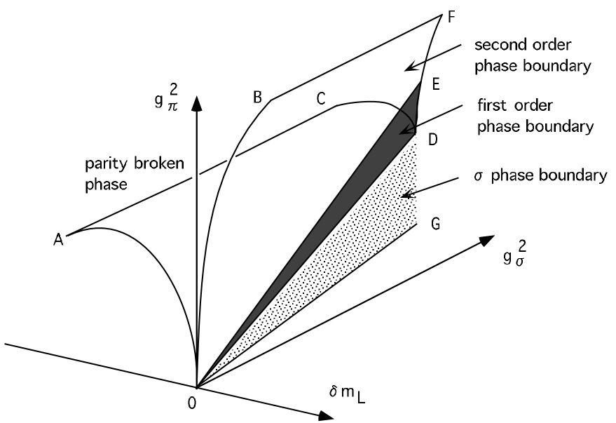
The structural change found as a function of $N_{T}$ for a fixed $g_{\sigma}^{2}$ can be translated into that for a varying $g_{\sigma}^{2}$ with a fixed temporal size $N_{T}$ : as one lowers $g_{\sigma}^{2}$, there is a threshold value $g_{\sigma}^{2}=g_{\sigma c}^{2}(N_{T})$ below which the first-order segment of the parity-broken phase boundary and the vertical first-order $\sigma$ boundary cease to exist. This leads to the three-dimensional phase structure for a fixed and finite $N_{T}$ schematically drawn in Fig.Β 9. Contrary to the $N_{T}=\infty$ case, the boundary curve at $g_{\sigma}^{2}=0$ does not reach the value $g_{\pi}^{2}=0$ since it is given by $1/g_{\pi}^{2}=F(\delta m_{L},0)$ where the function $F(\delta m_{L},0)$ computed for a finite $N_{T}$ is finite and positive at its maximum at $\delta m_{L}=0$.

Let us consider the continuum limit of the model at finite temperature. This limit is defined by simultaneously taking $N_{T}\to\infty$ and $g_{\sigma}^{2}\to 0$ such that

$$\frac{T}{\Lambda}=\frac{\exp(\pi/g_{\sigma}^{2})}{cN_{T}}$$ (56)

is kept fixed. The coupling $g_{\pi}^{2}$ and the mass parameter $\delta m_{L}$ have to be tuned according to (37-38) to restore chiral symmetry. An alternative way to take the limit, which is closer to the method practiced in numerical simulations, is to vary $g_{\sigma}^{2}$ for a fixed $N_{T}$. For each $N_{T}$ this yields physical observables as a function of $T/\Lambda$, and the continuum limit is obtained as a limit of this function as $N_{T}\to\infty$. We follow the latter approach in the following analysis.

A qualitative picture of how finite-temperature transition appears in this approach is as follows. The continuum limit is taken along the line satisfying (37-38), which converges to $(g_{\sigma}^{2},g_{\pi}^{2},\delta m_{L})=(0,0,0)$. Above the threshold value $g_{\sigma}^{2}=g_{\sigma c}^{2}(N_{T})$, this line runs along either side of the lower edge of the parity-broken phase where physical quantities take values similar to those at zero temperature. In particular $\sigma_{L}$ has a non-zero value of positive or negative sign depending on whether the line is on the right or left of the vertical $\sigma$ phase boundary. However, as $g_{\sigma}^{2}$ is lowered below the threshold value, the parity-breaking phase boundary moves up toward larger $g_{\pi}^{2}$, and the $\sigma$ phase boundary disappears. Once the line enters into this region, the value of $\sigma_{L}$ becomes small. In other words, for each fixed temporal size, the threshold value of $g_{\sigma}^{2}$ marks the region of finite-temperature transition.

We illustrate the description above in Fig.Β 10 where we plot $\sigma/\Lambda$ as a function of $T/\Lambda$ calculated along the line ${\bf T}(g_{\sigma}^{2})$ without ${\cal O}(a)$ corrections for several values of $N_{T}$, together with the curve in the continuum limit. We observe that the curves for finite $N_{T}$ smoothly approaches the continuum result drawn by a thick line as $N_{T}$ increases toward $\infty$.

Several remarks are in order with this figure: (i) The negative sign of $\sigma$ is due to the fact, already remarked in Sec.Β III, that the continuum limit is taken on the left side of the $\sigma$ phase boundary. (ii) In the region close to the continuum critical point $T/\Lambda\approx T_{c}/\Lambda=\exp(\gamma_{E}/\pi)=0.56694\cdots$, $\sigma(T)$ has a small discontinuity, as shown in the inset of Fig.Β 10, which reduce with increasing $N_{T}$. This is due to the fact that the tuned point ${\bf T}(g_{\sigma}^{2})$ goes through the vertical $\sigma$ phase boundary as $g_{\sigma}^{2}$ is decreased just before the threshold value is reached (see the relative location of the boundary of $N_{T}=13$ and ${\bf T}(g_{\sigma}^{2})$ in Fig.Β 7). (iii) The value of $\sigma(T)$ after the discontinuity is very small but non-zero for a finite $N_{T}$. It exactly vanishes for $T\geq T_{c}$ only in the limit of $N_{T}\to\infty$.

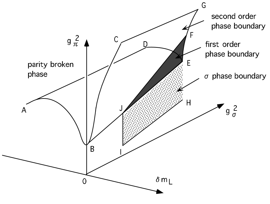
Another possible choice for the continuum limit is to run along the bottom of the valley of the parity-breaking phase boundary for each value of $N_{T}$ (line EJB in Fig.Β 9). The limiting point B of the line at $g_{\sigma}^{2}=0$ has a non-zero value of $g_{\pi}^{2}$. This point, however, reaches the correct continuum limit $(g_{\sigma}^{2},g_{\pi}^{2},\delta m_{L})=(0,0,0)$ as $N_{T}\to\infty$. Above the threshold value of $g_{\sigma}^{2}$ (point J) where the $\sigma$ phase boundary exist, $\sigma(T)$ has two solutions of opposite sign($\sigma^{+}_{L},\sigma^{-}_{L}$). At the bottom of the valley, these two solution are the balancing minima of the effective potential, i.e.,

$$V_{L}(\sigma^{+}_{L})=V_{L}(\sigma^{-}_{L})\,.$$ (57)

At the threshold value of $g_{\sigma}^{2}$, $\sigma^{+}_{L}$ and $\sigma^{-}_{L}$ merge through a second-order singularity corresponding to the second-order phase transition (line JI) marking the end of the first-order $\sigma$ phase boundary.

With this choice of the continuum limit, we obtain the behavior of $\sigma^{+}(T)$ and $\sigma^{-}(T)$ shown by dashed lines in Fig.Β 11 and Fig.Β 12, exhibiting convergence to the continuum result (thick line). A notable property is that the system exhibits a second-order phase transition already for finite values of $N_{T}$ as the line passes through the point J in Fig.Β 9. Also shown in Fig.Β 11 by dotted lines is the difference of the two solutions divided by 2, $(\sigma^{+}_{L}-\sigma^{-}_{L})/2$, which shows a faster convergence to the continuum result.

V Phase Diagram for ΞΌβ‰ 0πœ‡0\mu\neq 0

A The Case of ΞΌβ‰ 0πœ‡0\mu\neq 0 and $T=0$

We now consider the phase diagram for non-zero chemical potential, starting with the case of zero temperature ($N_{T}=\infty$). In this case, from (14-21), the effective potential is given by

$\displaystyle V_{L}=\frac{1}{2g_{\sigma}^{2}}(\sigma_{L}-\delta m_{L})^{2}+\frac{1}{2g_{\pi}^{2}}\pi_{L}^{2}-\int_{-\pi}^{\pi}\!\!\frac{d\xi}{2\pi}\Big{[}\ln(\sigma_{L}+2-\cos\xi)+\max(E,\,\mu_{L})\Big{]}.$ (58)

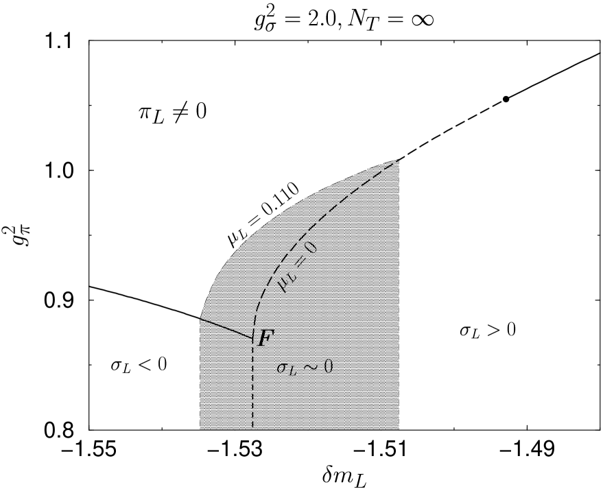
As one expects from this expression, as long as $\mu_{L}$ is small, the phase boundary on the $(\delta m_{L},g_{\pi}^{2})$ plane does not move from that with $\mu_{L}=0$. However, as we show in Fig.Β 13 for $g_{\sigma}^{2}=2$, when $\mu_{L}$ exceeds a threshold value ($\mu_{Lc}\approx 0.09$ for Fig.Β 13), the vertical $\sigma$ phase boundary splits into two vertical first-order boundaries such that $\sigma_{L}$ between the two boundaries is near zero. The end points of the two boundaries slide upwards in the opposite directions along the parity phase boundary for $N_{T}=\infty$, and the phase boundary connecting the two end points, which is of first-order, is convex and moves upward toward larger $g_{\pi}^{2}$. This behavior reflects the fact that the effective potential, which has a double well structure at $\mu_{L}\approx 0$ develops an additional minimum close to $\sigma_{L}=0$ as $\mu_{L}$ increases beyond the threshold value. See Fig.Β 14. Which of the three minima represents the true minimum depends on the value of $\delta m_{L}$, which leads to the double first-order boundaries seen in Fig.Β 13.

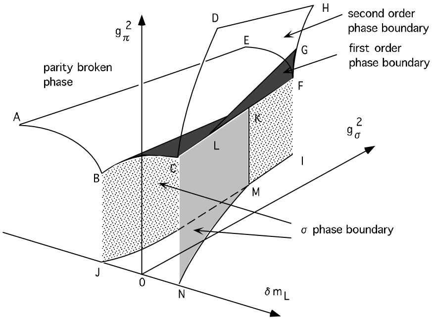
An important point with the behavior described above is that the two vertical first-order boundaries move away from the edge point F of the parity phase boundary at $\mu_{L}=0$. Since the point (37-38) for taking the continuum limit is located near the point F, this means that the system, initially in one of the phases with a non-zero value of $\sigma_{L}$ at $\mu_{L}=0$ undergoes a first-order phase transition when the boundary moves over the point as $\mu_{L}$ increases. After this takes place, the system is in the middle phase with $\sigma_{L}\approx 0$, which qualitatively means that chiral symmetry becomes restored. This, then, is the mechanism by which the lattice model yields the first-order finite density phase transition at zero temperature. These points are illustrated in Fig.Β 15 for $g_{\sigma}^{2}=2.0$. For the tuned point ${\bf T}(g_{\sigma}^{2})$, for example, the left vertical phase boundary moves over the point between $\mu_{L}=0.12$ and 0.13. In Fig.Β 16 we translate the behavior into a schematic three-dimensional phase diagram for $N_{T}=\infty$ and a fixed value of $\mu_{L}$.

B The Case of ΞΌβ‰ 0πœ‡0\mu\neq 0 and Tβ‰ 0𝑇0T\neq 0

Finally we consider the finite-density transition at finite temperature. We examine this case by decreasing the temporal lattice size from $N_{T}=\infty$. The phase structure for $N_{T}=\infty$ found in Sec.Β V A implies that the mechanism of generation of a first-order transition through a splitting of the $\sigma$ phase boundary as $\mu_{L}$ increases will remain operative for large temporal size $N_{T}$. We found this to be the case as shown in Fig.Β 17 for $N_{T}=120$ at $g_{\sigma}^{2}=1.5$.

On the other hand, for small temporal sizes, we expect the behavior to become similar to the finite-temperature and zero chemical potential case examined in Sec.Β III. We plot an example of this case in Fig.Β 18 for which $N_{T}$ is decreased to 28 : the parity-broken phase shrinks, and the first-order segment of the phase boundary and the $\sigma$ phase boundary disappear as one increases $\mu_{L}$. In this case the phase transition is of second order in the continuum limit.

We plot in Fig.Β 19 and Fig.Β 20 curves of $\sigma(T,\mu)/\Lambda$ calculated as a function of $\mu/\Lambda$ for a fixed value of $T/\Lambda$ along the tuned point ${\bf T}(g_{\sigma}^{2})$. A clear discontinuity observed in Fig.Β 19 for $T/\Lambda=0.2$ contrasts sharply with the convergence to second-order behavior seen for $T/\Lambda=0.5$ in Fig.Β 20. This difference reflects the change of order of finite-density transition for large and small temporal lattice sizes discussed above. In the continuum limit we thus find a line of phase transition on the $(\mu,T)$ plane which switches from being of first-order to second order as the critical temperature increases. This agrees with the phase diagram of the continuum theory drawn in Fig.Β 1.

VI Conclusions

In this article we have investigated the phase structure and the continuum extrapolation of the two-dimensional lattice Gross-Neveu model at finite temperature and chemical potential. The choice of the Wilson action for fermions leads to the existence of a parity-broken phase separated from the parity-symmetric phase by a two-dimensional boundary surface in the three-dimensional space of the couplings $(g_{\sigma}^{2},g_{\pi}^{2},\delta m_{L})$ that specifies the model. The phase transition across the surface is generally of second order. However, in the region relevant for the continuum limit, ${\cal O}(a)$ effects of the Wilson term gives rise to a complicated structure, rendering the transition to be of first order in a region whose size vanishes in the continuum limit. The parity-symmetric phase is also divided into subregions by a first-order phase boundary corresponding to different minima of the effective potential. We found that these detailed structures intertwine to lead to the continuum phase diagram reported in Ref.Β [11].

An interesting issue is how much of the detailed structure we found for the Gross-Neveu model has relevance for QCD in four dimensions. Of particular interest is the question that a part of the parity-flavor breaking phase boundary may be of first order. While the necessity of two independent couplings $g_{\sigma}^{2}$ and $g_{\pi}^{2}$ appears to be a specific feature of the Gross-Neveu model, arising from the presence of four-fermion couplings in the model, a distortion of the effective potential for effective meson fields in the $\sigma$ direction by terms odd in $\sigma$ would be present also for QCD, possibly triggering a first-order phase transition.

The relevance of the structure we found for finite chemical potential is more likely; the emergence of three regions corresponding to three different values of $\sigma$ for large $\mu$ is a physical effect, not specifically tied with the use of the Wilson actions for fermions. The crossover from a first-order to second-order transition depending on the critical temperature means, however, that the order of the finite density transition may depend sensitively on the parameters of the model, perhaps the space-time dimension playing an important role[11]. These, then, are the issues which have to be directly addressed in QCD.

Acknowledgments

We thank Y. Taniguchi for informative discussions. One of us (A.Β  U. ) would like to thank F. Karsch for warm hospitality while visiting Zentrum fΓΌr interdisziplinar̈e Forschung (ZiF) of Bielefeld University under the program β€œMulticritical phenomena in complex systems”, where part of the work was carried out. This work is supported in part by the Grants-in-Aid for Scientific Research from the Ministry of Education, Science and Culture (Nos. 2375, 10640246). T.Β I. is supported by Japan Society for the Promotion of Science.

REFERENCES

  • [1] For reviews, see, Y.Β Iwasaki, Nucl.Phys. B (Proc.Suppl.) 42 (1995) 96; A.Β Ukawa, Nucl. Phys. B (Proc.Suppl.) 53 (1997) 106.
  • [2] S.Β Aoki, A.Β Ukawa and T.Β Umemura, Phys. Rev. Lett. 76 (1996) 873; Nucl. Phys. B (Proc. Suppl.) 47 (1996) 511; S.Β Aoki, T.Β Kaneda, A.Β Ukawa and T.Β Umemura, Nucl. Phys. B (Proc. Suppl.)53 (1997) 438.
  • [3] S.Β Aoki, Phys. Rev. D 30 (1984) 2653; 33 (1986) 2377; 34 (1986) 3170; Phys. Rev. Lett. 57 (1986) 3136; Nucl. Phys. B314 (1989) 79.
  • [4] S.Β Aoki and A.Β Gocksch, Phys. Lett. 231B (1989) 449; 243B (1990) 1092; Phys. Rev. D45 (1992) 3845.
  • [5] S.Β Sharpe and R.Β Singleton,Β Jr, hep-lat/9804028.
  • [6] For a different view, see, K.Β Bitar, Nucl. Phys. B (Proc. Suppl.)63 (1998) 829; K.Β Bitar, U.Β Heller, and R.Β Narayanan, Phys. Lett.B418 (1998) 167.
  • [7] For a recent review, see, I.Β M.Β Barbour, S.Β E.Β Morrison, E.Β G.Β Klepfish, J.Β B.Β Kogut and M-P.Β Lombardo, Nucl. Phys. B (Proc. Suppl.)60A (1998).
  • [8] D.Β J.Β Gross and A.Β Neveu, Phys. Rev. D10 (1974) 3235.
  • [9] T.Β Eguchi and R.Β Nakayama, Phys. Lett. 126B (1983) 89.
  • [10] S.Β Aoki and K.Β Higashijima, Prog. Theo. Phys. 76 (1986) 521.
  • [11] U.Β Wolff, Phys. Lett. 157B (1985) 303. For a recent work and references, see also, T.Β Inagaki, T.Β Kouno and T.Β Muta, Int. J. Mod. Phys. A10 (1995) 2241.
  • [12] J.Β B.Β Kogut, H.Β Matsuoka, M.Β Stone, H.W.Β Wyld, S.Β Shenker, J.Β Shigemitsu and D.K.Β Sinclair, Nucl. Phys. B225 [FS], (1983) 93; P.Β Hasenfratz and F.Β Karsch, Phys. Lett. B125 (1983) 308.
Refer to caption
FIG. 1.: Phase diagram of the continuum Gross-Neveu model in the $(\mu/\Lambda,T/\Lambda)$ parameter space. Solid and dashed curves represent a second- and a first-order segment of phase transition restoring chiral symmetry.
Refer to caption
FIG. 2.: Parity phase boundary for $g_{\sigma}^{2}=0.8$ on $(\delta m_{L},g^{2}_{\pi})$ plane. Detailed structure near the tuning point ${\bf T}={\bf T}(g_{\sigma}^{2})$ for taking the continuum limit is shown in Fig.Β 3.
Refer to caption
FIG. 3.: Magnified view of the region near the tuned point ${\bf T}(g_{\sigma}^{2})$ for $g_{\sigma}^{2}=2.0$. Thick curve represents the parity phase boundary while thin lines are contour curves of fixed $\pi_{L}$ values ($\pi_{L}=\,0.02,\,0.04,\,0.06,\,0.08,\,0.10,\,0.12$). True phase boundary consists of AD (second order), DF(first order) and FBC(second order).
Refer to caption
FIG. 4.: Schematic phase diagram for $N_{T}=\infty$ and $\mu_{L}=0$. The phase boundary of the parity-broken phase AOB-CDEF forms a blade whose edge touches the point O $(g^{2}_{\sigma},g^{2}_{\pi},\delta m_{L})=(0,0,0)$. The first order part EOD shrinks to a point at $g_{\sigma}^{2}=0$. Parity-symmetric phase is divided into two phases with $\sigma_{L}<0$ and $\sigma_{L}>0$ by a first-order $\sigma$ phase boundary DOG which vertically drops from the edge OD.
Refer to caption
FIG. 5.: Order parameter $\sigma$ in units of $\Lambda$ as a function of lattice spacing $a\Lambda\equiv c\exp(-\pi/g^{2}_{\sigma})$ calculated for three choices of continuum extrapolation specified by $\Delta m$ for $\Delta g_{\pi}=0$. Sign of $\sigma$ is negative for $\Delta m=0$.
Refer to caption
FIG. 6.: Pion mass squared as a function of lattice spacing $a\Lambda$ under continuum extrapolation. See text for tuning of couplings employed.
Refer to caption
FIG. 7.: Temporal lattice size dependence of phase structure plotted for $N_{T}=\infty$, 16, 14, 13, 12, 10, 8. Phase transition is of first order along dashed lines, while it is of second order along solid lines.
Refer to caption
FIG. 8.: Effective potential for $g_{\sigma}^{2}=0.8$ for temporal lattice size $N_{T}=160$ and $N_{T}=154$. $\delta m_{L}$ is tuned according to ${\bf T}(g_{\sigma}^{2})$.
Refer to caption
FIG. 9.: Schematic phase diagram for fixed and finite $N_{T}$. For small $g^{2}_{\sigma}$, first-order parity-breaking boundary (FJE) and $\sigma$ phase boundary (EJIH) disappear.
Refer to caption
FIG. 10.: Order parameter $\sigma$ as a function of temperature $T$ for $\mu=0$ evaluated for several temporal lattice size along the point ${\bf T}(g_{\sigma}^{2})$ without ${\cal O}(a)$ corrections. Inset shows an expanded view of the critical region.
Refer to caption
FIG. 11.: Positive solution $\sigma^{+}$ as a function of $T$ for $\mu=0$. Couplings are tuned along the edge of the parity-breaking phase boundary (line EJB in Fig.Β 9) for each value of $N_{T}$ . The combination $(\sigma^{+}-\sigma^{-})/2$ is also plotted (see curves specified as β€œ(mid.)”). Inset shows an expanded view of the critical region.
Refer to caption
FIG. 12.: Same as Fig.Β 11 for the negative solution $\sigma^{-}$.
Refer to caption
FIG. 13.: Phase structure for $\mu_{L}=0.110$ and $N_{T}=\infty$ at $g_{\sigma}^{2}=2.0$. Hatched region is the new phase with $\sigma_{L}\approx 0$. Phase transitions between this phase ($\pi_{L}=0,\sigma_{L}\approx 0)$ and other three phases (Ο€Lβ‰ 0,ΟƒL<0,ΟƒL>0formulae-sequencesubscriptπœ‹πΏ0formulae-sequencesubscript𝜎𝐿0subscript𝜎𝐿0\pi_{L}\neq 0,\,\sigma_{L}<0,\,\sigma_{L}>0) are all first order.
Refer to caption
FIG. 14.: Effective potential as a function of $\sigma_{L}$ for $g^{2}_{\sigma}=0.8$ and $N_{T}=\infty$ at the tuned point ${\bf T}(g_{\sigma}^{2})$.
Refer to caption
FIG. 15.: Same as Fig.Β 13 for $\mu_{L}=0,\,0.10,\,0.11,\,0.12,\,0.13$. Symbol T represent the tuned point ${\bf T}(g_{\sigma}^{2})$.
Refer to caption
FIG. 16.: Sketch of phase structure for fixed and finite $\mu_{L}$ for $N_{T}=\infty$. Below a threshold value of $g_{\sigma}^{2}$ the vertical $\sigma$ phase boundary splits into two, both being of first order, enclosing a region with $\sigma_{L}\approx 0$.
Refer to caption
FIG. 17.: Effect of $\mu_{L}$ on the phase structure for large $N_{T}$.
Refer to caption
FIG. 18.: Effect of $\mu_{L}$ on the phase structure for small $N_{T}$.
Refer to caption
FIG. 19.: $-\sigma$ as a function of $\mu$ for $T/\Lambda=0.2$. Couplings are tuned at ${\bf T}(g_{\sigma}^{2})$.
Refer to caption
FIG. 20.: Same as Fig.Β 19 for $T/\Lambda=0.5$.