CERN-TH/98-08

NORDITA-98/30HE

hep-lat/9805013

THE UNIVERSALITY CLASS OF THE ELECTROWEAK THEORY

K. Rummukainen^a, M. Tsypin^b, K. Kajantie^c,d, M. Laine^c,d,
and M. Shaposhnikov^c

^aNordita, Blegdamsvej 17, DK-2100 Copenhagen, Denmark
^bDepartment of Theoretical Physics, Lebedev Physical Institute,
117924 Moscow, Russia
^cTheory Division, CERN, CH-1211 Geneva 23, Switzerland
^dDepartment of Physics, P.O.Box 9, 00014 University of Helsinki, Finland

Abstract

We study the universality class and critical properties of the electroweak theory at finite temperature. Such critical behaviour is found near the endpoint $m_{H}=m_{H,c}$ of the line of first order electroweak phase transitions in a wide class of theories, including the Standard Model (SM) and a part of the parameter space of the Minimal Sypersymmetric Standard Model (MSSM). We find that the location of the endpoint corresponds to the Higgs mass $m_{H,c}=72(2)$ GeV in the SM with $\sin^{2}\theta_{W}=0$, and $m_{H,c}<80$ GeV with $\sin^{2}\theta_{W}=0.23$. As experimentally $m_{H}>88$ GeV, there is no electroweak phase transition in the SM. We compute the corresponding critical indices and provide strong evidence that the phase transitions near the endpoint fall into the three dimensional Ising universality class.

CERN-TH/98-08
NORDITA-98/30HE
May 1998

1 Introduction

The finite temperature phase transition in the Standard Model (SM) is known to be a first order transition for small and a crossover for large Higgs masses [1]. In between there is a critical region at about $m_{H}=$ 75 GeV [2, 3] (see also [4]). The purpose of this paper is to study this critical region in a detailed manner. We shall show that the universality class of the endpoint is that of the three-dimensional (3d) Ising model. We also obtain the value $m_{H,c}<80$ GeV for the endpoint Higgs mass in the SM. Given that the experimental 95% C.L. lower limit is $m_{H}>87.9$ GeV [5], there would be no phase transition, only a crossover, if the physics were that of the SM.

Universality implies a tremendous simplification in the degrees of freedom of the system. Here the first step is the removal of all fermionic and all non-static (not constant in imaginary time) bosonic fields [6]. Equivalently, one integrates out all fields with masses $\mathop{\raise 1.29167pt\hbox{$>$\kern-7.5pt\raise-4.73611pt\hbox{$\sim$}}}\pi T$. This works for equilibrium phenomena in the high $T$ small coupling limit. Furthermore, all masses $\sim gT$ can also be integrated out. Hereby one obtains a 3d effective theory $S[B_{i},A_{i}^{a},\phi_{k}],\,\,i,a=1,2,3,\,\,k=1,\ldots,4$, with SU(2)$\times$U(1) symmetry and a fundamental doublet $\phi$ [7]. The superrenormalizable 3d theory provides a very good approximation to high $T$ 4d physics. The accuracy of the effective description has been discussed in detail in [7]; further corrections to the effective action can also be computed.

The previous steps can be performed perturbatively, but further progress is only possible with numerical lattice Monte Carlo techniques (for reviews, see [8, 9]). In terms of SM physics, these show the existence of a line of first order phase transitions $T_{c}=T_{c}(m_{H})$, $m_{H}<m_{H,c}$, which ends at $T_{c}(m_{H,c})$ and turns into a crossover at $m_{H}>m_{H,c}$. When approaching the endpoint along the first order line, the mass of one of the scalar excitations seems to go to zero suggesting [10] that ultimately all other masses could be integrated out, leaving near $(m_{H,c},T_{c}(m_{H,c}))$ a final effective theory $S_{\mbox{\scriptsize crit}}[\phi^{\prime}]$ containing only one scalar degree of freedom $\phi^{\prime}$.

To be more precise, the electroweak theory with a Higgs doublet contains a massless vector excitation, corresponding to the hypercharge field high in the symmetric phase and to the photon deep in the Higgs phase. The fact that this state is massless at any temperature ensures the “topological” similarity of the phase diagrams of the SU(2)+Higgs and SU(2)$\times$U(1)+Higgs theories [11]. Moreover, the lowest order gauge-invariant coupling of a real scalar to a vector field $\phi^{\prime}F_{ij}F_{ij}$ has a dimensionality greater than 3, and thus the scalar is decoupled from the massless vector in the infrared. Hence, for discussing the universal properties of the theory near the endpoint, we can work with the SU(2)+Higgs theory $S[A_{i}^{a},\phi_{k}]$, disregarding the U(1) interactions. We shall in the following show that the endpoint of this theory belongs to the 3d Ising universality class [12, 13]. The universality class of the 3d O(4) invariant spin model [14, 15], which has also been proposed as a possible candidate [16], can be ruled out.

The matching of the continuum  theories $S[A_{i}^{a},\phi_{k}]\to S_{\mbox{\scriptsize crit}}[\phi^{\prime}]$ is a delicate issue and at this stage we do not determine the couplings of $S_{\mbox{\scriptsize crit}}$, only its universality class. We first discretize the continuum theory at fixed lattice spacing $a$ and determine the critical properties of the discretized theory near the endpoint $(m_{H,c},T_{c}(m_{H,c}))$. This is done by studying the properties of probability distributions of various observables (hopping term, $(\phi^{2}-1)^{2}$, etc) averaged over a finite-volume system (we consider the theory in a cubic box with periodic boundary conditions). We obtain the joint probability distribution of up to 6 observables and analyze it in two ways:

1. We compute the fluctuation matrix, study the dependence of its eigenvalues on the volume and obtain critical indices, which turn out to be consistent with those of the 3d Ising model,

2. We show that for a certain pair of observables, which may be denoted as $M$-like and $E$-like, the joint probability distribution has a very nontrivial form which matches closely the joint distribution of magnetization $M$ and energy $E$ of the 3d Ising model in a box of the same geometry. This guarantees that not only the critical indices, but also higher moments agree with those of the 3d Ising model. As a byproduct we obtain the mapping of the 6-dimensional operator space to the Ising model. This is a fixed lattice spacing version of the critical mapping: $S_{6}[A^{a}_{i},\phi_{k},a]\to S_{\rm Ising}$.

Our method has much in common with, and can be considered as the generalization of, the method used by Alonso et al [17] to locate and study the endpoint of the first order transition line separating the Higgs and confinement phases in the 4d U(1)+Higgs model, and the method developed by Bruce and Wilding [18] for the study of the liquid-gas critical point, both of which rely on considering two-dimensional probability distributions and finding the $M$-like and $E$-like directions. However, our method as well as some aspects of the critical behaviour of our system, differ in many important respects from those in [17, 18].

Finally, an extrapolation to $a\to 0$ will have to be made. There is no change in the universal properties. However, this extrapolation is needed to get the continuum value of the (non-universal) quantity $m_{H,c}$. As mentioned above, this in conjunction with the experimental lower limit implies that the critical region of the 3d effective theory can only be physically relevant in a beyond-the-SM electroweak theory, such as the MSSM.

The plan of the paper is the following. We formulate the problem in Sec. 2 in some more detail, and outline its solution in Sec. 3. In Sec. 4 we review the basic properties of O(N) spin models. Sec. 5 contains a detailed presentation of the method of determining the universality class of the 3d SU(2)+Higgs theory. Asymmetry effects are studied in Sec. 6. In Sec. 7 we summarize the results for the critical properties and for $m_{H,c}$, and we conclude in Sec. 8.

2 Formulation of the problem

At finite temperatures, the static bosonic correlators in the Standard Model and many of its extensions can be derived from the 3d effective action (as discussed above, we omit the U(1) interactions)

$$S = \int\!d^{3}x\biggl{[}\frac{1}{2}{\rm Tr\,}F_{ij}F_{ij}+(D_{i}\phi)^{\dagger}(D_{i}\phi)+m_{3}^{2}\phi^{\dagger}\phi+\lambda_{3}(\phi^{\dagger}\phi)^{2}\biggr{]},$$ (1)

in standard notation. This is a continuum field theory characterized by the dimensionful gauge coupling $g_{3}^{2}$ and by the dimensionless ratios

$$x=\lambda_{3}/g_{3}^{2},\quad y=m_{3}^{2}(g_{3}^{2})/g_{3}^{4},$$ (2)

where $m_{3}^{2}(\mu)$ is the renormalized mass parameter in the $\overline{\mbox{\rm MS}}$ scheme. The relations of $g_{3}^{2},x,y$ to the full theory are computable in perturbation theory, and the relative accuracy thus obtained for non-vanishing one-particle irreducible Green’s functions $G$ that conserve parity, C and CP is [7]

$$\frac{\delta G}{G}\mathop{\raise 1.29167pt\hbox{$<$\kern-7.5pt\raise-4.73611pt\hbox{$\sim$}}}O(g^{3}),$$ (3)

where $\delta G$ is the error in $G$. The fact that there is a suppression of error arises from the ratio of the scales left and integrated out, ${\cal O}(gT/T)$, ${\cal O}(g^{2}T/gT)$, and the third power from the types of higher order operators that have been neglected [7]. Hence, for small coupling, the physics of the 4d theory can be described accurately with a much simpler 3d theory. Explicit derivations have been given in [7, 19].

Instead of using the $\overline{\mbox{\rm MS}}$ scheme, the 3d continuum theory of Eq. (1) can as well be regulated by using a lattice with the lattice constant $a$. The action then is

$$S = \beta_{G}\sum_{\bf x}\sum_{i<j}(1-{\frac{1}{2}}{\rm Tr\,}P_{ij})$$

$$- \beta_{H}\sum_{\bf x}\sum_{i}{\frac{1}{2}}{\rm Tr\,}\Phi^{\dagger}({\bf x})U_{i}({\bf x})\Phi({\bf x}+i)$$

$$+ \sum_{\bf x}{\frac{1}{2}}{\rm Tr\,}\Phi^{\dagger}({\bf x})\Phi({\bf x})+\beta_{R}\sum_{\bf x}\bigl{[}{\frac{1}{2}}{\rm Tr\,}\Phi^{\dagger}({\bf x})\Phi({\bf x})-1\bigr{]}^{2}$$

$$\equiv S_{G}+S_{\mbox{\scriptsize hopping}}+S_{\phi^{2}}+S_{(\phi^{2}-1)^{2}},$$

in standard notation [$\Phi$ is the matrix $\Phi=(i\sigma_{2}\phi^{*},\phi)]$. The two actions in Eqs. (1), (2) give the same physics in the continuum limit $a\rightarrow 0$ if the three dimensionless parameters $\beta_{G},\beta_{H},\beta_{R}$ in Eq. (2) are related to the three dimensionless parameters $g_{3}^{2}a,x,y$ in Eq. (1) by the following equations [20]:

$$\beta_{G} = {4\over g_{3}^{2}a},$$ (5)

$$\beta_{R} = {\beta_{H}^{2}\over\beta_{G}}x,$$ (6)

$$y = {\beta_{G}^{2}\over 8}\biggl{(}{1\over\beta_{H}}-3-{2x\beta_{H}\over\beta_{G}}\biggr{)}+{3\Sigma\beta_{G}\over 32\pi}(1+4x)$$ (7)

$$+{1\over 16\pi^{2}}\biggl{[}\biggl{(}{51\over 16}+9x-12x^{2}\biggr{)}\biggl{(}\ln{3\beta_{G}\over 2}+\zeta\biggr{)}+4.9941+5.2153x\biggr{]},$$

where $\Sigma=3.1759115$ and $\zeta=0.08849(1)$. The two numbers 4.9941 and 5.2153 are specific for the SU(2)+Higgs theory.

The approach to the continuum limit can be accelerated by removing the $O(a)$ errors analytically [21]. For $g_{3}^{2},x$, this can be achieved by reinterpreting the simulation results employing Eqs. (5), (6) as corresponding to

$$\frac{4}{(g_{3}^{2})_{\rm improved}a} = {4\over g_{3}^{2}a}-0.6674,$$ (8)

$$x_{\rm improved} = x-\frac{1}{\beta_{G}}(0.018246+0.195709x+0.583880x^{2}).$$ (9)

For $y$ the issue is more involved, see [21].

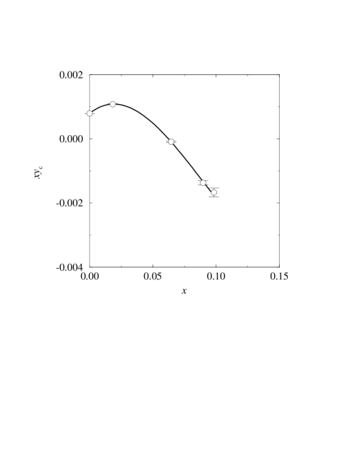
Figure 1: Left: The phase diagram of the 3d SU(2)+Higgs theory. The datapoints are from [10] and from this paper. The value of $x\cdot y_{c}$ at $x\to 0$ is given by the 1-loop effective potential and is hence known analytically. Right: The phase diagram of the 3d scalar $\phi^{4}$ theory in Eq. (10). The value of $x_{I}$ at the endpoint has to our knowledge not been determined. The number 0.002 on the vertical axis is symbolic, as the figure is scale invariant in this direction.

The phase structure of the theory in Eq. (1) is shown in Fig. 1. There is a first order line $y=y_{c}(x)$ for $x<x_{c}$; for $x>x_{c}$ there is only a crossover. The first order line is localised by using the lattice action in Eq. (2) at some finite lattice spacing $a$ and system volume $V$, finding a two-peak distribution in the measurements of any gauge invariant observables and performing the limits $V\to\infty$ and $a\to 0$. At small $x\ll x_{c}$ the two peaks are very asymmetric and well separated, signalling a strong transition. When $x$ approaches $x_{c}$, the two peaks become more symmetric and approach each other. One of the masses, $m_{0^{++}}$ measured by the correlator of $\Phi^{\dagger}\Phi$, becomes smaller than the other masses. One expects that $m_{0^{++}}\to 0$ at $x_{c}$ so that the transition is of the second order there.

In practice, one takes the lattice theory in Eq. (2) at some fixed $\beta_{G}$ and finds the location of the first order line in the plane of the remaining two parameters $(\beta_{H},\beta_{R})$. To approach the continuum limit, one has to repeat the study at higher values of $\beta_{G}$ (we have used $\beta_{G}=5$, 8 and 12).

Since the mass $m_{0^{++}}$ is expected to vanish at the endpoint $x_{c}$, a natural question arising is whether the effective theory in Eq. (1) could be further reduced leaving only the lightest excitations in the final action [22, 23, 10]. Knowing the effective theory would also imply knowledge of the universality class of the second order transition at $x_{c}$. Unfortunately, no systematic perturbative derivation of such an effective action has been found. One problem is that in perturbation theory the vector excitations are massless in the symmetric phase, leading to IR-problems, whereas non-perturbatively they are massive and are to be integrated out. Thus the construction of the effective theory has to be non-perturbative.

As to the functional form of the effective theory, the fact that there is only one light physical scalar degree of freedom, the Higgs particle, naturally leads to the suggestion [1, 10] that the corresponding $\overline{\mbox{\rm MS}}$ continuum effective field theory is

$$S=\int\!d^{3}x\biggl{[}{\frac{1}{2}}\partial_{i}\phi\partial_{i}\phi+h_{I}\phi+{\frac{1}{2}}m_{I}^{2}\phi^{2}+{\frac{1}{4}}\lambda_{I}\phi^{4}\biggr{]}.$$ (10)

We discuss the renormalisation and discretization of this theory in the Appendix. The theory in Eq. (10) is characterized by the scale $\lambda_{I}$ and by the dimensionless ratios $y_{I}=h_{I}/\lambda_{I}^{5/2}$, $x_{I}=m_{I}^{2}(\lambda_{I})/\lambda_{I}^{2}$, where $m_{I}^{2}(\mu)=-6\lambda_{I}^{2}/(16\pi^{2})\log(\Lambda_{m}/\mu)$ is the running mass parameter in the $\overline{\mbox{\rm MS}}$ scheme, and $\Lambda_{m}$ is scale invariant. An otherwise possible cubic term can always be shifted away and this makes $h_{I}$ scale independent. Higher order operators could also exist, but they give contributions suppressed by ${\cal O}(m_{0^{++}}/m_{W})$ where $m_{W}$ stands for all masses, like the inverse vector correlation length, which remain finite at $x_{c}$.

In the critical region the theory in Eq. (10) is in the same universality class as the 3d Ising model in an external magnetic field $h$,

$$Z=\sum_{\{s_{i}\}}\exp[\beta\sum_{\langle ij\rangle}s_{i}s_{j}+h\sum_{i}s_{i}],\qquad s_{i}=\pm 1.$$ (11)

Here $\beta$ is the inverse temperature, the spins $s_{i}$ are located at the sites of a simple cubic lattice, and $\langle ij\rangle$ denotes the pairs of nearest neighbours.

To be more specific about constructing an effective theory such as the one in Eq. (10) (or, for a finite lattice spacing, the one in Eq. (11)), there are two questions to be considered:

1. Which is the functional form (the degrees of freedom; the symmetries; the universality class) of the effective theory?

2. Which is the mapping between the parameters $g_{3}^{2},x,y$ of the original theory, and those of the effective theory (such as $\lambda_{I},x_{I},y_{I}$ of the scalar theory)?

The latter of the two questions is much more difficult than the former one and its solution will not be attempted here. The reason for the difficulty is that the mapping is non-universal and depends on the detailed UV-properties of the original theory. In particular, since the mapping has to be done non-perturbatively on the lattice,

(a) there are finite lattice spacing effects in the lattice formulation in Eq. (2) of the original theory in Eq. (1). These should be identified and removed by an extrapolation to the continuum limit.

(b) there are finite lattice spacing effects in the lattice formulation in Eq. (35) of the effective theory in Eq. (10). These should be controlled in a similar way.

(c) apart from the lattice spacing effects, there are also higher order operators in the effective theory in Eq. (10) applying in the continuum limit, due to the degrees of freedom which have been integrated out. The effects of these are suppressed by $O(m_{0^{++}}/m_{W})$, but they induce errors immediately when one goes away from the critical point (or is at a finite volume).

For the determination of the universality class, in contrast, none of these problems arises. By definition, the universal properties are insensitive to the UV. Hence no extrapolation is needed to overcome (a), and a single finite lattice spacing may be used. However, there is a price to be paid for a finite lattice spacing, which is that there are infinitely many gauge-invariant operators available, and to find the optimal projections on the critical directions, one should take as large an operator basis as possible. No extrapolation to $a\to 0$ is needed for (b), either, and one can directly compare with the known properties of the spin models in the same universality class as the continuum theory considered. Finally, the non-universal errors responsible for (c) vanish at the critical point (but may induce corrections to scaling, etc). In the following we shall mostly concentrate on the universal properties.

3 Outline of the solution of the problem

To study whether the universality properties of the theory in Eq. (1) match those of the scalar theory in Eq. (10), it is sufficient to compare the critical properties of the lattice SU(2)+Higgs theory in Eq. (2) directly with those of the Ising model, Eq. (11).

To gain insight into what is happening at the critical point, it is very helpful to consider two-dimensional probability distributions (joint distributions of two observables) [17, 18]. The motivation is as follows. In the theory in Eq. (2) we have a two-dimensional parameter plane where we find a first order phase transition line which ends in a critical point. In this respect, our system is very similar to such well known systems as the liquid-gas phase transition (where the parameters are the temperature and the pressure) and the Ising model in an external magnetic field (the parameters being the temperature $1/\beta$ and the field $h$).

It has already been checked to considerable precision, both experimentally and by Monte Carlo simulations [18], that in the case of the liquid-gas transition, not only the topology of the critical point is similar to that of the Ising model in an external field, but also the universality class is the same: one can find a linear mapping of a small area around the liquid-gas critical point to the corresponding area around the Ising critical point, such that both systems behave in exactly the same way (up to corrections to scaling at a finite volume).

Our aim is to provide the evidence that the same is also true for our system. Thus we expect to find at the endpoint a temperature-like ($t$-like) direction in the parameter space $(\beta_{H},\beta_{R})$, going tangentially to the phase transition line, and a magnetic field-like ($h$-like) direction, corresponding to the $t$ and $h$ directions of the Ising model.

Our system, as well as the liquid-gas system, lacks the exact symmetry $h\to-h$, which is characteristic of the Ising model. As has been shown for the case of the liquid-gas system, in this case the $h$-like and $t$-like directions are not necessarily orthogonal in the $(\beta_{H},\beta_{R})$ space [24, 18]. Thus, in the vicinity of the critical point of our system, the orthogonal (in the sense $\langle\Delta E\Delta M\rangle=0$) energy-like and magnetization-like observables $E$ and $M$, being derivatives of the free energy over the $t$-like and $h$-like directions in the $(\beta_{H},\beta_{R})$ space, are going to be certain linear combinations of the corresponding terms in the action, that is, of $S_{\mbox{\scriptsize hopping}}$ and $S_{(\phi^{2}-1)^{2}}$, with a possibly non-orthogonal proportionality matrix. In the Ising model the observables $E$ and $M$ just correspond to the first and second terms in Eq. (11).

Before attempting to study the probability distributions of $E$ and $M$, one has to determine the coefficients of these linear combinations. Thus one arrives at the idea of looking at two-dimensional probability distributions: for every configuration generated by Monte Carlo one computes and stores two numbers, $S_{\mbox{\scriptsize hopping}}$ and $S_{(\phi^{2}-1)^{2}}$, thus obtaining their joint probability distribution.

Such distributions are very useful, as they contain a lot of information. Having collected this distribution at some point in the parameter space close to the critical point, one can later find the $E$-like and $M$-like directions; compute the 1-dimensional probability distribution for any linear combination (or even arbitrary function) of $S_{\mbox{\scriptsize hopping}}$ and $S_{(\phi^{2}-1)^{2}}$; refine the estimate for the position of the critical point; and reweight the data to the more precisely determined critical point.

(a)                                                              (b)

(c)

Figure 2: (a) 1000 configurations from the Monte Carlo simulation of the theory in Eq. (2), represented by points in the $S_{(\phi^{2}-1)^{2}}$ vs. $S_{\mbox{\scriptsize hopping}}$ plane, for $x=0.105253,\beta_{G}=8,\beta_{H}=0.349853,V=48^{3}$. (b) 13822 configurations of the same system, for the same parameter values, after a shift and rotation in the coordinate plane. The angle of rotation is chosen to make the elongated distribution in (a) go approximately horizontally. (c) 20000 configurations of the 3d Ising model on a $58^{3}$ lattice at the critical point $\beta_{c}=0.221654,\ h=0$, on “minus the energy” ($0<\sum_{\langle ij\rangle}\delta_{s_{i}s_{j}}<3\cdot 58^{3}$) vs. magnetization ($-58^{3}<\sum_{i}s_{i}<58^{3}$) plane.

To give a concrete view of what is happening, Fig. 2(a) shows the distribution of 1000 configurations obtained near the endpoint, plotted on the $S_{(\phi^{2}-1)^{2}}$ (vertical axis) vs. $S_{\mbox{\scriptsize hopping}}$ (horizontal axis) plane. One can see that the distribution appears to be extremely elongated, and the points tend to concentrate on its sides. The density in the middle is somewhat smaller, thus a two-peak distribution is produced by projecting on either of the axes. Rotating the coordinate system in such a way that the new $x$-axis goes along our distribution, while the new $y$-axis is orthogonal to it, and changing scales, we obtain the distribution plotted in Fig. 2(b). This should be compared with Fig. 2(c) which shows 20000 configurations of the 3d Ising model at the critical point on “minus the energy” (vertical axis: $\sum_{\langle ij\rangle}\delta_{s_{i}s_{j}}$) vs. magnetization (horizontal axis: $\sum_{i}s_{i}$) plane. The qualitative similarity with Fig. 2(b) is striking. At the same time, there are small discrepancies: the distribution in Fig. 2(b) is slightly asymmetric, and considerably thicker than the one in Fig. 2(c). Comparing with Fig. 2(c), one observes that the new $x$- and $y$-axes correspond, with reasonable precision, to $M$-like and $E$-like directions. Note that a projection onto the $M$-like direction produces a two-peak probability distribution, while the $E$-like projection is single-peaked.

The task now is to put the similarity between SU(2)+Higgs and Ising models on a quantitative basis, and to demonstrate that the discrepancies disappear when $V\to\infty$. Note, however, that already the distribution in Fig. 2(b) suggests that O(4) universality is excluded; O(4) would not produce 2-peak distributions like those in Fig. 2(c) and thus cannot match the data in Fig. 2(b) [see Fig. 3(c)].

At this point it is interesting to compare our two-dimensional distributions, depicted in Fig. 2, with those obtained in [17] near the endpoint of the first order phase transition line separating the Higgs and confinement phases in the 4d U(1)+Higgs theory. First, the distributions in [17] demonstrate almost independent fluctuations of $M$ and $E$, while in our case the “boomerang” shape implies that their fluctuations are obviously not independent. Secondly, the distributions in [17] do not show any visible asymmetry, while we see a clear residual asymmetry that can be attributed to corrections to scaling. These differences are probably due to the fact that while the critical point of the 4d model corresponds to a trivial effective theory (this is corroborated by the critical indices obtained in [17], which are compatible with the mean field values), in our case the effective theory, being 3-dimensional, is governed by a nontrivial fixed point.

4 Spin models

Let us start by reviewing some basic properties of simple spin models. The Ising model is defined by Eq. (11). For O(N) models, on the other hand, the spins $s_{i}$ of the Ising model are replaced by $N$-dimensional unit vectors ${\bf s}_{i}$, and the partition function becomes

$$Z=\int\{d{\bf s}_{i}\}\exp[\beta\sum_{\langle ij\rangle}{\bf s}_{i}\cdot{\bf s}_{j}+{\bf h}\cdot\sum_{i}{\bf s}_{i}].$$ (12)

Let us call the first term in the exponent the energy variable $E$, and the next term the magnetic variable $M$:

$$E=-\sum_{\langle ij\rangle}{\bf s}_{i}\cdot{\bf s}_{j},\quad M=\frac{\bf{h}}{|\bf{h}|}\cdot\sum_{i}{\bf s}_{i}.$$ (13)

The characteristics of the model at the critical couplings $\beta=\beta_{c}$, $|{\bf h}|=|{\bf h}_{c}|=0$ are contained in probability distributions in the $(M,E)$-plane, as a function of the volume of the system. When the variances of the distributions are normalized to unity, the distributions have a universal form in the large volume limit; the results for the Ising, O(2) and O(4) models are shown in Fig. 3. To reduce statistical noise, these contour plots, as well as the contour plots in the following pictures, have been smoothed by $3\times 3$ matrix averaging. That is, before plotting, the occupation number in every bin is replaced by the average over 9 bins forming a square around it. The bin size has been chosen sufficiently small so that smoothing does not induce any significant broadening of the peaks.

     

(a)                                                              (b)

(c)

Figure 3: The smoothed and normalized probability distributions, at the critical point, for (a) the Ising model at the volume $58^{3}$, (b) the O(2) spin model at $64^{3}$, (c) the O(4) spin model at $64^{3}$. The $x$-axis is the magnetic direction and the $y$-axis the energy direction.

To quantify the characteristics of the probability distributions, one can compute different moments. Let $\Delta E\equiv E-\langle E\rangle$, $\Delta M\equiv M-\langle M\rangle$. Then the moments of interest are:

1. Second moments (specific heat, magnetic susceptibility):

$$\chi_{E} = \langle(\Delta E)^{2}\rangle/L^{3},$$ (14)

$$\chi_{M} = \langle(\Delta M)^{2}\rangle/L^{3},$$ (15)

where $L^{3}$ is the volume of the system. The behaviour of these moments as a function of $L$ is characterized by critical exponents:

$$\chi_{E}\propto L^{\alpha/\nu},\quad\chi_{M}\propto L^{\gamma/\nu}.$$ (16)

The known results for the exponents appearing here are [25, 14, 26, 27, 28]:

model $\gamma$ $\alpha$ $\nu$ $\gamma/\nu$ $\alpha/\nu$ Ising 1.24 0.11 0.63 1.96 0.17 O(2) 1.32 -0.01 0.67 1.96 -0.015 O(4) 1.47 -0.25 0.75 1.96 -0.33

The exponent $\nu$ is the correlation length critical exponent.

2. Higher moments. These characterize for instance the symmetry features of the probability distributions. In particular, all spin models have, for $n=1,2,\ldots$,

$$\langle(\Delta M)^{2n+1}\rangle=0.$$ (17)

As examples of non-zero values, let us mention that for the 3d Ising model in a large cubic box with periodic boundary conditions, the value of the following ratio is known with high precision [29]:

$$\frac{\langle(\Delta M)^{4}\rangle}{\langle(\Delta M)^{2}\rangle^{2}}=1.604(1).$$ (18)

The asymmetry of the energy distribution of the same system is characterized by

$$\frac{\langle(\Delta E)^{3}\rangle}{\langle(\Delta E)^{2}\rangle^{3/2}}\approx-0.36\\$$ (19)

(this value corresponds to the simple cubic Ising model on a $58^{3}$ lattice, where deviations from scaling due, in particular, to the presence of a large regular part in the energy, are still non-negligible).

These ratios, as well as the critical exponents, are universal quantities which can be used to quantify the similarity or dissimilarity of the endpoint of the SU(2)+Higgs theory with different spin models.

5 Detailed study of the critical region

As discussed above, our computational strategy is based on collecting joint probability distributions of several observables (initially two, as in Fig. 2, and then up to six, as discussed below) for the system in Eq. (2) in a cubic box with periodic boundary conditions. These are used to

1. find the position of the critical point,

2. determine the $M$-like and $E$-like directions in the space of observables,

3. perform finite size scaling (FSS) to compute critical indices, by studying how the fluctuations of $M$-like and $E$-like observables at the critical point depend on the system size,

4. determine higher moments, such as the skewness of $E$.

Our analysis is based on simulations at $\beta_{G}=5$ with the lattice sizes and statistics shown in Table 1. In each case the measurements are separated by 4 overrelaxation sweeps and one heat bath/Metropolis sweep. The update algorithms used are described in Ref. [10]. The relatively coarse lattice spacing was chosen in order to allow for larger physical volumes, and thus reduce the corrections to scaling at any given lattice size.

lattice measurements $16^{3}$ 200000 $24^{3}$ 200000 $32^{3}$ 300000 $40^{3}$ 350000 $48^{3}$ 400000 $64^{3}$ 400000

Table 1: The set of simulations for $\beta_{G}=5$. All simulations have been performed at $x=0.112706$, $\beta_{H}=0.362835$, and later reweighted to the estimated position of the infinite volume critical point: $x=0.11331593$, $\beta_{H}=0.36288657$.

5.1 Locating the critical point

Let us first recall how one locates the critical point in the case of a one-dimensional, rather than a two-dimensional, parameter space, such as in the case of the spin models in Eq. (12). Here the critical point is known to occur at $h=0$, and the only parameter which remains to be found is $\beta_{c}$.

In this case the procedure commonly used is the “intersection of Binder cumulants” [30]. It is based on the following general idea. Consider the system in a finite box of given geometry (say, cubic) with given boundary conditions (say, periodic). Consider any observable (for example, magnetization), averaged over the system. Make a Boltzmann ensemble of configurations, for each configuration measure this observable and thus construct its probability distribution. Then, if the system is exactly at the critical point and scaling is valid, the form of this probability distribution should be independent of the system size; only its scale will be changing. Thus any characteristics such as those in Eqs. (18), (19), designed to be sensitive to the form of probability distribution but not to the rescaling of the observable, will behave in the following typical way: when plotted as a function of a parameter (for spin systems, as a function of $\beta$) for several lattice sizes, all plots intersect at the value of the parameter that corresponds to the critical point. This provides a convenient way to locate it.

This approach can easily be generalized to the case of a two-dimensional parameter space. The main idea remains the same: the critical point is a point where the form of two-dimensional distributions, such as those in Fig. 2, does not depend on the system size, up to a possibly nonorthogonal linear transformation. To locate the critical point, one now needs two characteristics. For example, if one has somehow found the $M$-like direction, one can consider $\langle(\Delta M)^{4}\rangle/\langle(\Delta M)^{2}\rangle^{2}$ and $\langle(\Delta M)^{3}\rangle/\langle(\Delta M)^{2}\rangle^{3/2}$. The former is sensitive to a deviation from the critical point along the (continuation of) the first order transition line, while the latter is sensitive to a deviation across the line. Finding the intersection of these cumulants for two lattice sizes now implies solving a system of two equations for two variables.

The procedure just described is completely general (however, it remains to be understood how to find the $M$-like direction; see Sec. 5.2) and does not depend on any conjecture about the universality class of the critical point. However, it appeared not to be very practical, the main stumbling block being its sensitivity to corrections to scaling, which are in our case non-negligible, as demonstrated by Fig. 2.

A modification of this approach which is more stable against deviations from scaling, relies on a conjecture about the universality class of the critical point. Indeed, if we expect the critical point to belong to the 3d Ising universality class, we know that in the scaling limit $\langle(\Delta M)^{4}\rangle/\langle(\Delta M)^{2}\rangle^{2}=1.604(1)$ [29], $\langle(\Delta M)^{3}\rangle/\langle(\Delta M)^{2}\rangle^{3/2}=0$. By solving these equations, one can find the apparent location of the critical point for each lattice size separately. The consistency of the conjecture about the universality class can be checked later: the lattice size dependence of the position of the apparent critical point should follow the known correction to scaling behaviour.

As a variant, one can use the whole probability distribution $P(M)$, which is known quite precisely for the 3d Ising model, rather than its moments, and require that the apparent critical point for the given lattice size be a point where $P(M)$ matches most favourably the Ising $P(M)$, say, by the $\chi^{2}$ criterion. This method has been used in [18] for locating the liquid-gas critical point.

The method we chose to use in practice is as follows. Assume that we have determined an $M$-like direction, as explained in the next Section. To compute the position of the apparent critical point for a given lattice size we have reweighted the data for the corresponding lattice (Table 1) to a trial value of $(x,\beta_{H})$ which translates to $(\beta_{H},\beta_{R})$ according to Eq. (6), computed the probability distribution of the $M$-like observable $P(M)$ and tuned $(x,\beta_{H})$ so that

1. the two peaks of $P(M)$ are of equal weight,

2. the ratio of the peak value of $P(M)$ (the average height of the two peaks) to $P(M)$ at the minimum between the peaks equals the corresponding ratio for the 3d Ising model at the critical point [31]:

$$P_{\mbox{\scriptsize max}}/P_{\mbox{\scriptsize min}}=2.173(4).$$ (20)

The criterion based on the ratio $P_{\mbox{\scriptsize max}}/P_{\mbox{\scriptsize min}}$ appeared to be less sensitive to asymmetric corrections, which are most pronounced at the tails of $P(M)$, than the usual one based on the fourth order cumulant in Eq. (18).

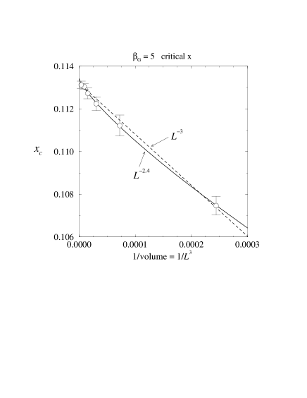
Figure 4: The reweighted $x_{c}$ from simulations at $\beta_{G}=5,x=0.112706$, as a function of the volume.

The resulting dependence of the apparent position of the critical point on the lattice size is shown in Fig. 4. It follows nicely the law based on Ising-type corrections to scaling, the deviation of $x_{c}$ from the limiting value behaving as

$$x_{c}(L)-x_{c}(\infty)\propto L^{-(\Delta+1)/\nu}\approx L^{-2.4},$$ (21)

where $\Delta=0.52(4)$ is the universal correction to scaling exponent for the 3d Ising universality class. Thus the determination of the critical point based on the expected Ising-like properties is completely consistent. However, the statistical errors of the datapoints are large enough so that a regular $L^{-3}$ -behaviour cannot be ruled out, either. Nevertheless, the variation of the infinite volume critical point is quite small, and it has a negligible effect on the analysis below. The infinite volume result, determined by the $L^{-2.4}$-fit, is $x_{c}(\infty)=0.1133(25)$. In the following analysis we always reweight the data to the critical point $x_{c}=0.11331593,\,\beta_{H}=0.36288657$. Due to the strong correlations in coupling constants both have to be fixed to a high numerical precision.

5.2 Determining M-like and E-like observables

We observed that even the problem of locating the critical point, to say nothing of further quantitative analysis, depends on finding the $M$-like direction in the space of observables. In Fig. 2, this is done by letting the $M$-like direction go along the probability distribution, and taking the $E$-like to be orthogonal to it. The result appears to be very encouraging, by the eye, when compared with the 3d Ising distribution in Fig. 2(c). This approach relies on the fact that the distribution is extremely elongated, and becomes even more so with growing lattice size, fluctuations of $M$ growing much faster than those of $E$: $\langle(\Delta M)^{2}\rangle/\langle(\Delta E)^{2}\rangle\propto L^{(\gamma-\alpha)/\nu}\approx L^{1.8}$.

The determination of the $M$-like and $E$-like directions can now be put on a quantitative basis as follows. Take the probability distribution $P(S_{\mbox{\scriptsize hopping}},S_{(\phi^{2}-1)^{2}})$. Compute the fluctuation matrix and find its eigenvectors. The larger eigenvalue will give $\langle(\Delta M)^{2}\rangle$, the smaller one $\langle(\Delta E)^{2}\rangle$, while the corresponding eigenvectors will give the $M$-like and $E$-like directions.

The procedure just described is identical to the one used in [17] and completely ignores the possibility that the $M$-like and $E$-like directions can be nonorthogonal in the original basis chosen [24, 18]. However we have found that both this simplistic procedure and its generalization to a larger space of observables, which is discussed below, work extremely well for our system, while the more sophisticated approach of [18] runs into serious difficulties. This seems to be an interesting point that deserves some discussion, as it probably means that asymmetric corrections to scaling play a more prominent role in our system than in the liquid-gas models (see also Sec. 6).

The method of [18] employs the matching of the probability distribution of a linear combination of the two basic observables to $P(M)$ known from the 3d Ising model at criticality, to find the $M$-like direction simultaneously with the apparent critical point (performing a search in 3-dimensional space: two parameters for a trial critical point, plus one parameter for a trial $M$-like direction). After that, the $E$-like direction is found by matching the distribution of a trial linear combination of observables to the 3d Ising $P(E)$.

One of the key statements of [18] is that the pronounced asymmetry of two-peak probability distributions of various observables at the critical point can be attributed to the fact that they are actually mixtures of $M$ and $E$, while the distribution of $M$ itself comes out completely symmetric, within the accuracy of the simulation. One can, however, raise the following question: is it not possible that the perfect symmetry of $P(M)$ emerges as an artefact of the procedure (optimization of its matching to the exactly symmetric $P(M)_{\mbox{\scriptsize Ising}}$)?

(a)

(b)

(c)

Figure 5: The probability distributions $P(M,E)$ (left) and $P(M)$ (right) at the infinite volume critical point, for the volumes (a) $16^{3}$, (b) $32^{3}$, (c) $64^{3}$. It is seen how the distribution becomes more symmetric for increasing volumes. The $M$ and $E$ directions have been found with a 6-dimensional fluctuation matrix analysis, see Sec. 5.2.1.

This problem can be also put as follows. We have the two-dimensional probability distribution for our system, as in Fig. 2(b), now as a function of four parameters: the trial critical point and two trial directions for $M$ and $E$ (not necessarily orthogonal). On the other hand, we have the corresponding $P(M,E)_{\mbox{\scriptsize Ising}}$ for the Ising model at criticality, Fig. 2(c), with its projections $P(M)_{\mbox{\scriptsize Ising}}$ and $P(E)_{\mbox{\scriptsize Ising}}$. The question is, is it a good idea to look for the $M$-like and $E$-like directions by requiring that just the one-dimensional projections of Figs. 2(b) and 2(c) onto the horizontal and vertical axes match each other? Should not one rather match the whole distributions?

Obviously, in the absence of deviations from scaling it would make little difference whether to match the whole distributions or their one-dimensional projections: both methods would converge to the same result, corresponding to a perfect matching. The problem, however, becomes nontrivial when there are deviations from scaling, especially the asymmetric ones. Concretely, we have found that for our system, an application of the procedure in [18] appeared to be completely misleading.

Figure 6: This figure shows that it is possible to find a direction for $M$ that provides a perfectly symmetric $P(M)$, but only at the price of reducing the symmetry of $P(M,E)$. The data are the same as in Fig. 5(a).

The observation is that for practically achievable lattices, there is a significant asymmetry in two-dimensional distributions, as seen in Fig. 2(b). This asymmetry appears to be unremovable (more precisely, only a relatively small part of it can be removed) by any choice of (nonorthogonal) directions for $M$ and $E$. This can be understood when one notices that one of the characteristic features of this asymmetry is the difference of areas under the two peaks of the probability distribution (see also Figs. 5), which cannot be cured by any linear transformation, even nonorthogonal, as such a transformation keeps the ratio of areas invariant.

Thus if we try to symmetrize the two-dimensional distribution (or match it to the Ising form Fig. 2(c)), a considerable asymmetry remains and, notably, $P(M)$ comes out considerably asymmetric (Fig. 5, right). At the same time, matching $P(M)$ to $P(M)_{\mbox{\scriptsize Ising}}$ easily finds the “$M$-like” direction that ensures a perfect matching and thus symmetric $P(M)$ (Fig. 6). But this optimization of the symmetry of the one-dimensional projection is achieved at the price of greatly reducing, rather than improving, the symmetry of the two-dimensional histogram as a whole and thus should be considered completely misleading!

Thus we have found the following important differences between our system and the liquid-vapour models [18]:

1. Our system demonstrates non-negligible asymmetric corrections to scaling. These show up in two-dimensional distributions and cannot be removed by any choice of $M$ and $E$. As a consequence, asymmetries of various one-dimensional distributions are mostly caused by them, and not so much by the admixture of $E$, as in [18].

2. In our system, we do not find much evidence of the possible nonorthogonality of the $M$-like and $E$-like directions. Deviations from orthogonality, if any, can be safely neglected, in clear distinction from [18] where they played quite a prominent role.

     

Figure 7: The dependence of the probability distribution $P(M,E)$ on the number of observables, for a $\beta_{G}=5$, $64^{3}$ lattice. Left: The diagonalized fluctuation matrix for two observables $S_{\mbox{\scriptsize hopping}}$, $S_{(\phi^{2}-1)^{2}}$, see Eq. (2). Right: The same for four observables, $S_{G}$, $S_{\mbox{\scriptsize hopping}}$, $S_{\phi^{2}}$, $S_{(\phi^{2}-1)^{2}}$. It is seen that the distribution becomes sharper, or thinner, as the basis is expanded. Using six observables leads to a still sharper distribution, see Fig. 5(c).

In conclusion, after having tried four methods for determining the $M$-like and $E$-like directions,

(a) finding the eigenvectors of the fluctuation matrix [17],

(b) matching $P(M)$ to $P(M)_{\mbox{\scriptsize Ising}}$, $P(E)$ to $P(E)_{\mbox{\scriptsize Ising}}$ [18],

(c) matching $P(M,E)$ to $P(M,E)_{\mbox{\scriptsize Ising}}$,

(d) maximizing the symmetry of $P(M,E)$,

we arrived at the conclusion that the method (a) works best for our system, method (b) appears to be misleading, and methods (c) and (d) produce results consistent with (a), while being much more difficult to implement and use. One of the tricky points is the multidimensional minimization of the difference of two Monte Carlo generated two-dimensional probability distributions, which is typically a very noisy function (the problem is alleviated by first smoothing the histograms, then minimizing their difference). Another stumbling block of the method (c) is that a seemingly harmless manifestation of deviations from scaling — the excessive thickness of $P(M,E)$ compared with $P(M,E)_{\mbox{\scriptsize Ising}}$ — has a very strong effect on their difference, in terms of $\chi^{2}$, making it impossible to achieve a good matching.

5.2.1 Extending the space of observables

The main observation so far was that while the form of the probability distribution at the critical point comes out strikingly similar to that of the 3d Ising model, as demonstrated by Figs. 2(b,c), there are still differences (asymmetry and thickness) that are decreasing with growing lattice size, but relatively slowly, so that, for example, the elimination of the thickness would require prohibitively large lattice sizes.

The situation can be considerably improved by further generalizing the procedure of determining the $M$-like and $E$-like observables. The reasoning behind this is as follows. If we consider any arbitrary observable (say, $S_{\mbox{\scriptsize hopping}}$), it behaves at the critical point more or less like magnetization, and its probability distribution also looks very similar to the distribution of magnetization, the main feature being the double-peak structure. However, it shows a certain asymmetry, which eventually goes down to zero with growing lattice size. This can be understood as a consequence of the fact that we expect any observable to behave at the critical point as a sum of $M$-like, $E$-like and regular contributions. Their dependence on the lattice size is different and is governed, correspondingly, by $L^{\gamma/\nu}$, $L^{\alpha/\nu}$ and $L^{0}$. On large lattices the magnetic contribution is always dominating, so any given observable starts behaving as the $M$-like.

From this point of view, when we study the joint distribution of two observables and find the $M$-like and $E$-like directions as the primary axes of the corresponding very elongated fluctuation ellipse, we are actually finding the $E$-like direction as a linear combination of observables in which the dominating $M$-like terms cancel each other. Thus the consideration of two-dimensional distributions provides a way to disentangle the dominant ($M$-like) and subdominant terms. However, it becomes clear that within this approach the $E$-like observable will collect all subdominant terms, both actually $E$-like and regular.

Thus one arrives at the idea that a further separation of $E$-like and regular contributions could be achieved by generalizing the procedure to more observables than two. The hope is to “purify” the $E$ (for $M$ there is little difference, as it outweighs everything else by orders of magnitude anyway).

Figure 8: The joint probability distribution of observables corresponding to the largest (horizontal axis) and second largest (vertical axis) eigenvalues of the $4\times 4$ fluctuation matrix of the terms in Eq. (2).

To begin with, we have considered the 4-dimensional space of observables, these observables being the four terms in the action in Eq. (2). Diagonalizing the $4\times 4$ matrix $\langle(S_{i}-\langle S_{i}\rangle)(S_{j}-\langle S_{j}\rangle)\rangle$ for the $64^{3}$ lattice $(\beta_{G}=5)$ resulted in the eigenvalues and -vectors shown in Table 2. We observe a pronounced hierarchy of eigenvalues, similar to the previously considered case of two observables, Fig. 2(a). The largest eigenvalue corresponds, as expected, to $M$. However, $E$ turns out to correspond, somewhat surprisingly, to the smallest eigenvalue, rather than to the second largest one, while the two eigenvalues in the middle correspond to regular directions. This is substantiated both by analysing the dependence of the eigenvalues on the lattice size and by looking at the joint probability distributions of various pairs of the 4 observables corresponding to the 4 eigenvectors. The joint distribution of projections onto eigenvectors corresponding to the largest and to the smallest eigenvalue is depicted in Fig. 7(right); projections onto eigenvectors corresponding to the largest and to the second largest eigenvalue produce a strikingly different pattern, Fig. 8, signalling that the second largest eigenvalue does indeed correspond to a regular observable: its fluctuations are Gaussian-like and independent from those of $M$.

It is evident in Fig. 7 that the extension of the space of observables from two- to four-dimensional does indeed considerably reduce the deviation of $P(M,E)$ from the 3d Ising scaling form. The most notable effect is the reduction of the excessive thickness of $P(M,E)$. Now the question is, what happens if we further extend the space of observables, having in mind that if one wants to sort out $E$ as well as possible, one would like it to correspond to an eigenvalue which is not the smallest one (as the smallest one is just collecting all unresolved contributions). Thus we have added two additional observables: the sum of the absolute values of the Higgs field, and the analog of the hopping term, where the Higgs matrices have been replaced by SU(2) matrices, dividing out the length of the Higgs field:

$$\tilde{S}_{R}\equiv\sum_{\bf x}R({\bf x}),\quad\tilde{S}_{L}\equiv\sum_{{\bf x},i}{\frac{1}{2}}{\rm Tr\,}V^{\dagger}({\bf x})U_{i}({\bf x})V({\bf x}+i),$$ (22)

where $\Phi({\bf x})=R({\bf x})V({\bf x})$, $R\geq 0,\,V\in$ SU(2).

Now the energy eigenvalue appears to be the fourth of six, in descending order, and we observe further significant reduction of difference between $P(M,E)$ and $P(M,E)_{\mbox{\scriptsize Ising}}$, as seen in Fig. 5(c).

One could continue extending the space of observables (in principle, there are infinitely many gauge invariant operators to be considered), but these six operators seem to be enough for our purposes.

The coefficients of the different eigenvectors in terms of the original operators in Eqs. (2),(22), together with the eigenvalues, are shown in Table 2. We observe the following:

1. While the eigenvectors corresponding to the three largest eigenvalues are relatively stable with respect to an increase in the number of basis vectors, the $E$ direction changes considerably. However, the final critical distributions, critical indices, etc, are quite stable.

2. The largest eigenvalue, the magnetic one, is about 4 orders of magnitude larger than the next largest, for the volumes used.

3. The second largest eigenvalue consists almost solely of the plaquette term of the action, and conversely, the plaquette term contributes significantly only to the second eigenvalue. Thus, the plaquette term is practically decoupled from the other modes.

4. At very large volumes the energy eigenvalue will overtake the two regular eigenvalues above it and become the second largest one (Sec. 5.3). However, for the range of volumes studied here, the hierarchy shown in Table 2 was preserved.

direction	$\lambda$	$c_{1}$	$c_{2}$	$c_{3}$	$c_{4}$	$c_{5}$	$c_{6}$
4 operators
$M$	1.28$\times 10^{10}$	0.05142	0.72590	-0.68564	-0.01808	–	–
regular	8.51$\times 10^{5}$	0.9965	0.008	0.083	0.0049	–	–
regular	2.59$\times 10^{5}$	-0.066	0.6877	0.7227	0.0185	–	–
$E$	1.75$\times 10^{3}$	-0.0027	0.0004	-0.0262	0.99965	–	–
6 operators
$M$	1.33$\times 10^{10}$	0.0505	0.7133	-0.67375	-0.01777	-0.1646	-0.0853
regular	8.52$\times 10^{5}$	0.9954	0.010	0.087	0.0055	0.0082	-0.037
regular	2.81$\times 10^{5}$	-0.078	0.655	0.6876	0.0262	0.136	-0.271
$E$	1.32$\times 10^{5}$	0.024	0.233	0.033	-0.1052	0.450	0.855
regular	4.05$\times 10^{3}$	1$\times 10^{-5}$	-0.0914	-0.241	-0.217	0.836	-0.433
regular	73	-2$\times 10^{-5}$	9$\times 10^{-5}$	-0.0816	0.9700	0.229	0.0019

Table 2: The eigenvalues $\lambda$ and the coefficients $c_{i}$ for the diagonalized directions, in terms of the operators in Eqs. (2),(22). Here the volume is $64^{3}$, $\beta_{G}=5$, and the data have been reweighted to the infinite volume critical point.

   

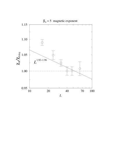
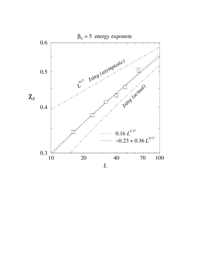
Figure 9: Left: the magnetic susceptibility $\chi_{M}$ divided by the Ising scaling law $\mbox{const}\times L^{1.96}$. The corresponding critical exponent is $\gamma/\nu=1.92(3)$, whereas Ising model has $\gamma/\nu=2-\eta\approx 1.96$. It is seen that at larger volumes the results for $\chi_{M}$ are consistent with the Ising model. The absolute value of $\chi_{M}$ is $\sim 5\times 10^{4}$ at $L=64$. Right: the energy susceptibility $\chi_{E}$. Note that the absolute value is much smaller than for $\chi_{M}$. Two different fits to the datapoints are shown. It is seen that the behaviour is consistent with that of the Ising model (which is described by $\chi_{E}=-11.1+14.6L^{0.17}$ [13] and is shown here up to an arbitrary overall factor, so only its slope is relevant). O(N) models with $N\geq 2$ have a negative exponent for $\chi_{E}$ and are thus excluded.

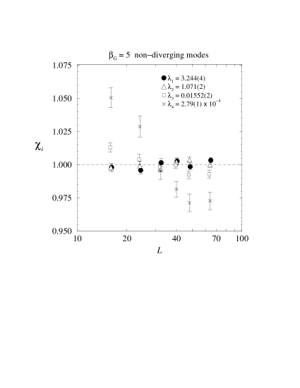
Figure 10: The regular eigenvalues, divided by the volume, as a function of the lattice size. The normalization is arbitrarily chosen such that the average of the values shown is 1.0; the absolute values are as indicated by the numbers. It is seen that the eigenvalues are constant with a very good accuracy (note the scale of the $y$-axis). The smallest eigenvalue has the largest volume dependence as it is contaminated by higher states.

5.3 Critical indices

Now that the $M$- and $E$-like directions have been determined, one can find the critical indices, using the finite size scaling formulas in Eq. (16). The scaling has to be studied at the infinite volume critical point $x_{c}(\infty)$, whose determination was discussed in Sec. 5.1. There is a small dependence of eigenvectors on the lattice size, due to corrections to scaling; we take a fixed set of eigenvectors (corresponding to the largest lattice, $64^{3}$) and compute the second moments of the corresponding projections, for a set of lattice sizes. The dispersion of $M$ grows approximately as $L^{4.92}$, the dispersion of $E$ grows as $L^{3.27}$, and those of the remaining projections grow as $L^{3}$, as shown in Figs. 9, 10. (An additional volume factor enters due to observables being sums over the lattice, without dividing by the volume). The apparent value of $\alpha/\nu\approx 0.27$ deviates notably from the Ising asymptotic value 0.17, but just the same effect is observed for the Ising model itself, for similar lattice sizes. This is explained by the presence of a negative regular background in $\chi_{E}$ [13], as shown in Fig. 9.

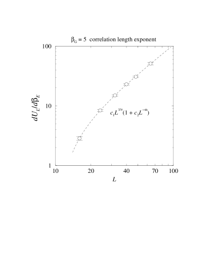
Figure 11: The slope of the Binder cumulant $U_{L}$ at the critical point in the $E$-like direction versus the lattice size. The dashed line is a 4-parameter fit to the data.

In addition to the critical exponents $\gamma/\nu$ and $\alpha/\nu$, which are related to the second moments of the distributions $P(M)$ and $P(E)$, we have also determined the correlation length critical exponent $\nu$. In models with an exact symmetry $M\leftrightarrow-M$ (like the Ising model), finite observables like the Binder cumulant

$$U_{L}\equiv 1-{\frac{1}{3}}{\frac{\langle M^{4}\rangle}{\langle M^{2}\rangle^{2}}}$$ (23)

can be assumed, near the critical point, to be regular functions of $\xi/L$, the ratio of the correlation length to the system size. As $\xi\sim t^{-\nu}$, the exponent $\nu$ can be obtained from the slope of $U_{L}$ at the critical point [30]:

$${\frac{\partial U_{L}}{\partial t}}\propto L^{1/\nu}\,.$$ (24)

The SU(2)+Higgs theory lacks the explicit $M\leftrightarrow-M$ -symmetry, and we use the $M$- and $E$-like eigenvectors in the analysis. Furthermore, we substitute $M\rightarrow\Delta M=M-\langle M\rangle$ in the Binder cumulant. Let us now denote by $\beta_{E}$ the coupling constant of the $E$-like eigenvector: that is, we formally extend the lattice action in Eq. (2) to the form $S+\beta_{E}E$, where $\beta_{E}=0$ at the critical point. We then obtain from Eqs. (23) and (24) that

$${\frac{\partial U_{L}}{\partial\beta_{E}}}=(1-U_{L})\left[\langle E\rangle+{\frac{\langle(\Delta M)^{4}E\rangle}{\langle(\Delta M)^{4}\rangle}}-2{\frac{\langle(\Delta M)^{2}E\rangle}{\langle(\Delta M)^{2}\rangle}}\right]\,.$$ (25)

This expression is readily evaluated using the $M$- and $E$-like eigenvectors at the critical point. The results are shown in Fig. 11. With these volumes the corrections to scaling are still substantial, and the points do not fall on a straight line on a log-log plot.

Taking into account the corrections to scaling, we fit the data with the 4-parameter ansatz

$${\frac{\partial U_{L}}{\partial\beta_{E}}}=c_{1}\,L^{1/\nu}\,\left(1-c_{2}\,L^{-\omega}\right)\,.$$ (26)

However, with only 6 points and relatively large statistical errors (when compared with, say, the Ising model simulations [28]) the error range in the correlation length critical exponent becomes rather large: the result is $\nu=0.63(17)$. If we lock the correction to scaling exponent $\omega$ to the central value $\omega=1.7$ and perform a three-parameter fit, the result becomes $\nu=0.63(3)$.

The value of $\nu$ is completely compatible with the Ising model (but also with O(2)). However, in the Ising model the correction to scaling exponent is $\omega=0.8$, which does not fit the data well. This is very likely due to the asymmetry in the $P(M,E)$-distributions of the smallest volumes (Fig. 5). In order to observe the Ising-type corrections to scaling one should use volumes which are large enough so that the asymmetric corrections to scaling have become subdominant. This is discussed in more detail in the next section.

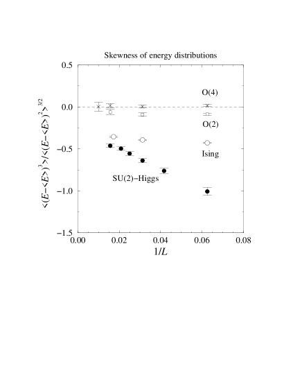
Figure 12: The skewness of $P(E)$ for 3d SU(2)+Higgs and different spin models, versus the inverse lattice size.

Apart from the second moments $\chi_{E}$, $\chi_{M}$, we have also measured the third moment of $E$ and the corresponding skewness ratio in Eq. (19). The results are shown in Fig. 12. They are consistent with those of the Ising model, but differ from O(2) and especially from O(4), in which case the skewness of $P(E)$ is very small.

6 Dependence of asymmetry on the volume

Significant asymmetry effects were observed in the previous analysis of the SU(2)+ Higgs theory. Here we study them in some more detail. We consider the distributions $P(M)$ at the critical point, as shown in Fig. 5(right), and attempt to obtain a quantitative description of how they approach the Ising shape with growing lattice size.

It is well-known [32] that the leading corrections to scaling in an exactly symmetric system, such as the Ising model itself, show the universal behaviour governed by $L^{-\omega}$, $\omega\equiv\Delta/\nu\approx 0.8$ (see also Sec. 5.1). However, the asymmetric corrections, which are also present in our system, have their own critical exponent $\omega_{5}$, which is different from $\omega$ and has attracted much less attention in the literature (to our knowledge, it has never been studied before in the framework of Monte Carlo simulations). Including the operators $\phi^{5},\phi^{6}$ in Eq. (10), the exponent $\omega_{5}$ has been computed within the $\varepsilon$-expansion up to order $\varepsilon^{3}$ [33]–[35], and within the renormalization group framework [36]. Quoting from [35],

$$\omega_{5}=1+{11\over 6}\varepsilon-{685\over 324}\varepsilon^{2}+{107855+103680\zeta(3)\over 34992}\varepsilon^{3}+O(\varepsilon^{4}).$$ (27)

This series behaves poorly at $\varepsilon=1$, resulting in $1+1.83-2.11+6.64\ldots$. An attempt to improve the situation using Padé approximants produces the sequence 2.83, 1.85, 2.32, in orders $O(\varepsilon)$, $O(\varepsilon^{2})$, $O(\varepsilon^{3})$ respectively, leading to the estimate that $\omega_{5}\mathop{\raise 1.29167pt\hbox{$>$\kern-7.5pt\raise-4.73611pt\hbox{$\sim$}}}1.5$ [35]. This estimate has been confirmed by the computation within the renormalization group [36], which resulted in $\omega_{5}=2.4(5)$. Thus it is generally believed (see, e.g., [37]), that $\omega_{5}\approx 2.1$ (the average of the last two Padé values). This implies that the asymmetric corrections, going as $L^{-\omega_{5}}$, should die out very rapidly when a critical point is approached, not only faster than the leading symmetric corrections $(L^{-\omega})$, but also faster than the subleading ones $(L^{-2\omega})$, and thus be of no practical importance anywhere near the critical point. This is probably the reason why $\omega_{5}$ is rarely discussed in the literature.

However, we do observe significant asymmetric contributions, and it is interesting to see what kind of implications there are for $\omega_{5}$. For this purpose we need to quantify the deviation of $P(M)$ from the Ising scaling form (Fig. 5, right). As has been found in [31], the scaling form of $P(M)$ for the 3d Ising model in a cubic box with periodic boundary conditions is described extremely well by the following simple approximation:

$$P(M)\propto\exp\biggl{\{}-\biggl{(}{M^{2}\over M_{0}^{2}}-1\biggr{)}^{2}\biggl{(}a{M^{2}\over M_{0}^{2}}+c\biggr{)}\biggr{\}},$$ (28)

where $M_{0}$ is the position of the magnetization peak, and the universal constants $a$ and $c$ are

$$a = 0.158(2),$$ (29)

$$c = 0.776(2).$$

The generalization of Eq. (28) for our case must also include odd powers of $M$, and can be written down as follows:

$$P(M)\propto e^{-V_{\mbox{\scriptsize eff}}},\quad V_{\mbox{\scriptsize eff}}=(x^{2}-1)^{2}(ax^{2}+bx+c)-hx,\quad x=\frac{M-M_{1}}{M_{0}}.$$ (30)

This $V_{\mbox{\scriptsize eff}}$ can be considered as a special parametrization of a general double-well polynomial of up to sixth order in $M$. The parameters $M_{0}$ and $M_{1}$ are responsible for rescaling and shifting the distribution as a whole. Two of the remaining four parameters, $b$ and $h$, characterize the asymmetry of $P(M)$.

One of them, $h$, is sensitive to what may be called the superficial asymmetry: an asymmetry caused by a small deviation of parameters of our system from the true critical point across the first order line, which is, in the case of the Ising model, equivalent to an application of a small external field. This parameter is also sensitive to the asymmetry caused by statistical errors in the relative heights of the two peaks, which emerge on larger lattices as a consequence of the growth of the tunnelling time with the lattice size.

On the other hand, the parameter $b$ characterizes what may be called the genuine asymmetry, and is responsible for the difference in the peak widths that remains after we make them equally high by slightly shifting the system across the phase transition line (that is, in the $h$-like direction).

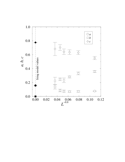
Figure 13: The parameters $a$, $b$, $c$ that determine the shape of $P(M)$ according to Eq. (30), as a function of the lattice size ($L=16\ldots 64$). The values in Eq. (29) for the Ising model in the scaling limit are marked on the left edge of the plot.

Thus we will be interested in three parameters: $a$, $b$ and $c$. Making a 6-parameter fit to our data, we observe (Fig. 5, right) that the ansatz in Eq. (30) is indeed able to provide a sufficiently good approximation. The quality of the approximation turns out not to be exactly as excellent as in the case of the 3d Ising model (one observes, for example, that the fit tends to go a little bit above the top of the higher peak), but quite sufficient for our purposes.

The results for $a$, $b$ and $c$ are shown in Fig. 13. One observes that all three parameters go in the directions of the corresponding Ising limits, with growing lattice size.

The parameter $c$ falls reasonably well on a straight line which corresponds to the standard correction to the scaling exponent $\omega\approx 0.8$. It is interesting to note that it approaches the scaling limit from below, while in the simple cubic Ising model it approaches the same limit from above [31].

The parameter $a$ behaves less nicely but is also consistent with $\omega\approx 0.8$ for larger lattice sizes. As for the parameter $b$, which is expected to behave as $L^{-\omega_{5}}$, it does indeed decrease with growing lattice size, but much more slowly than implied by the generally accepted high value of $\omega_{5}$. In fact, $b$ seems to go down more slowly than $L^{-0.8}$, rather than going as $L^{-2.1}$ (the data in Fig. 13 are best fitted by $L^{-0.4}\ldots L^{-0.5}$)!

The origin of this contradiction remains unclear. It might be that our lattices are still too small, and we have not yet reached the asymptotic regime where asymmetric corrections behave as $L^{-\omega_{5}}$. On the other hand, something might be missing in the theoretical treatment of asymmetric corrections to scaling. This question certainly deserves further study.

7 Summary of the results

The aim of this paper was to study the universality properties of the endpoint of the line of first order phase transitions in the 3d SU(2)+Higgs gauge theory. Qualitatively, the result was obvious when comparing the two-dimensional near-endpoint distribution of this theory in E- and M-like variables, shown in Fig. 2(b), with the corresponding distribution for the 3d Ising model shown in Fig. 2(c): the distributions look extremely similar. The bulk of this paper was devoted to putting this similarity on a strict quantitative basis.

Indeed, the two main discrepancies between Figs. 2(b) and 2(c) – the asymmetry and the thickness of Fig. 2(b) – can be removed by going to the infinite volume limit and by using a larger basis of observables. The effect of the volume variations is shown in Fig. 5. It is seen that as the volume is increased, the distribution looks more and more like that of the Ising model, Fig. 3(a). The effect of the choice of basis is shown in Fig. 7. It is seen that the thickness is removed as one goes from two to four observables, and even more as one goes to six observables (Fig. 5(c)). The fact the Fig. 5(c) agrees with Fig. 3(a) and not with Figs. 3(b),(c), is our main result.

Furthermore, the basis of six observables allows to construct a $6\times 6$ correlation matrix, which is then diagonalized. It turns out that two of the eigenvalues show critical behaviour, whereas four are regular. The largest eigenvalue corresponds to $\chi_{M}$. The susceptibilities $\chi_{M},\chi_{E}$ are shown in Fig. 9 as a function of the volume. The behaviour is clearly consistent with that of the Ising model. For the energy exponent $\chi_{E}$ even the fact that scaling violations are large at moderate volumes is reproduced. An O(4) model with a negative exponent for $\chi_{E}$ is excluded.

The remaining four regular exponents are shown in Fig. 10. They show no critical behaviour as a function of the volume.

Apart from the second moments $\chi_{E},\chi_{M}$, we have measured the correlation length critical exponent $\nu$ (Fig. 11) and the skewness of $P(E)$ (Fig. 12). The results are completely consistent with those of the Ising model.

Based on the values of the critical exponents and properties of $P(M,E)$, $P(M)$ and $P(E)$, we thus conclude that the endpoint of the SU(2)+Higgs theory is in the universality class of the 3d Ising model.

We have also studied corrections to scaling. While “symmetric” corrections to scaling display precisely the exponent inherent for the 3d Ising model (Sec. 5.1), asymmetric corrections to scaling, which arise from higher order operators not appearing in the actions in Eqs. (10), (11), behave in an unexpected way: they are quite large at reasonable lattice sizes.

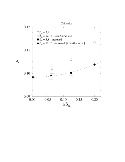
Figure 14: The infinite volume extrapolations of $x_{c}$ as a function of $\beta_{G}$. Gürtler et al refers to [3]. The location of the endpoint has been determined in [2], as well, but the volumes there were somewhat smaller so that the inclusion of that datapoint is not meaningful. The improved values have been obtained from Eq. (9).

7.1 The continuum limit of $x_{c}$

Finally, let us discuss the continuum limit of $x_{c}$, the location of the endpoint, which is a non-universal quantity. This requires measurements performed at different lattice spacings; for $\beta_{G}=8$ we used a set of simulations originally described in [1], and for $\beta_{G}=12$ we used the critical coupling measured in [3]. The results are shown in Fig. 14. The improved values for $x_{c}$ have been obtained from Eq. (9). As the corrections linear in $1/\beta_{G}$ are thus removed, a quadratic extrapolation can be made. The continuum result is

$$x_{c}=0.0983(15).$$ (31)

We estimate that the effect of the U(1) group on $x_{c}$ is $\mathop{\raise 1.29167pt\hbox{$<$\kern-7.5pt\raise-4.73611pt\hbox{$\sim$}}}10$%. According to the formulas in [7], the value of $x_{c}$ in Eq. (31) corresponds to $m_{H}=72(2)$ GeV in the SM, and $x_{c}=0.11$ would correspond to $m_{H}=77(2)$ GeV. In the MSSM, the same effective theory as in Eq. (1) can be derived, just the relations to 4d parameters are different [19]. Then the value $x=x_{c}$ can correspond to many different Higgs masses, depending on the other parameters of the theory: some examples are shown in Fig. 15.

Figure 15: Examples of parameter values corresponding to $x=x_{c}$ in the MSSM [38]. Here $m_{\tilde{t}_{R}}$ is the right-handed stop mass, $m_{H}$ is the lightest CP-even Higgs mass and $m_{A}$ is the CP-odd Higgs mass. The squark mixing parameters have been put to zero.

8 Conclusions

In this paper, we have shown that the endpoint of the line of first order transitions in the 3d SU(2)+Higgs theory is a second order transition in the universality class of the 3d Ising model. In particular, the measured critical exponents, cumulant ratios, and probability distributions of these two theories approach each other with growing lattice size.

To arrive at this conclusion, we have developed a general method to determine the universality class of a phase transition in a completely non-perturbative system, utilizing lattice Monte Carlo simulations. The method can be applied to any system exhibiting critical behaviour, provided that it is possible to perform Monte Carlo simulations on the critical point itself. This includes, e.g., the endpoints of the 1st order lines in the 3d SU(2)+adjoint Higgs theory (where the line ends [39, 40]), the 3d SU(3)+adjoint Higgs theory (where the line turns into a second order line after a tricritical point) or in the U(1)+Higgs theory. On the other hand, the two flavour 4d finite temperature chiral transition in QCD occurs at the limit $m_{q}\rightarrow 0$, which is not directly accessible with standard Monte Carlo methods.

We have also determined the continuum extrapolation of an important non-universal quantity, the location of the endpoint $x_{c}$. In the Standard Model with $\sin^{2}\theta_{W}=0$, the resulting value $x_{c}=0.0983(15)$ corresponds to a physical Higgs mass $m_{H}=72(2)$ GeV. While taking $\sin^{2}\theta_{W}=0.23$ does not change the universal properties, the value of $x_{c}$ may grow slightly. However, we do not expect values larger than $x_{c}=0.11$, corresponding to $m_{H}=77(2)$ GeV. Even this Higgs mass is already excluded experimentally, and thus there is no phase transition in the Standard Model. If low energy supersymmetry is realized, in contrast, the cosmological electroweak phase transition can be of the first order for the Higgs masses allowed at present. This could lead to important cosmological consequences.

Appendix

In this appendix we discuss two points concerning the scalar effective theory in Eq. (10): the relative roles of the linear and cubic terms and discretization. The cubic term is often used to generate a first order transition, but here it proves convenient to shift it away.

Consider the theory

$$S=\int\!d^{3}x\biggl{[}{\frac{1}{2}}\partial_{i}\phi\partial_{i}\phi+h\phi+{\frac{1}{2}}m^{2}\phi^{2}-{\frac{1}{3}}\delta\phi^{3}+{\frac{1}{4}}\lambda\phi^{4}\biggr{]}.$$ (32)

Due to superrenormalisability, only the two 2-loop diagrams

are logarithmically divergent and lead to the following renormalisation scale dependence of the mass and magnetic field terms in the $\overline{\mbox{\rm MS}}$ scheme:

$$h(\mu)={2\lambda\delta\over 16\pi^{2}}\log{\Lambda_{h}\over\mu},\quad m^{2}(\mu)={-6\lambda^{2}\over 16\pi^{2}}\log{\Lambda_{m}\over\mu}.$$ (33)

The theory now is specified by the four constants $\lambda,\delta,\Lambda_{h},\Lambda_{m}$ or, equivalently, by

$$\lambda,\quad x={m^{2}(\lambda)\over\lambda^{2}},\quad y={h(\lambda)\over\lambda^{5/2}},\quad z={\delta\over\lambda^{3/2}}.$$ (34)

However, as there is no $\phi\leftrightarrow-\phi$ symmetry, one can perform a shift $\phi\to\phi+$constant and choose the constant so that the cubic term disappears. This corresponds to the invariance of the theory under the transformation $(x,y,z)\to(x+zy/3-2z^{3}/27,y-z^{2}/3,0)$. Thus one can from the outset choose $\delta=0$ in Eq. (32). The magnetic field term is then scale invariant (see Eq. (33)). However, it is not possible to eliminate the linear term: it is anyway generated by radiative effects according to Eq. (33).

On the lattice the action corresponding to the theory without the cubic term becomes (after scaling $a\phi^{2}\to\beta_{H}\phi^{2}$)

$$S = -\beta_{H}\sum_{{\bf x},i}\phi({\bf x}+i)\phi({\bf x})+\beta_{1}\sum_{\bf x}\phi({\bf x})$$ (35)

$$+\sum_{\bf x}\phi^{2}({\bf x})+{\beta_{H}^{2}\over 4\beta_{G}}\sum_{\bf x}[\phi^{2}({\bf x})-1]^{2},$$

where the lattice couplings $\beta_{H},\beta_{G},\beta_{1}$ are related to $\lambda a,x,y$ by

$$\lambda a = {1\over\beta_{G}},$$

$$x = 2\beta_{G}^{2}\biggl{(}{1\over\beta_{H}}-3-{\beta_{H}\over 2\beta_{G}}\biggr{)}+{3\Sigma\over 4\pi}\beta_{G}-{6\over 16\pi^{2}}\log(6\beta_{G}+\zeta),$$ (36)

$$y = {\beta_{1}\over\sqrt{\beta_{H}}}\beta_{G}^{5/2}.$$

Here $\Sigma,\zeta$ are the same as in Eq. (7). Eq. (35) is a standard scalar lattice action but with very specific couplings, determined by Eqs. (36). If the expectation value of $\phi$ measured with Eq. (35) is $\langle\phi_{L}\rangle$, then in continuum normalisation,

$$\langle\phi\rangle/\lambda^{1/2}=\sqrt{\beta_{H}\beta_{G}}\langle\phi_{L}\rangle.$$ (37)

If higher order operators are included in Eq. (32), then the cubic term cannot, in general, be shifted away any more. It becomes a running parameter which is generated radiatively even if shifted away at some scale.

References

- [1] K. Kajantie, M. Laine, K. Rummukainen and M. Shaposhnikov, Phys. Rev. Lett. 77 (1996) 2887 [hep-ph/9605288].
- [2] F. Karsch, T. Neuhaus, A. Patkós and J. Rank, Nucl. Phys. B (Proc. Suppl.) 53 (1997) 623 [hep-lat/9608087].
- [3] M. Gürtler, E.-M. Ilgenfritz and A. Schiller, Phys. Rev. D 56 (1997) 3888 [hep-lat/9704013]; M. Gürtler, E.-M. Ilgenfritz, A. Schiller and G. Strecha, Nucl. Phys. B (Proc. Suppl.) 63 (1998) 563 [hep-lat/9709020].
- [4] W. Buchmüller and O. Philipsen, Nucl. Phys. B 443 (1995) 47 [hep-ph/9411334].
- [5] The Aleph Collaboration, ALEPH 98-029, 26 March 1998.
- [6] P. Ginsparg, Nucl. Phys. B 170 (1980) 388; T. Appelquist and R. Pisarski, Phys. Rev. D 23 (1981) 2305.
- [7] K. Kajantie, M. Laine, K. Rummukainen and M. Shaposhnikov, Nucl. Phys. B 458 (1996) 90 [hep-ph/9508379]; Phys. Lett. B, in press [hep-ph/9710538].
- [8] K. Jansen, Nucl. Phys. B (Proc. Suppl.) 47 (1996) 196 [hep-lat/9509018].
- [9] K. Rummukainen, Nucl. Phys. B (Proc. Suppl.) 53 (1997) 30 [hep-lat/9608079].
- [10] K. Kajantie, M. Laine, K. Rummukainen and M. Shaposhnikov, Nucl. Phys. B 466 (1996) 189 [hep-lat/9510020].
- [11] K. Kajantie, M. Laine, K. Rummukainen and M. Shaposhnikov, Nucl. Phys. B 493 (1997) 413 [hep-lat/9612006].
- [12] For a recent quantitative study of the 3d Ising model, see M. Caselle and M. Hasenbusch, J. Phys. A 30 (1997) 4963 [hep-lat/9701007].
- [13] M. Hasenbusch and K. Pinn, HUB-EP-97/29 [cond-mat/9706003].
- [14] K. Kanaya and S. Kaya, Phys. Rev. D 51 (1995) 2404 [hep-lat/9409001].
- [15] D. Toussaint, Phys. Rev. D 55 (1997) 362 [hep-lat/9607084].
- [16] F. Karsch, T. Neuhaus, A. Patkós and J. Rank, Nucl. Phys. B 474 (1996) 217 [hep-lat/9603004].
- [17] J.L. Alonso et al, Nucl. Phys. B 405 (1993) 574 [hep-lat/9210014].
- [18] A.D. Bruce and N.B. Wilding, Phys. Rev. Lett. 68 (1992) 193; N.B. Wilding and A.D. Bruce, J. Phys.: Cond. Mat. 4 (1992) 3087; N.B. Wilding, Phys. Rev. E 52 (1995) 602 [cond-mat/9503145]; N.B. Wilding and M. Müller, J. Chem. Phys. 102 (1995) 2562 [cond-mat/9410077]; N.B. Wilding, J. Phys.: Cond. Mat. 9 (1997) 585 [cond-mat/9610133].
- [19] M. Laine, Nucl. Phys. B 481 (1996) 43; J.M. Cline and K. Kainulainen, Nucl. Phys. B 482 (1996) 73; Nucl. Phys. B 510 (1997) 88; M. Losada, Phys. Rev. D 56 (1997) 2893; G.R. Farrar and M. Losada, Phys. Lett. B 406 (1997) 60.
- [20] K. Farakos, K. Kajantie, K. Rummukainen, and M. Shaposhnikov, Nucl. Phys. B 442 (1995) 317 [hep-lat/9412091]; M. Laine, Nucl. Phys. B 451 (1995) 484 [hep-lat/9504001]; M. Laine and A. Rajantie, Nucl. Phys. B 513 (1998) 471 [hep-lat/9705003].
- [21] G.D. Moore, Nucl. Phys. B 493 (1997) 439; McGill-97-23 [hep-lat/9709053].
- [22] A. Jakovác, K. Kajantie and A. Patkós, Phys. Rev. D 49 (1994) 6810; A. Jakovác and A. Patkós, Phys. Lett. B 334 (1994) 391.
- [23] F. Karsch, T. Neuhaus and A. Patkós, Nucl. Phys. B 441 (1995) 629 [hep-lat/9406012].
- [24] J.J. Rehr and N.D. Mermin, Phys. Rev. A 8 (1973) 472.
- [25] J. Zinn-Justin, Quantum Field Theory and Critical Phenomena, 2nd ed. (Oxford University Press, Oxford, 1993).
- [26] H.G. Ballesteros et al, Phys. Lett. B 387 (1996) 125 [cond-mat/9606203]; P. Butera and M. Comi, Phys. Rev. B 52 (1995) 6185 [hep-lat/9505027]; Phys. Rev. B 56 (1997) 8212 [hep-lat/9703018].
- [27] R. Guida and J. Zinn-Justin, SPhT-t97/40 [cond-mat/9803240].
- [28] M. Hasenbusch, K. Pinn and S. Vinti, HUB-EP-98/26 [cond-mat/9804186].
- [29] H.W.J. Blöte, E. Luijten and J.R. Heringa, J. Phys. A: Math. Gen. 28 (1995) 6289 [cond-mat/9509016].
- [30] K. Binder, Z. Phys. B 43 (1981) 119.
- [31] M.M. Tsypin and H.W.J. Blöte, to appear.
- [32] F.J. Wegner, Phys. Rev. B 5 (1972) 4529.
- [33] F.J. Wegner, Phys. Rev. B 6 (1972) 1891.
- [34] J.F. Nicoll and R.K.P. Zia, Phys. Rev. B 23 (1981) 6157; J.F. Nicoll, Phys. Rev. A 24 (1981) 2203.
- [35] F.C. Zhang and R.K.P. Zia, J. Phys. A 15 (1982) 3303.
- [36] K.E. Newman and E.K. Riedel, Phys. Rev. B 30 (1984) 6615.
- [37] M.A. Anisimov, A.A. Povodyrev, V.D. Kulikov and J.V. Sengers, Phys. Rev. Lett. 75 (1995) 3146.
- [38] This figure is based on the results in the first of [19].
- [39] A. Hart, O. Philipsen, J.D. Stack and M. Teper, Phys. Lett. B 396 (1997) 217 [hep-lat/9612021].
- [40] K. Kajantie, M. Laine, K. Rummukainen and M. Shaposhnikov, Nucl. Phys. B 503 (1997) 357 [hep-ph/9704416].