Microscopic universality with dynamical fermions

Abstract

It has recently been demonstrated in quenched lattice simulations that the distribution of the low-lying eigenvalues of the QCD Dirac operator is universal and described by random-matrix theory. We present first evidence that this universality continues to hold in the presence of dynamical quarks. Data from a lattice simulation with gauge group SU(2) and dynamical staggered fermions are compared to the predictions of the chiral symplectic ensemble of random-matrix theory with massive dynamical quarks. Good agreement is found in this exploratory study. We also discuss implications of our results.

It was conjectured a few years ago [1, 2] that the microscopic spectral properties of the QCD Dirac operator, in particular the distribution of the low-lying eigenvalues, are universal and can be obtained in effective theories that are much simpler than QCD. This conjecture rests on the observation [3] that in the range $1/\Lambda\ll V^{1/4}\ll 1/m_{\pi}$, where $\Lambda$ is a typical hadronic scale, $V$ is the space-time volume, and $m_{\pi}$ is the pion mass, the mass dependence of the finite-volume partition function of QCD is completely determined by global symmetries. Thus, the spectral properties of the Dirac operator on the “microscopic” scale $\sim 1/(V\Sigma)$, where $\Sigma$ is the absolute value of the chiral condensate, can be computed in effective theories with only the global symmetries as input, such as the framework of effective Lagrangians [1] or chiral random-matrix theory (RMT) [2].

The global spectral density of the Euclidean Dirac operator $D\raisebox{1.0pt}{/}\hskip 1.0pt=\partial\raisebox{1.0pt}{/}\hskip 0.5pt+igA\raisebox{1.0pt}{/}\hskip 1.0pt$ is given by $\rho(\lambda)=\langle\sum_{n}\delta(\lambda-\lambda_{n})\rangle_{A}$, where the $\lambda_{n}$ are the eigenvalues of $iD\raisebox{1.0pt}{/}\hskip 1.0pt$ and the average is over all gauge field configurations $A$ weighted by $\exp(-S_{\rm QCD})$. The Banks-Casher formula, $\Sigma=\pi\rho(0)/V$ [4], relates the spectral density at zero virtuality to the chiral condensate. If chiral symmetry is spontaneously broken, this relation implies that the spacing of the low-lying eigenvalues is $\sim 1/(V\Sigma)$, rather than $\sim 1/V^{1/4}$ as in the case of the non-interacting Dirac operator. Thus, the distribution of the low-lying eigenvalues is of great interest for a better understanding of the phenomenon of spontaneous chiral symmetry breaking.

It has recently been shown that the microscopic spectral properties of the staggered lattice Dirac operator in quenched SU(2) are indeed universal and described by chiral RMT [5, 6]. However, for a better understanding of hadronic properties it is important to go beyond the quenched approximation. One of the problems that arises in unquenched lattice simulations is that one cannot go to arbitrarily small quark masses. An important point is how small the masses of the dynamical quarks have to be so that they are really dynamical, i.e., lead to results that are different from those obtained in the quenched approximation. In this context, the main question that will be addressed in this work is the following. What is the effect of light dynamical quarks with masses of order $\sim 1/(V\Sigma)$ on the low-lying spectrum of the Dirac operator, and can this effect be described by results obtained in chiral RMT? The answer to these questions together with the analytical information available from RMT leads to a better understanding of the mass and energy scales in the problem and has important technical implications with regard to extrapolations to various limits (chiral, thermodynamic, continuum) that are difficult to take on the lattice. Moreover, analytical knowledge of the distribution of the smallest eigenvalues may be interesting from an algorithmic point of view.

We will mainly be concerned with the distribution of the smallest positive eigenvalue, $P(\lambda_{\rm min})$, and with the microscopic spectral density, $\rho_{s}(z)$, defined by [2]

$$\rho_{s}(z)=\lim_{V\to\infty}\frac{1}{V\Sigma}\>\rho\left(\frac{z}{V\Sigma}\right)\>.$$ (1)

This definition amounts to a magnification of the region of low-lying eigenvalues by a factor of $V\Sigma$ and leads to the resolution of individual eigenvalues. The claim is that the quantities $P(\lambda_{\rm min})$ and $\rho_{s}(z)$ are universal (see Ref. [5] for a summary of existing evidence) and can be computed exactly in an effective theory. We will concentrate on chiral RMT although identical results could also be obtained from the finite-volume partition function computed from an effective Lagrangian [7, 8].

Let us recall how the random-matrix model is constructed. In a chiral basis, the weight function of full QCD with $N_{f}$ flavors can be written as

$$e^{-S_{\rm QCD}}=e^{-S_{\rm gl}}\prod_{f=1}^{N_{f}}\det\left[\matrix{m_{f}&iT\cr iT^{\dagger}&m_{f}}\right]\>,$$ (2)

where $S_{\rm gl}$ is the gluonic action, $T$ is a matrix representing $iD\raisebox{1.0pt}{/}\hskip 1.0pt$, and the $m_{f}$ are the masses of the dynamical quarks. We now replace $T$ by a random matrix $W$ with $N$ rows and $N+\nu$ columns ($|\nu|\ll N$). The dimensionless space-time volume can be identified with $2N$, and $\nu$ plays the role of the topological charge. The symmetry properties of $W$ depend on the gauge group and on the representation of the fermions  [9]. We will be concerned with staggered fermions in SU(2) for which the elements of $W$ are real quaternions. This is the chiral symplectic ensemble (chSE). The average over gauge field configurations is replaced by an average over random matrices, i.e., the factor $e^{-S_{\rm gl}}$ is replaced by a convenient distribution of the matrix $W$, often a simple Gaussian, but the results are insensitive to this choice [10, 11, 12]. For the present work, the second factor in Eq. (2) is more interesting. In terms of the eigenvalues of $W$, it reads for the chSE [9]

$$\prod_{f=1}^{N_{f}}\det(WW^{\dagger}+m_{f}^{2})\propto|\Delta(\lambda^{2})|^{4}\prod_{n}\lambda_{n}^{4\nu+3}\prod_{f=1}^{N_{f}}(\lambda_{n}^{2}+m_{f}^{2})$$ (3)

in a sector of topological charge $\nu$, where $\Delta$ is the Vandermonde determinant. Thus, in the random-matrix model the fermion determinants can be taken into account without further assumptions. From Eq. (3) it is intuitively clear that the presence of the fermion determinants will affect the microscopic spectral quantities only if the $m_{f}$ are on the order of the smallest eigenvalue or, in other words, on the order of the mean level spacing near zero [2, 13]. Thus, we require $m_{f}\sim 1/(V\Sigma)$ to observe an effect on $P(\lambda_{\rm min})$ and $\rho_{s}(z)$. For quark masses much larger than this, we should simply obtain agreement with the RMT-results computed in the quenched approximation. This was already observed in Ref. [14] where the lattice data of Ref. [15] were analyzed.

RMT-predictions for the microscopic spectral quantities in the presence of massive dynamical quarks have recently been computed for the chiral unitary ensemble [16, 17] (see also [13]) and the unitary ensemble [18]. However, we want to compare lattice data with random-matrix predictions for the chSE. In this case, closed analytical expressions are at present only known in the chiral limit [19, 20, 21]. Analytical work for the massive case is in progress, but in the meantime we have computed the RMT-predictions for the chSE with massive quarks numerically using the methods of Ref. [20]. Essentially, one has to do an iterative computation of skew-orthogonal polynomials which obey orthogonality relations determined by a weight function involving the fermion determinants. To avoid cancellation problems, we have used a multi-precision package [22]. The calculation was done with matrices $W$ of finite dimension $N$ up to $N=100$. The remaining finite-$N$ effects can be estimated from a calculation in the chiral limit and are on the order of 1%.

We now summarize some RMT-results for the chSE in the chiral limit which we will need in the following. With $\alpha=N_{f}+2|\nu|$, we have [20, 23, 6]

$$\rho_{s}(z) = z\left[J_{\alpha}^{2}(2z)-J_{\alpha+1}(2z)J_{\alpha-1}(2z)\right]$$ (5)

$$-\frac{1}{2}J_{\alpha}(2z)\int_{0}^{2z}dtJ_{\alpha}(t)\>,$$

where $J$ denotes the Bessel function. Rescaling $\lambda_{\rm min}$ by $V\Sigma$ as in Eq. (1), we have for $N_{f}=\nu=0$ [19]

$$P(\lambda_{\rm min})=\sqrt{\frac{\pi}{2}}\lambda_{\rm min}^{3/2}I_{3/2}(\lambda_{\rm min})\,e^{-\frac{1}{2}\lambda_{\rm min}^{2}}\>,$$ (6)

where $I$ is the modified Bessel function. Further analytical results for $P(\lambda_{\rm min})$ are known if $\alpha$ is odd, i.e., for odd $N_{f}$. For example, we have for $N_{f}=1$ and $\nu=0$ [21]

$$P(\lambda_{\rm min})=\frac{1}{2}\lambda_{\rm min}[2I_{2}(2\lambda_{\rm min})-I_{0}(2\lambda_{\rm min})+1]\,e^{-\frac{1}{2}\lambda_{\rm min}^{2}}\>.$$ (7)

We shall also need $P(\lambda_{\rm min})$ for $N_{f}=2$ and 4 which in the absence of closed analytical expressions can perhaps most easily be obtained from results computed by Kaneko [24]. The essential ingredients are the zonal polynomials at the symmetric point. We obtain after some algebra

$$P(\lambda_{\rm min})=\frac{2}{(\alpha+1)!(\alpha+3)!}\lambda_{\rm min}^{2\alpha+3}e^{-\frac{1}{2}\lambda_{\rm min}^{2}}T(\lambda_{\rm min}^{2})\>,$$ (8)

where $T(x)=1+\sum_{d=1}^{\infty}a_{d}\,x^{d}$ with

$$a_{d} = \sum_{{|\kappa|=d}\atop{l(\kappa)\leq\alpha+1}}\prod_{(i,j)\in\kappa}\frac{\alpha\!+\!2j\!-\!i}{\alpha\!+\!2j\!-\!i\!+\!4}$$ (10)

$$\;\times\,\frac{1}{[\kappa_{j}^{\prime}\!-\!i\!+\!2(\kappa_{i}\!-\!j)\!+\!1][\kappa_{j}^{\prime}\!-\!i\!+\!2(\kappa_{i}\!-\!j)\!+\!2]}\>.$$

Here, $\kappa$ denotes a partition of the integer $d$, $l(\kappa)$ its length, $|\kappa|$ its weight, and $\kappa^{\prime}$ the conjugate partition. In Eq. (10), a partition $\kappa$ is identified with its diagram, $\kappa=\{s=(i,j);1\leq i\leq l(\kappa),1\leq j\leq\kappa_{i}\}$. The Taylor series for $T(x)$ is rapidly convergent, and the curves for $N_{f}=2$ and 4 can easily be computed to any desired accuracy.

The RMT-results for $P(\lambda_{\rm min})$ and $\rho_{s}(z)$ are sensitive to the topological charge $\nu$. Thus, they are only universal in a given sector of topological charge. In the continuum limit, the overall result for a given quantity is a weighted average over these sectors. RMT can predict the quantity for definite $\nu$ but cannot predict the corresponding weights. In Ref. [5] it was found that for values of $\beta=4/g^{2}$ up to 2.4 the quenched SU(2) lattice data were consistent with $\nu=0$. Here, we only consider values of $\beta$ in the strong-coupling region, thus everything should be described by the RMT-results for $\nu=0$. We will not address the question of topology in the following.

Our lattice simulations were performed with gauge group SU(2) and staggered fermions on an $8^{4}$ lattice. The boundary conditions were periodic for the gauge fields and periodic in space and anti-periodic in Euclidean time for the fermions. A hybrid Monte Carlo algorithm [25, 26] was used to generate a large number of independent configurations. For the diagonalization of $-D\raisebox{1.0pt}{/}\hskip 1.0pt^{2}$ we have employed the Cullum-Willoughby version of the Lanczos algorithm [27]. The complete spectra where checked against the analytical sum rule ${\rm tr}(-D\raisebox{1.0pt}{/}\hskip 1.0pt^{2})=V$ for the distinct eigenvalues of $-D\raisebox{1.0pt}{/}\hskip 1.0pt^{2}$ [28]. All physical quantities will be quoted in units of the lattice spacing $a$, in contrast to Ref. [5] where the unit was $2a$.

The RMT-results contain one single parameter $V\Sigma$ which is determined by the lattice data via the Banks-Casher relation, $V\Sigma=\pi\rho(0)$. (Note that $\rho(\lambda)$ is normalized to $V$.) Thus, the random-matrix predictions are parameter-free. The simulation parameters and observables are summarized in Table I. We also give values for $\langle\bar{\psi}\psi\rangle(m)=(m/V)\sum_{\lambda_{n}>0}(\lambda_{n}^{2}+m^{2})^{-1}$. Note that we have $\mu=mV\Sigma\sim{\cal O}(1)$ as desired, where by ${\cal O}(1)$ we mean much smaller than $8^{4}=4096$.

TABLE I.: Simulation parameters and observables of our lattice calculations on an $8^{4}$ lattice. $\langle\bar{\psi}\psi\rangle(m)$ and $\Sigma$ are given in units of $a^{-3}$.

$\beta$	$\tilde{N}_{f}$	$ma$	conf.	$\langle\bar{\psi}\psi\rangle(m)$	$\Sigma$	$mV\Sigma$
1.8	4	0.015	1799	0.1517(14)	0.1250(46)	7.68
1.3	8	0.0075	1023	0.2669(12)	0.2846(38)	8.74
1.3	8	0.0055	1042	0.2470(11)	0.2800(45)	6.31
1.3	8	0.00375	703	0.2073(22)	0.2772(42)	4.26

Our results for $\beta=1.8$ and $\tilde{N}_{f}=4$ flavors of mass $ma=0.015$ are plotted in Fig. 1. Note that we have to compare the data with the RMT-predictions for $N_{f}=2$ in Eq. (3) for the following two reasons. First, because of the finite lattice constant the original ${\rm U}(4)\otimes{\rm U}(4)$ chiral symmetry of the (local) lattice action is broken down to ${\rm U}(1)\otimes{\rm U}(1)$. This would imply to use $N_{f}=1$ in Eq. (3). Second, because of a global charge conjugation symmetry which is special to SU(2) all eigenvalues are twofold degenerate. Equation (3) was derived for fermions in the adjoint representation, and the eigenvalues in the fermion determinants of Eq. (3) are assumed to be non-degenerate [9]. Therefore, the number of flavors must be doubled. Note that this is only an issue for SU(2). For these two reasons, we necessarily have to use $N_{f}=2$ in the random-matrix results.

After these comments, let us discuss Fig. 1. The presence of the fermion determinants leads to a suppression of small eigenvalues. The fact that the lattice data differ from the RMT-curves for the quenched approximation ($N_{f}=0$, or $\mu=\infty$) means that the dynamical quarks were light enough to affect the microscopic spectral quantities. However, the data are still closer to the RMT-curves for $N_{f}=0$ than to the ones for the chiral limit ($\mu=0$). This means that the dynamical quarks with a rescaled mass of $\mu=7.68$ are still quite heavy as far as the microscopic spectral properties are concerned. We will explore smaller masses in Fig. 2 below. The lattice data agree reasonably well with the random-matrix predictions for $N_{f}=2$ with the appropriate value of $\mu$. The systematic deviations and the question of the continuum limit will be discussed below and in the conclusions.

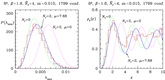
FIG. 1.: Distribution of the smallest eigenvalue (left) and microscopic spectral density (right) of the lattice Dirac operator for the simulation parameters indicated above the figures. The histograms represent the lattice data. The full lines are the RMT-predictions for $N_{f}=2$ and $\mu=mV\Sigma=7.68$, the dashed lines those for the quenched approximation, and the dotted lines those for $N_{f}=2$ in the chiral limit, respectively. Note that there is no free parameter involved.

For a larger number of flavors, the curves for the quenched approximation and those for the chiral limit are farther apart from each other so that the influence of massive dynamical quarks can be seen more easily. Therefore, we have also performed lattice simulations with $\tilde{N}_{f}=8$ flavors, shown in Fig. 2. A value of $\beta=1.3$ was chosen to ensure that we are in the broken phase for all values of the bare quark mass [26]. As expected from the above discussion, we have to compare the lattice data with the RMT-results for $N_{f}=4$ and the appropriate value of $mV\Sigma$. We see in Fig. 2 that, as the mass of the dynamical quarks is lowered, the lattice data move away from the quenched curves towards the RMT-curves computed in the chiral limit. This is precisely what we expect. Let us discuss the numbers. Our qualitative criterion was $\mu\sim{\cal O}(1)$. For $\mu=8.74$ (the top two figures in Fig. 2), we are still rather close to the quenched RMT-curves. For $\mu=4.26$ (the bottom two figures in Fig. 2), we are about half-way in between the quenched approximation and the chiral limit. We can now say more quantitatively that values of $\mu$ around 10 yield results which are close to those obtained in the quenched approximation, whereas values of $\mu$ smaller than 4 yield results which are closer to those obtained in the chiral limit. The mass scale on which dynamical quarks affect the microscopic spectrum of the Dirac operator is thus identified quantitatively.

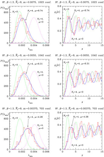
FIG. 2.: Same as Fig. 1 but for different simulation parameters (indicated above the figures).

In Fig. 3, we compare the data for $P(\lambda_{\rm min})$ computed for $\tilde{N}_{f}=8$ and the lightest quark mass, $m=0.00375$, with the RMT-predictions for various numbers of flavors and the appropriate value of $\mu$. The fact that the data agree well with the RMT-result for $N_{f}=4$ supports the two arguments made in connection with Fig. 1. In the continuum limit, one would expect agreement with the RMT-curve for $N_{f}=16$.

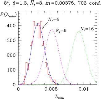
FIG. 3.: Distribution of the smallest eigenvalue for $\tilde{N}_{f}=8$ and $m=0.00375$ (histogram) compared with the RMT-predictions for various numbers of flavors (indicated in the figure) and $\mu=4.26$.

The agreement between the various lattice data and the RMT-predictions is not perfect. There are some systematic deviations which we believe to be largely due to the finite size of the lattice. Similar finite-size effects were observed in Ref. [5]. The present exploratory study was restricted to a relatively small lattice size since a large number of independent configurations is needed. One also observes from the figures that the agreement with RMT is better for smaller values of $\mu$, as expected from the discussion in the introduction. While it would be desirable to perform a comprehensive study for larger lattices and a number of different values of $\beta$, $N_{f}$, and $m$, the agreement between lattice data and random-matrix results seen in our figures is already very encouraging. We point out again that there is no free parameter involved. Another possibility would have been to fit the lattice data to the RMT-results by adjusting the parameter $V\Sigma$. This is an alternative way of determining the chiral condensate which also seems to eliminate some finite-size effects [23]. In this case, the agreement in Figs. 1 and 2 would have been better. However, the primary purpose of this work is the demonstration of parameter-free agreement between lattice data and RMT-predictions. This is the reason why we determined $\Sigma$ from $\rho(0)$ and not from a fit to RMT.

To conclude, we comment on the implications of our finding that lattice data for the small eigenvalues of the Dirac operator are described by chiral RMT also in the presence of dynamical quarks of mass $\sim 1/(V\Sigma)$. First of all, as far as the microscopic spectral properties are concerned, the dynamical quarks are only really dynamical if their masses are not much larger than $1/(V\Sigma)$. This provides information on the relevant mass scales in unquenched lattice simulations. Once the applicability of chiral RMT to full QCD with massive dynamical quarks is firmly established, one can address practical applications. For quantities which are sensitive to the small eigenvalues, the analytical RMT-results can provide guidance for extrapolations to the chiral limit. Also, as demonstrated in Ref. [23], extrapolations to the thermodynamic limit are facilitated since the RMT-results are derived in the limit $V\to\infty$. Another interesting aspect which deserves further investigation is the continuum limit where the original chiral symmetry of the action is restored and agreement with the RMT-results for the original number of flavors is expected. This might give an indication of how close to the continuum limit one actually is. However, much larger lattices are required to study such a transition. Moreover, we hope that the microscopic universality can perhaps be used in the development of hybrid fermionic algorithms that take into account the available analytical information. It would also be of great interest to extend our analysis to gauge group SU(3) where analytical RMT-results are already known. Finally, we hope to obtain analytical results for the chSE with massive dynamical quarks in the near future.

It is a pleasure to thank M. Göckeler, P. Rakow, A. Schäfer, J.J.M. Verbaarschot, and H.A. Weidenmüller for useful discussions. We also thank the MPI für Kernphysik, Heidelberg, for hospitality and support. This work was supported in part by DFG grant We 655/11-2. The numerical simulations were done on a CRAY T3E-900 at the HLRS Stuttgart.

REFERENCES

- [1] H. Leutwyler and A.V. Smilga, Phys. Rev. D 46 (1992) 5607.
- [2] E.V. Shuryak and J.J.M. Verbaarschot, Nucl. Phys. A 560 (1993) 306.
- [3] J. Gasser and H. Leutwyler, Phys. Lett. B 188 (1987) 477.
- [4] T. Banks and A. Casher, Nucl. Phys. B 169 (1980) 103.
- [5] M.E. Berbenni-Bitsch, S. Meyer, A. Schäfer, J.J.M. Verbaarschot, and T. Wettig, Phys. Rev. Lett. 80 (1998) 1146.
- [6] J.-Z. Ma, T. Guhr, and T. Wettig, Euro. Phys. J. A 2 (1998) 87.
- [7] A. Smilga and J.J.M. Verbaarschot, Phys. Rev. D 51 (1995) 829.
- [8] P.H. Damgaard, Phys. Lett. B 424 (1998) 322; G. Akemann and P.H. Damgaard, hep-th/9801133 and hep-th/9802174.
- [9] J.J.M. Verbaarschot, Phys. Rev. Lett. 72 (1994) 2531.
- [10] S. Nishigaki, Phys. Lett. B 387 (1996) 139; G. Akemann, P.H. Damgaard, U. Magnea, and S. Nishigaki, Nucl. Phys. B 487 (1997) 721.
- [11] M.K. Şener and J.J.M. Verbaarschot, hep-th/9801042, to appear in Phys. Rev. Lett.
- [12] S. Nishigaki, P.H. Damgaard, and T. Wettig, hep-th/9803007, to appear in Phys. Rev. D.
- [13] J. Jurkiewicz, M.A. Nowak, and I. Zahed, Nucl. Phys. B 478 (1996) 605, B 513 (1998) 759.
- [14] J.J.M. Verbaarschot, Phys. Lett. B 368 (1996) 137.
- [15] S. Chandrasekharan and N. Christ, Nucl. Phys. B (Proc. Suppl.) 47 (1996) 527.
- [16] P.H. Damgaard and S.M. Nishigaki, Nucl. Phys. B 518 (1998) 495.
- [17] T. Wilke, T. Guhr, and T. Wettig, Phys. Rev. D 57 (1998) 6486.
- [18] P.H. Damgaard and S.M. Nishigaki, Phys. Rev. D 57 (1998) 5299.
- [19] P.J. Forrester, Nucl. Phys. B 402 (1993) 709.
- [20] T. Nagao and P.J. Forrester, Nucl. Phys. B 435 (1995) 401.
- [21] T. Nagao and P.J. Forrester, Nucl. Phys. B 509 (1998) 561.
- [22] D.H. Bailey, A Fortran-90 based multiprecision system, NASA Ames RNR Technical Report RNR-94-013.
- [23] M.E. Berbenni-Bitsch, A.D. Jackson, S. Meyer, A. Schäfer, J.J.M. Verbaarschot, and T. Wettig, Nucl. Phys. B (Proc. Suppl.) 63A-C (1998) 820.
- [24] J. Kaneko, SIAM J. Math. Anal. 24 (1993) 1086.
- [25] S. Duane, A.D. Kennedy, B.J. Pendleton, and D. Roweth, Phys. Lett. B 195 (1987) 216.
- [26] S. Meyer and B.J. Pendleton, Phys. Lett. B 241 (1990) 397.
- [27] J. Cullum and R.A. Willoughby, J. Comp. Phys. 44 (1981) 329.
- [28] T. Kalkreuter, Phys. Rev. D 51 (1995) 1305.