April 1998

We present a number of arguments relating magnetic disorder to center disorder, in pure Yang-Mills theory in D=3 and D=4 dimensions. In the case of the D=3 Georgi-Glashow model, we point out that the abelian field distribution is not adequatedly represented, at very large scales, by that of a monopole Coulomb gas. The onset of center disorder is associated with the breakdown of the Coulomb gas approximation; this scale is pushed off to infinity in the $QED_{3}$ limit of the 3D Georgi-Glashow model, but should approach the color-screening length in the pure Yang-Mills limit.

1 Introduction

The $Z_{N}$ center of an $SU(N)$ gauge group is associated with the confinement properties of of a pure gauge theory in a number of ways. It is well known that the finite temperature confinement/deconfinement transition can be regarded as the breaking of a global $Z_{N}$ symmetry in a volume with a compactified time direction. In addition, as shown by ’t Hooft [1], the VEV of a $Z_{N}$ vortex creation operator can be interpreted as an order parameter for confinement, dual to Wilson loops, in $SU(N)$ gauge theory. It was also suggested many years ago that “thick” $Z_{N}$ vortices are responsible for the area-law falloff of Wilson loops [1, 2, 3, 4, 5, 6, 7, 8, 9], and recently there have been a number of numerical investigations which support this idea [10, 11, 12].

The notion that confining (“magnetic”) disorder is center disorder may also be supported by some simple observations, presented in section 2, regarding the behavior of holonomy probability distributions in Yang-Mills theory. We point out that the holonomy distribution approaches a random distribution on the group manifold as loop size increases; however, the approach to the random distribution is far more rapid among the center elements than among elements of the coset. We also show, with the help of the lattice strong-coupling expansion, that while center elements within a large area fluctuate independently, this is not true of fluctuations in the coset for $D>2$ dimensions.

The 3D Georgi-Glashow model ($GG_{3}$) is interesting in this context for several reasons. The confinement mechanism in this theory is believed to be essentially that of compact $QED_{3}$, at least in some region of the coupling parameters; one therefore expects that confining disorder is $U(1)$ disorder. There is only one phase in $GG_{3}$, but there are two special limits: Compact $QED_{3}$ is obtained in the limit where the mass of the W-boson becomes infinite, while pure Yang-Mills theory ($YM_{3}$) is obtained in the limit where the adjoint scalar effectively decouples from the gauge field. Since the 3D Georgi-Glashow model interpolates smoothly between $QED_{3}$ and $YM_{3}$, a natural question to ask is what happens to center disorder in $GG_{3}$ as we move away in parameter space from the pure Yang-Mills limit.

This question is taken up in section 3, where we point out a qualitative difference between confinement in compact $QED_{3}$, and confinement in the 3D Georgi-Glashow model at large scales. In the case of compact $QED_{3}$, we show via saddlepoint methods that double-charged loops have twice the string-tension of single-charged loops, while for $GG_{3}$, the double (abelian) charged loops must ultimately be screened by massive W-bosons. As a consequence, the effective abelian theory corresponding to the 3D Georgi-Glashow model, obtained after integrating out the charged bosons, is not adequately represented by a Coulomb gas of ’t Hooft-Polyakov monopoles. Our main point is that the massive W-bosons of $GG_{3}$ are not just spectators whose effect on vacuum fluctuations, beyond the range $M_{W}^{-1}$, is negligible; in fact the W-bosons must strongly affect the vacuum distribution of abelian flux at large distance scales. At these large scales, it appears that confining disorder in $GG_{3}$, as in the pure Yang-Mills theory, is associated with $Z_{2}$ (rather than $U(1)$) disorder. In the $QED_{3}$ limit, the onset of $Z_{2}$ disorder is pushed off to infinity, while in the pure Yang-Mills limit, it roughly coincides with the onset color screening.

2 Confining Disorder as Center Disorder

A Wilson loop is understood as measuring the response of the vacuum to the introduction of heavy sources, but it can also be viewed as providing information about field fluctuations in the ground state, in the absence of external charges. Consider, in particular, a gauge theory with matter fields in the fundamental representation. The asymptotic perimeter-law falloff of the Wilson loop is explained by the binding of matter quanta to the external charge, forming a color singlet. On the other hand, imagine integrating out the matter fields, leaving an effective action involving only the gauge fields. It is then clear that the effect of the virtual matter fields is to modify the probability distribution of gauge-field fluctuations, such that confining configurations, which would normally induce an asymptotic area-law falloff in the loop, are suppressed.

In discussing the probability distribution of gauge fields, with or without the presence of matter fields, it will be helpful to introduce a gauge-invariant operator which is somewhat more general than a Wilson loop. Consider, for simplicity, a lattice pure-gauge theory with an SU(2) gauge group, and let $U(C)$ denote the path-ordered product of link variables along a closed loop $C$ (the holonomy). The expectation value

$$P_{C}[g] = <\delta[g,U]>=<\sum_{j}\chi_{j}[g]\chi_{j}[U(C)]>$$ (1)

$$= 1+\sum_{j\neq 0}W_{j}(C)\chi_{j}[g]$$

is the probability density, on the SU(2) group manifold, that the loop $U(C)$ equals the group element $g$. The sum over $j$ runs over group representations, the $\chi_{j}(g)$ are SU(2) group characters, and $W_{j}(C)=<\chi_{j}[U(C)]>$ is the VEV of the Wilson loop in representation $j$. As loop $C$ becomes large, this holonomy probability distribution approaches the random distribution, $P_{C}(g)\rightarrow 1$, and it will be useful to focus on the deviation of $P_{C}$, denoted $\tilde{P}_{C}[g]$, from the random distribution

$$\tilde{P}_{C}[g]=P_{C}[g]-1$$ (2)

Since $P_{C}[g]$ is gauge-invariant, it can only depend on the eigenvalues of the unitary matrix $g$, and $P_{C}$ has flat directions on the group manifold corresponding to $g\rightarrow g^{\prime}=ugu^{\dagger}$. In the particular case of $SU(2)$, $P_{C}$ only depends on $\mbox{Tr}(g)$, and we will be interested in how this dependence fades away as the loop $C$ becomes large.

A Wilson loop $W_{j}(C)$ can be thought of as a moment of the probability distribution $P_{C}(g)$. It is expected that, in $D=3$ and $D=4$ dimensions, planar Wilson loops have the asymptotic form

$$W_{j}(C)=\left\{\begin{array}[]{cl}\exp[-\sigma{\cal A}(C)-\mu_{j}{\cal P}(C)-c_{j}]&j=\mbox{half-integer}\cr\exp[-\mu_{j}{\cal P}(C)-c_{j}]&j=\mbox{integer}\end{array}\right.$$ (3)

at any lattice coupling. Note that all half-integer representations have the same string tension, and all integer representations have zero string tension. This is a well-known consequence of color-screening, which seems (from numerical studies) to set in somewhat after the onset of confining behavior. The perimeter term reflects both short-range, perturbative contributions, roughly proportional to the quadratic Casimir $j(j+1)$, and also, for $j>\frac{1}{2}$, the bound-state energy of gluons required to screen the color charge to its minimum value (either $j=0$ or $j=\frac{1}{2}$). The constant $c_{j}$, which increases with $j$, can be attributed to the rapid initial falloff of higher-representation loops in the so-called “Casimir-scaling” region, before the onset of color-screening [13, 14]. At the point where the asymptotic behavior sets in, the higher-representation loops have already fallen to a rather small value as compared to lower-representation loops, and this fact is accounted for in the constant $c_{j}$. Since both $\mu_{j}$ and $c_{j}$ increase with $j$, it follows that for large loops

$$W_{1/2}(C)\gg W_{3/2}(C)\gg W_{5/2}(C)\gg...$$ (4)

and

$$W_{1}(C)\gg W_{2}(C)\gg W_{3}(C)\gg...$$ (5)

It also follows, for sufficiently large loops, that

$$W_{1}(C)\gg W_{1/2}(C)$$ (6)

since the rhs falls off asymptotically with area-law behavior, and the lhs only falls off with the perimeter law.

Using [4-6], we have the leading behavior

$$\tilde{P}_{C}(g)\approx\chi_{1}(g)\exp[-\mu_{1}{\cal P}(C)-c_{1}]$$ (7)

and the approach to the purely random distribution follows a perimeter-law, rather than the area law which might have been expected. In contrast, in D=2 dimensions

$$W^{2D}_{j}(C) = (2j+1)\exp[-\sigma_{j}{\cal A}(C)]$$

$$\sigma_{j} = -\log{I_{2j+1}(\beta)\over I_{1}(\beta)}$$ (8)

and therefore, asymptotically,

$$\tilde{P}^{2D}_{C}(g)\approx\chi_{1/2}(g)\exp[-\sigma_{\frac{1}{2}}{\cal A}(C)]$$ (9)

This 2D distribution, unlike the 3D and 4D distributions, approachs the random value via an area-law falloff.

There is, however, a hidden area-law approach to randomness also in the $D=3,4$ group distributions. Let us extract a center element from the holonomies

$${\cal Z}[U(C)]=\mbox{signTr}[U(C)]$$ (10)

and ask for the probability $P_{C}(z)$ that $z={\cal Z}[U(C)]$, where $z=\pm 1$. This is given by

$$P_{C}(z)=<\frac{1}{2}(1+z\times\mbox{signTr}[U(C)])>$$ (11)

The pure-random value is $P_{C}(z)=1/2$, and again we remove this constant to define the deviation $\tilde{P}_{C}(\pm)=P_{C}(\pm)-\frac{1}{2}$ from pure-random. Then, from the character expansion

$$\mbox{signTr}[U(C)] = \sum_{j=\frac{1}{2},\frac{3}{2},\frac{5}{2}...}a_{j}\chi_{j}[U(C)]$$

$$a_{j} = \int dg~{}\mbox{signTr}[g]\chi_{j}(g)$$ (12)

and again applying (4), we find

$$\tilde{P}_{C}(z)\approx z{8\over 3\pi}\exp[-\sigma_{1/2}{\cal A}(C)-\mu_{1/2}{\cal P}(C)-c_{1/2}]$$ (13)

The conclusion is that, although the overall holonomy probability distribution $P_{C}[g]$ approachs the random value via a perimeter falloff in D=3 and D=4 dimensions, the probability that $\mbox{Tr}[U(C]$ has one or the other sign approachs the random distribution via an area-law falloff. In D=2 dimensions there is no such distinction between $P_{C}(g)$ and $P_{C}(z)$; both probabilities have an area-law falloff. The strong implication is that fluctuations in the center element, which distinguishes between two cosets of the group characterized by the sign of Tr$(g)$, are the fluctuations characteristic of confining disorder in D=3 and D=4 dimensions. To go further, however, we will need to resort to the lattice strong-coupling expansion.

We note in passing that one finds the relation

$$<\mbox{signTr}[U(C)]>\approx{8\over 3\pi}W_{1/2}(C)$$ (14)

from the character expansion (12), as a consequence of the inequalities (4). This explains the rather mysterious equality of potentials extracted (i) from the Wilson loops $W_{1/2}(C)$; and (ii) from the sign of Wilson loops $<\mbox{signTr}[U(C)]>$, which was found recently in numerical simulations [11].

2.1 $\mathbf{Z_{2}}$ Disorder at Strong Coupling

It is often said that confinement in strong-coupling lattice gauge theory is simply a matter of plaquette disorder: Group elements associated with loops around nearby areas (the plaquettes) fluctuate independently, leading to an area law falloff for the Wilson loops. This is certainly a correct statement of the situation in $D=2$ dimensions. However, as we will now show, there are some important qualifications to be made in higher dimensions.

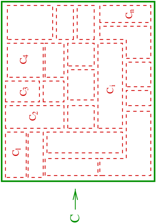
Figure 1: Subdivison of a large loop $C$ into smaller regions bounded by loops $\{C_{i}\}$. Note that the sum of interior perimeters may be much greater than the total perimeter of $C$.

Let us consider a very large planar loop $C$ whose minimal area ${\cal A}(C)$ is subdivided into some number $n$ of subareas ${\cal A}(C_{i})$, encircled by loops $C_{i}$ (Fig. 1). If all loops $C_{i}$ are large, and the coupling is strong, the question is to what extent the holonomies $U(C_{i})$ fluctuate independently. Let $F[g]$ denote any class function with character expansion

$$F[g]=\sum_{j\neq 0}f_{j}\chi_{j}(g)$$ (15)

The test for whether the $U(C_{i})$ fluctuate independently is whether or not the VEV of the product of $F[U(C_{i})]$ equals the product of the VEVs, i.e.

$$<\prod_{i}F[U(C_{i})]>\stackrel{{\scriptstyle?}}{{=}}\prod_{i}<F[U(C_{i})]>$$ (16)

In D=2 dimensions, it is easy to verify that the equality holds

$$<\prod_{i=1}^{n}F[U(C_{i})]> \approx \left(\prod_{i}2f_{1/2}\right)\exp\left[-\sigma_{1/2}{\cal A}(C)\right]$$ (17)

$$= \prod_{i=1}^{n}<F[U(C_{i})]>$$

so the group elements $U(C_{i})$ do seem to fluctuate independently in each subregion.

In $D>2$ dimensions the answer is different. Suppose that each $C_{i}$ satisfies
${\cal A}(C_{i})\gg 2{\cal P}(C_{i})$ in lattice units. In that case, we find from the strong-coupling expansion the leading contribution to the VEV of products

$$<\prod_{i=1}^{n}F[U(C_{i})]> \approx \left({1\over 3}\right)^{n-1}f_{1}^{n}<\chi_{1}[U(C)]>$$ (18)

$$= \left({1\over 3}\right)^{n-1}f_{1}^{n}\exp[-\mu{\cal P}(C)]$$

where $\mu=4\sigma_{1/2}$. The powers of $1/3$ are due to the fact that this contribution is highly non-planar, and would vanish in the large-N limit. The planar contribution, however, has an area law falloff, and for any finite N it is negligible for large loops. Likewise, for the product of VEVs, we have the leading contribution

$$\prod_{i=1}^{n}<F[U(C_{i})]> \approx \prod_{i}f_{1}<\chi_{1}[U(C_{i})]>$$ (19)

$$= f_{1}^{n}\exp\left[-\mu\sum_{i}{\cal P}(C_{i})\right]$$

However, for $n\gg 1$,

$$\sum_{i=1}^{n}{\cal P}(C_{i})\gg{\cal P}(C)$$ (20)

from which we see that the exponential falloff of $<\prod_{i}F[U(C_{i})]>$ and $\prod_{i}<F[U(C_{i})]>$ is quite different, already at the leading terms in the exponents. The conclusion is that the group elements $U(C_{i})$ do not, in fact, fluctuate independently; the deviations from pure random in the set of sub-loop probability distributions must be correlated.

On the other hand, since the area-law falloff of Wilson loops is supposed to be due to magnetic disorder; some component of magnetic flux should be fluctuating (nearly) independently. It is easy to check, at strong coupling, that the center elements ${\cal Z}[U(C_{i})]$ have the required property. The leading behavior for the VEV of the product is given by

$$<\prod_{i}{\cal Z}[U(C_{i})> = <\prod_{i}\mbox{signTr}[U(C_{i})]>$$ (21)

$$\approx <\prod_{i}\left(3\over 8\pi\right)\chi_{1/2}[U(C_{n})]>$$

$$\approx \exp[-\sigma_{1/2}{\cal A}(C)]\left(3\over 4\pi\right)^{n}$$

Similarly, for the product of the VEVs

$$\prod_{i}<{\cal Z}[U(C_{i})> = \prod_{i}<\mbox{signTr}[U(C_{i})]>$$ (22)

$$\approx \prod_{i=1}^{n}\left(3\over 4\pi\right)\exp[-\sigma_{1/2}{\cal A}(C_{i})]$$

Comparing (21) and (22), we see that

$$<\prod_{i}{\cal Z}[U(C_{i})]>\approx\prod_{i}<{\cal Z}[U(C_{i})]>$$ (23)

The center elements of the holonomies therefore fluctuate independently.

Any SU(2) class function $F[U(C_{i})]$ can be expressed as a function of of the sign and the modulus of Tr$[U(C_{i})]$ as follows:

$$F[U(C_{i})]=F_{1}[\mbox{Tr}^{2}\{U(C_{i})\}]+{\cal Z}[U(C_{i})]F_{2}[\mbox{Tr}^{2}\{U(C_{i})\}]$$ (24)

VEVs of products of $F_{1}$ and $F_{2}$ do not factorize, as seen in eqs. (18-20), while products of the ${\cal Z}[U(C_{i})]$ do factorize, as seen above in (23). The conclusion is that there is magnetic disorder in the center elements ${\cal Z}$ of the SU(2) group holonomies, but not in the coset elements, which depend only on $\mbox{Tr}^{2}[U(C)]$.

All of this has some bearing on the question of what are the relevant confining configurations in non-abelian gauge theory. Confining configurations, whatever they may be in D=3 and D=4 dimensions, must have the property of disordering the signs of Wilson loops, but not disordering the absolute values of those loops. At least, we have seen that this must be true at strong coupling. A class of configurations with these properties is the “spaghetti vacuum” of center vortices, proposed twenty years ago, in various forms, by ’t Hooft [1], Mack [2], the Copenhagen group [3, 4, 5, 6], and others [7, 8, 9]. A center vortex, linking loop $C$, has the property of sending $U(C)\rightarrow zU(C)$; such configurations can only disorder the center elements (i.e. the signs of Wilson loops, in SU(2)), leaving the rest of the group distribution untouched. This seems to be exactly what is needed.

On the other hand, it is not at all excluded that there could be some other degrees of freedom associated with loops that also fluctuate independently, and contribute to magnetic disorder. In our discussion so far we have only considered the holonomies $U(C)$, but we could also imagine using, e.g., an adjoint Higgs field (either elementary or composite) to construct other types of loop elements that might fluctuate independently. In fact, this is the general idea behind monopole confinement: An adjoint Higgs field is used to single out a U(1) subgroup of SU(2), and it is U(1) group elements, associated with loops $C_{i}$, that are disordered via a monopole condensate. From this point of view, the $Z_{2}$ disorder could be just a subset of a more general U(1) disorder. The simplest and most explicit proposal for monopole confinement (and U(1) disorder) in a non-abelian gauge theory is due to Polyakov, in his analysis of the D=3 Georgi-Glashow model [15, 16]. Since $GG_{3}$ interpolates smoothly between $QED_{3}$ and pure $YM_{3}$, we would now like consider if there is any remnant of $Z_{2}$ disorder in the 3D Georgi-Glashow model.

3 Double-Charged Loops in $\mathbf{GG_{3}}$

The full lattice action of the Georgi-Glashow model is a function of the gauge field variables $U_{\mu}(x)$ and the adjoint Higgs field variables $\phi(x)$

$$S[U,\phi] = \frac{1}{2}\beta_{G}\sum_{plaq}\mbox{Tr}[UUU^{\dagger}U^{\dagger}]$$ (25)

$$+ \frac{1}{2}\beta_{H}\sum_{x,\mu}\mbox{Tr}[U_{\mu}(x)\phi(x)U_{\mu}^{\dagger}(x)\phi^{\dagger}(x+\hat{\mu})]$$

$$- \sum_{x}\left\{\frac{1}{2}\mbox{Tr}[\phi\phi^{\dagger}]+\beta_{R}\left(\frac{1}{2}\mbox{Tr}[\phi\phi^{\dagger}]-1\right)^{2}\right\}$$

where

$$\phi(x)=\sum_{a=1}^{3}\phi^{a}(x)\sigma_{a}$$ (26)

The naive continuum limit is obtained from the lattice action by the following scaling:

$$U_{\mu}(x)=e^{iaA_{\mu}(x)},~{}~{}(A_{\mu}\equiv\frac{1}{2}\sigma^{a}A_{\mu}^{a}),~{}~{}~{}~{}~{}~{}\phi=a^{1/2}\beta^{1/2}_{R}\varphi,$$ (27)

and the identification of continuum couplings $g$, $\lambda$ and $\mu$ by

$$\beta_{G}=\frac{4}{g^{2}a},~{}~{}~{}\frac{\beta_{R}}{\beta_{H}}=\frac{1}{4}\lambda\,a,~{}~{}~{}\frac{1-3\beta_{H}-2\beta_{R}}{\beta_{H}}=-\frac{1}{2}\mu\,a^{2}.$$ (28)

Thus the continuum action becomes

$$S_{cont}=-\int d^{3}x\;\frac{1}{2}{\rm Tr}\,\Bigl{[}\frac{1}{g^{2}}\,F_{\mu\nu}^{2}+\frac{1}{2}\Bigl{(}D_{\mu}\varphi\Bigl{)}^{2}-\frac{1}{2}\mu\,\varphi^{2}+\frac{1}{4}\lambda\,\varphi^{4}\Bigr{]},$$ (29)

where $D_{\mu}\varphi=\partial_{\mu}\varphi+i[A_{\mu},\varphi]$. It is obtained for

$$\beta_{G}\to\infty,~{}~{}~{}\beta_{R}\to 0,~{}~{}~{}\beta_{H}\to\frac{1}{3},$$ (30)

the approach monitored by the lattice spacing $a$. A more precise description is obtained by taking into account that although the coupling constants are not renormalized in three dimensions, the masses $M_{W}$ and $M_{\varphi}$ are renormalized. We refer to [18] for formulas which include the one-loop mass renormalizations. The tree-formulas describe correctly the qualitative features which have our interest. In the “broken” region, where the approach of $\beta_{H}$ to 1/3 is from above, it corresponds mass $M_{W}$ for the charged vector particle and a mass $M_{\varphi}$ for the neutral scalar, given by:

$$M^{2}_{W}=g^{2}\,\varphi_{c}^{2},~{}~{}~{}M_{\varphi}^{2}=2\mu\,\varphi^{2}_{c},~{}~{}~{}~{}\varphi_{c}^{2}=\frac{\mu}{\lambda}.$$ (31)

If we in the limit (30) increase $\beta_{H}$ away from 1/3, it corresponds formally to a “continuum” limit where

$$M_{W}\sim\frac{1}{a},~{}~{}~{}~{}M_{\varphi}\sim\frac{1}{a},$$ (32)

i.e. a limit where only the free photon field is present as a physical excitation. More generally, taking $\beta_{G}$ and $\beta_{R}$ fixed and $\beta_{H}\to\infty$ have the same effect, except that the resulting effective theory will be compact lattice $U(1)$, where we obtain the continuum free photon field only in the limit $\beta_{G}\to\infty$. For future reference let us note that the tree-value formulas (28) and (31) lead to the following expressions for dimensionless ratio

$$\frac{M_{W}}{g^{2}}=\frac{\beta_{H}\beta_{G}}{4}\left(\frac{3-(1-2\beta_{R})/\beta_{H}}{2\beta_{R}}\right)^{\frac{1}{2}}.$$ (33)

The actual region above $\beta_{H}=1/3$ where $M_{W}$ is not of the order of the inverse lattice spacing $a$ is very narrow, in agreement with numerical simulations [18].

Going to the unitary gauge, we write

$$S_{ug}[U,\rho]\equiv S[U,\phi(x)=\rho(x)\sigma_{3}]$$ (34)

The unitary gauge action $S_{ug}$ still has a residual $U(1)$ gauge symmetry. We may factor the SU(2) link variable into a matrix $A_{\mu}$ which transforms under the residual symmetry like a $U(1)$ gauge field, and a piece $C_{\mu}$ transforming like a double-charged matter field [19]

$$U_{\mu}(x) = \left(\begin{array}[]{cc}\cos\varphi e^{i\theta}&\sin\varphi e^{i\chi}\cr-\sin\varphi e^{-i\chi}&\cos\varphi e^{-i\theta}\end{array}\right)$$ (37)

$$= \left(\begin{array}[]{cc}\cos\varphi&\sin\varphi e^{i\gamma}\cr-\sin\varphi e^{-i\gamma}&\cos\varphi\end{array}\right)\left(\begin{array}[]{cc}e^{i\theta}&0\cr 0&e^{-i\theta}\end{array}\right)$$ (42)

$$= \left(\begin{array}[]{cc}\sqrt{1-cc^{*}}&c\cr-c^{*}&\sqrt{1-cc^{*}}\end{array}\right)\left(\begin{array}[]{cc}e^{i\theta}&0\cr 0&e^{-i\theta}\end{array}\right)=C_{\mu}(x)A_{\mu}(x)$$ (47)

with lattice measure

$$\int dU={1\over 2\pi^{2}}\int_{0}^{\pi/2}d\varphi~{}\cos\varphi\sin\varphi\int^{\pi}_{-\pi}d\theta\int^{\pi}_{-\pi}d\chi$$ (48)

The effective abelian action $S_{eff}[A]$ for $GG_{3}$ is then defined by

$$e^{S_{eff}[A]}\equiv\int\prod_{x}d\rho(x)\prod_{\mu}d\varphi_{\mu}(x)d\chi_{\mu}(x)\cos\varphi_{\mu}(x)\sin\varphi_{\mu}(x)~{}e^{S_{ug}[U,\rho]}$$ (49)

The question we wish to raise is whether the Euclidean quantum theory of $S_{eff}[A]$, at large scales, is correctly represented by a monopole Coulomb gas, as proposed in [15], since this is the generic model of monopole confinement. In particular, consider the “abelian” Wilson loops

$$A_{n}(C)=\mbox{Tr}[(AAA...A)^{n}]$$ (50)

corresponding to closed loops of heavy particles carrying $n$ units of the abelian electric charge, with

$$<A_{n}(C)>={1\over Z}\int DA~{}A_{n}(C)e^{S_{eff}[A]}$$ (51)

The crucial point is that in $GG_{3}$, the string-tension $\sigma_{n}$ of loops $<A_{n}(C)>$ should vanish asymptotically, if $n$ is an even integer. The reason is simply that the Georgi-Glashow model contains massive W-bosons which carry two units of electric charge; these correspond to the $C_{\mu}(x)$ degrees of freedom. The W-bosons are able to screen static sources carrying an even number of unit electric charges. If a flux tube were to form between $n$=even charged sources, with some string tension $\sigma_{n}=T$ then at a separation of roughly

$$L={nM_{W}\over T}$$ (52)

charge-screening by W-bosons becomes energetically favorable and the flux-tube breaks, so $\sigma_{n}=0$ asymptotically. Although $S_{eff}[A]$ contains only the abelian gauge field, it must somehow incorporate this non-confinement of even charges, since we can always rewrite eq. (51) as

$$<A_{n}(C)>=\int DAD\varphi D\chi D\rho~{}A_{n}(C)e^{S_{ug}[C_{\mu}A_{\mu},\rho]}$$ (53)

where the charged fields are included explicitly.

3.1 Strong coupling expansion

While charge-screening may be expected in $GG_{3}$ on very general grounds, it is also possible to verify the effect explicitly in a strong-coupling expansion. Take, for simplicity, $\beta_{R}=\infty$ so that the modulus of the Higgs field is “frozen” to $\rho=1$, with $\beta_{H}$ chosen large enough such that $M_{W}\gg 1$ in lattice units, and $\beta_{G}$ small enough to allow a strong-coupling expansion. Expanding the action to 2nd order in $c,~{}c^{*}$, one easily finds for large, double-charged loops the perimeter falloff expression

$$<A_{2}(C)>=\exp[-\mu{\cal P}(C)]~{}~{}~{}~{}~{}~{}(\mbox{GG}_{3})$$ (54)

with perimeter coefficient, extracted from the leading diagram,

$$\mu=-\log\left[{\beta_{G}^{2}\over 8\beta_{H}}{1-2\beta_{H}e^{-2\beta_{H}}-e^{-2\beta_{H}}\over 1-e^{-2\beta_{H}}}\right]$$ (55)

In strong-coupling compact QED, of course, the answer is different. There are no charged bosons to screen the double-charged loop, and its value, for the Wilson action, is

$$<A_{2}(C)>=\exp[-2\sigma{\cal A}(C)]~{}~{}~{}~{}~{}~{}(QED_{3})$$ (56)

with $\sigma$ the string tension of the single-charged loop. For multiply charged loops $<A_{n}(C)>$ in strongly-coupled compact $QED_{3}$, the string tension is in general $n$ times the string tension for single-charged loops. Thus we have a qualitative difference, at least in strong-coupling, between compact $QED_{3}$ and $S_{eff}[A]$ of the 3D Georgi-Glashow model, because in the latter effective abelian theory, there is no string tension for $<A_{n}(C)>$ when $n$ is even.

For compact $QED_{3}$, it is possible to derive the result (56) also at weak couplings, which we do in the next section. This is an interesting result in its own right, since the existence of the $n=2$ string tension in compact $QED_{3}$ has been questioned (ref. [16], p. 80), while, in numerical simulations, a finite value equal to twice the $n=1$ value has been measured [20].

3.2 Double-Charged Loops in a Monopole Gas

It is well known that compact $U(1)$ on a lattice can be written in a monopole gas represention. If we use the Villain version of compact $U(1)$ one obtains [21]

$$Z_{mon}=\sum_{m(r)=-\infty}^{\infty}\exp\Bigl{[}-\frac{2\pi^{2}}{g^{2}a}\sum_{r,r^{\prime}}m(r^{\prime})G(r-r^{\prime})m(r)\Bigr{]},$$ (57)

where $m(r)$ is an integer valued monopole field at the (dual) lattice size $r$, $G(r-r^{\prime})$ is the lattice Coulomb propagator in three dimensions, i.e. $\Delta_{\mu}^{2}G(r-r^{\prime})=-\delta_{rr^{\prime}}$, and $g^{2}a$, $a$ being the lattice spacing, is the temperature $1/\beta$ in the usual thermodynamic interpretation.

One can represent the propagator $G(r-r^{\prime})$ by a Gaussian functional integral:

$$Z_{mon} = \int\prod_{r}d\chi(r)\;\exp\Bigl{[}-\frac{g^{2}a}{4\pi^{2}}\sum_{r}\frac{1}{2}(\Delta_{\mu}\chi(r))^{2}\Bigr{]}$$ (58)

$$\times\sum_{m(r)=-\infty}^{\infty}\exp\Bigl{[}-{2\pi^{2}\over g^{2}a}G(0)\sum_{r}m^{2}(r)+i\sum_{r}m(r)\chi(r)\Bigr{]}.$$

In the weak coupling limit (low temperature limit) where $g^{2}a\to 0$ we need only to maintain the first terms $|m(r)|\leq 1$ in the sum and we get

$$Z_{mon}\approx\int\prod d\chi(r)\;\exp\Bigl{[}-\frac{g^{2}a}{4\pi^{2}}\sum_{r}\Bigl{(}\frac{1}{2}(\Delta_{\mu}\chi)^{2}+M_{0}^{2}(1-\cos\chi(r))\Bigr{)}\Bigr{]},$$ (59)

where $M^{2}_{0}$ comes from the propagator $G(r-r^{\prime})$ for coinciding arguments, ($G(0)\approx 0.253$ [22])

$$M^{2}_{0}=\frac{8\pi^{2}}{g^{2}a}\,\exp\Bigl{[}-\frac{2\pi^{2}}{g^{2}a}\,G(0)\Bigr{]}.$$ (60)

and if we interpret the monopoles as instantons, $2\pi^{2}G(0)/g^{2}a$ can be viewed as the action of the instanton.

Let us for notational simplicity carry out the following discussion in a continuum notation. All manipulations done in the following have a precise lattice analogy (see [21]). The translation is

$$\Delta_{\mu}\to a\,\partial_{\mu},~{}~{}~{}a^{3}\sum_{r}\to\int d^{3}r,$$ (61)

and we end up with

$$Z_{mon}\approx\int{\cal D}\chi(r)\;\exp\Big{[}-\frac{g^{2}}{4\pi^{2}}\int d^{3}r\;\Bigl{(}\frac{1}{2}(\partial_{\mu}\chi)^{2}+M^{2}(1-\cos\chi(r))\Bigr{)}\Bigr{]}.$$ (62)

where

$$M^{2}=a^{-2}M_{0}^{2}.$$ (63)

In the Coulomb gas approximation we are effectively integrating over the electromagnetic fields carried by the monopoles. They can be found from the monopole density $m(r)$ by integrating

$$\partial_{\mu}H_{\mu}(r)=2\pi\,m(r),~{}~{}~{}{\rm i.e.}~{}~{}~{}H_{\mu}(r)=\frac{1}{2}\int d^{3}r^{\prime}\;\frac{(r-r^{\prime})_{\mu}}{|r-r^{\prime}|^{3}}\;m(r^{\prime}),$$ (64)

In particular we find, if $C$ denotes a closed curve and $S(C)$ a surface with $C$ as boundary, that

$$\oint_{C}dr_{\mu}A_{\mu}(r)=\int_{S(C)}dS_{\mu}(r)\;H_{\mu}(r)=\int d^{3}r\;\eta_{S(C)}(r)\;m(r),$$ (65)

where

$$\eta_{S(C)}(r)=-\frac{1}{2}\frac{\partial}{\partial r_{\mu}}\int_{S(C)}dS_{\mu}(r^{\prime})\;\frac{1}{|r-r^{\prime}|}.$$ (66)

It is seen that $\eta(r)$ has the interpretation as a dipole sheet on the surface $S(C)$. Thus, if $C$ is a planar curve in the $(x,y)$ plane and $S(C)$ the planar surface with $C$ as boundary curve, we have

$$-\partial^{2}\eta_{S(C)}=2\pi\delta^{\prime}(z)\theta_{S}(x,y),$$ (67)

where $\theta_{S(C)}(x,y)$ is one for a point inside the boundary $C$ and zero for a point outside the boundary $C$. Close to the surface $S$ we have

$$\eta(r)=\pi{\rm sign}\,z\;\theta_{S}(x,y),$$ (68)

i.e. it jumps by $2\pi$ when passing the dipole sheet.

We can now calculate the expectation value of a planar Wilson loop which carries n units of charge. From (65) we obtain

$$\langle A_{n}(C)\rangle\equiv\langle e^{in\oint dr_{\mu}\;A_{\mu}(r)}\rangle=\langle e^{in\int d^{3}r\;\eta_{S(C)}(r)\;m(r)}\rangle,$$ (69)

where the expectation value is calculated with respect to the partition function (57). Performing the same transformations which lead from (57) to (62), the last term in (69) leads to a translation of $\chi(r)$ such that one obtains

$$\langle A_{n}(C)\rangle=\frac{1}{Z_{mon}}\int{\cal D}\chi(r)\;\exp\Bigl{[}-\frac{g^{2}}{4\pi}\int d^{3}r\;\Bigl{(}\frac{1}{2}(\partial_{\mu}(\chi-n\eta_{S(C)})^{2}+M^{2}(1-\cos\chi(r))\Bigr{)}\Bigr{]},$$ (70)

Since we consider the weak coupling regime the dominant contribution to the expectation value (70) comes from the classical solution to the effective action in (70). In case we choose the planar loop to lie in the $(x,y)$ plane we obtain from (67):

$$\partial^{2}\chi=2\pi n\delta^{\prime}(z)\theta_{S}(x,y)+M^{2}\sin\chi.$$ (71)

A solution to the homogeneous equation is (far from the boundary, suppressing a trivial $(x,y)$ dependence):

$$\chi^{(0)}(z)=4\arctan e^{-Mz}.$$ (72)

Note that for $z<0$ it can be written as $-4\arctan e^{Mz}+2\pi$. Thus, for $n=1$, eq. (71) has, far away from the boundary $C$, the solution

$$\chi_{cla}^{(1)}={\rm sign}\,z\cdot 4\arctan(e^{-M\,|z|})\,\theta_{S}(x,y).$$ (73)

The important property of the solution (73) is that $\chi_{cla}^{(1)}(z)\to 0$ for $|z|\to\infty$. This implies that it can be joined to the trivial solution $\chi=0$ for $|r|\to\infty$ in $R^{3}$.

Since the solution $\chi_{cla}^{(1)}$ is given in terms of elementary functions one can calculate the corresponding action in (70):

$$\int d^{3}x\Bigl{(}\frac{1}{2}(\partial_{\mu}(\chi_{cla}^{(1)}-\eta_{S(C)})^{2}+M^{2}(1-\cos\chi^{(1)}_{cla}(x))\Bigr{)}=8M\,{\rm Area}(S)+{\rm perimeter~{}contributions}.$$ (74)

In this way one obtains the famous area law of Wilson loops [15] in the three dimensional Coulomb gas of monopoles since it follows from (70) that

$$\langle A_{1}(C)\rangle\approx\exp\Bigl{[}-\frac{g^{2}}{4\pi^{2}}\,8M\;{\rm area}(S)\Bigr{]}.$$ (75)

Let us now consider the situation for double charged Wilson loops. In order to find the minimum of the action we should solve (71) for $n=2$. One could be misled to suggest the simple solution (far from the boundary of $C$)

$$\chi_{cla}^{(2)}(z)=2\pi{\rm sign}\,z,~{}~{}~{}{\rm i.e.}~{}~{}~{}\chi(z)=2\eta(z).$$ (76)

This clearly gives energy zero in the interior of the Wilson loop and seemingly no area law (as for the full Georgi-Glashow model). However, since this solution does not go to zero far from the Wilson loop, contrary to the solution (73) for $n=1$, we have to interpolate between the limiting values $\chi_{cla}^{(2)}(z)=2\pi$ and $\chi_{cla}^{(2)}(z)=-2\pi$ in some region in space far away from the Wilson loop. This will cost an energy which is easily seen to be proportional to the area of the “domain wall” where the interpolation takes place. Thus the optimal situation is also here one where $\chi_{cla}^{(2)}(z)\to 0$ for $|z|\to\infty$. With this requirement it follows that we have to solve eq. (71) with the boundary conditions that $\chi_{cla}^{(2)}(z)\to 0$ for $|z|\to\infty$ and $\chi_{cla}^{(2)}(z)-2\eta(z)$ is differentiable for $z=0$ when passing the sheet.

There is no such solution. But we can find approximate solutions with energies above, but arbitrary close to twice the energy corresponding $\chi_{cla}^{(1)}$. From (71), (73) and (72) it follows that for $z_{0}\gg 1/M$

$$\chi^{(2)}(z)=\theta(z)\,\chi^{(0)}(z-z_{0})+\theta(-z)(\chi^{(0)}(z+z_{0})-2\pi)$$ (77)

is a solution to (71) with $n=2$ except for exponentially small corrections, and its energy is twice that of $\chi^{(1)}_{cla}$ except for exponentially small corrections. Further we see that this approximate solution behaves like (76) for $|z|<<z_{0}$.

It is interesting that one can find a different kind of solution with the same features, namely that the energy of the classical solution can be arbitrary close to twice that of $\chi_{cla}^{(1)}$, but never reach it. We have a free choice for the surface $S(C)$, except for the requirement that $C$ is the boundary of $S$. In particular, we could for the doubled charged Wilson loop choose two sheets separated a distance $2d$ and located in the $z=\pm d$-planes, except close to the boundary $C$. For each sheet we now have a discontinuity corresponding to $\eta(z)$. If $d>>1/M$ it is clear that the solution, except for exponentially small corrrections, has to be

$$\chi^{(2)}(z)=\theta(-z)\chi^{(1)}_{cla}(z+d)+\theta(z)\chi^{(1)}_{cla}(z-d)W.$$ (78)

The energy becomes minimal (and equal two times that corresponding to $\chi^{(1)}_{cla}(z)$) in the limit $d\to\infty$.

We conclude that the string tension for a double-charged Wilson loop will be twice the string tension of a single charged Wilson loop if we restrict ourselves to the Coulomb gas approximaton of functional integral. Clearly the arguments can be extended to $n$-charged Wilson loops.

3.3 Weak coupling limit of lattice $\mathbf{GG_{3}}$

The monopole gas calculation above was a weak coupling expansion in the sense that $g^{2}a$ had to be considered small in order to make the truncation (59). In particular this implied that the monopole “action” $2\pi^{2}G(0)/g^{2}a$ is large and the density of monopoles,

$$\rho\sim\exp\Bigl{(}-\frac{2\pi^{2}G(0)}{g^{2}a}\Bigr{)},$$ (79)

exponentially small. In the naive continuum limit, as defined by (28)-(31), we can make contact to the similar instanton calculations in the continuum $GG_{3}$ model. In that case the instanton (monopole) action is given by

$$S_{mon}=\frac{M_{W}}{g^{2}}\,\epsilon(\lambda/g^{2}),$$ (80)

where $\epsilon(x)$ is a slowly varying function of $x$ ($\epsilon(0)=4\pi$). (It is seen that one obtains the $QED_{3}$ formulas in the limit where $M_{W}\sim 1/a$, as expected). A dilute instanton calculation is valid if the density of instantons,

$$\rho\sim\exp(-S_{mon}),$$ (81)

is exponentially small relatively to the extension of the instantons (which is $\approx 1/M_{W}$). Thus the calculation in the last subsection is valid in $GG_{3}$ provided $M_{W}/g^{2}\gg 1$. One obtains a string tension for an $n$-charged Wilson loop

$$T_{n}\sim n\;e^{-S_{mon}}\,\times\,[\mbox{subleading corrections}].$$ (82)

To the extent one can trust the tree-value formulas, the lattice inequality corresponding to $M_{W}/g^{2}\gg 1$ can be obtained from (33):

$$\frac{M_{W}}{g^{2}}\sim\frac{\beta_{H}\beta_{G}}{4}\left(\frac{3-(1-2\beta_{R})/\beta_{H}}{2\beta_{R}}\right)^{\frac{1}{2}}\gg 1.$$ (83)

This formula is most reliable for $\beta_{G}$ large (and $\beta_{R}$ is small) and $\beta_{H}$ close to $(1-2\beta_{R})/3$.

We have seen above (see eq. (52)) that we expect a perimeter law in $GG_{3}$ for $n$-charged Wilson loops, $n$ even, provided the linear extension $L$ of the loop satisfies

$$L>\frac{nM_{W}}{T_{n}}\sim e^{S_{mon}}\times[\mbox{subleading corrections}]$$ (84)

This length is much larger than the length scale

$$\xi_{\sigma}=\sigma^{-1/2}\sim\exp\Bigl{(}\frac{1}{2}S_{mon}\Bigr{)},$$ (85)

set by the string tension, and it is also much greater than the average distance

$$R=\rho^{-1/3}\sim\exp\Bigl{(}\frac{1}{3}S_{mon}\Bigr{)},$$ (86)

between the monopoles. Typically we will have to go to distances larger than $\xi_{\sigma}$ if we want to measure the string tension. However, for $M_{W}/g^{2}\gg 1$ we have to move out exponentially many units of length $\xi_{\sigma}$ before an $n$-charged string, $n$ even, breaks:

$$\frac{L}{\xi_{\sigma}}\sim\exp\Bigl{(}\frac{1}{2}S_{mon}\Bigr{)}\times[\mbox{subleading corrections}].$$ (87)

In the lattice $GG_{3}$ model (25) the parameter $\beta_{H}$ allows us to interpolate continuously between compact $QED_{3}$ (large $\beta_{H}$) and pure Yangs-Mills theory ($\beta_{H}\to 0$). From the tree-formula (83) we see (for large $\beta_{G}$) how large $\beta_{H}$ corresponds to a value $M_{W}/g^{2}\gg 1$, while $M_{W}/g^{2}$ drops to zero (in the tree-approximation) for $\beta_{H}=(1-2\beta_{R})/3$. Below this value of $\beta_{H}$ we have the “unbroken” coupling region of the Yang-Mills-Higgs system, where we expect the center $Z_{2}$ to play the dominant role in confinement and the monopole gas description is not valid at all.

4 $\mathbf{Z_{2}}$ Disorder in $\mathbf{GG_{3}}$

We now return to the question of $Z_{2}$ disorder in $GG_{3}$. Considering only the abelian magnetic flux probed by loops $A_{n}(C)$, we can ask if disorder is distributed evenly in the $U(1)$ group, or if it is only present in some subset of the degrees of freedom. Our procedure is the same as in section 3. Defining again the holonomy distributions on the compact $U(1)$ group

$$P_{C}(e^{i\omega}) = <\delta[\omega,\theta(C)]>=<\sum_{n=-\infty}^{\infty}e^{in[\omega-\theta(C)]}>$$

$$\tilde{P}_{C}(e^{i\omega}) = P_{C}(e^{i\omega})-1$$ (88)

we see that for compact $QED_{3}$ the approach to a pure random distribution has an area-law falloff

$$\tilde{P}_{C}(e^{i\omega})\sim\cos(\omega)e^{-\sigma{\cal A}(C)}~{}~{}~{}~{}~{}(QED_{3})$$ (89)

while in $GG_{3}$, the approach goes, asymptotically, as a perimeter-law falloff

$$\tilde{P}_{C}(e^{i\omega})\sim\cos(2\omega)e^{-\mu{\cal P}(C)}~{}~{}~{}~{}~{}~{}(GG_{3})$$ (90)

due to the different behavior of the $n=$even charged loops. However, once again, there is a hidden area-law approach to randomness also in $GG_{3}$, since if we define

$${\cal Z}[A(C)]=\mbox{sign}\cos[\theta(C)]$$ (91)

and the probabilities

$$P_{C}(z)=<\frac{1}{2}(1+z\times\mbox{sign}[\cos\theta(C)])>$$ (92)

with $z=\pm 1$ and $\tilde{P}_{C}(z)=P_{C}(z)-\frac{1}{2}$, then in $GG_{3}$

$$\tilde{P}_{C}(z)\sim ze^{-\sigma{\cal A}(C)}$$ (93)

Turning to lattice strong coupling we again find, in complete analogy to the pure-gauge theory in section 3, that at leading order for compact $QED_{3}$

$$<\prod_{i}F[A(C_{i})]>\approx\prod_{i}<F[A(C_{i})]>~{}~{}~{}~{}~{}(QED_{3})$$ (94)

while in $GG_{3}$

$$<\prod_{i}F[A(C_{i})]> \sim e^{-\mu{\cal P}(C)}$$

$$\prod_{i}<F[A(C_{i})]> \sim e^{-\mu\sum_{i}{\cal P}(C_{i})}$$ (95)

It follows that, in contrast to $QED_{3}$, the abelian loop elements do not fluctuate independently in $GG_{3}$, even at very strong lattice coupling. On the other hand, the $Z_{2}$ elements

$$<\prod_{i}{\cal Z}[A(C_{i})]> = \prod_{i}e^{-\sum_{i}{\cal A}(C_{i})}$$ (96)

$$= \prod_{i}<{\cal Z}[A(C_{i})]>$$

do fluctuate independently in $GG_{3}$, at strong coupling.

The conclusion is that even in $GG_{3}$, long-range disorder seems to be associated with a $Z_{2}$, rather than a $U(1)$, subgroup; there is again disorder in the sign, but not in the modulus, of loop elements $\cos\theta(C)$. The inclusion of an adjoint Higgs field does not seem to change the fact that disorder, at large scales, is essentially a property of the gauge group center. In the last section we gave a qualitative description of the length scales in $GG_{3}$ beyond which the Coulomb gas picture breaks down and where (as we have now argued) the magnetic disorder is center disorder.

4.1 Extension to SU(N)

All of the arguments above are readily extended to theories with an SU(N) gauge group; we will only indicate briefly how this goes. The probability distribution $P_{C}(g)$ in eq. (1) generalizes in the obvious way, with the sum over $j$ replaced by a sum over $SU(N)$ representations. Writing

$$\chi_{F}(g)=Ae^{i\phi}$$ (97)

where $F$ denotes the fundamental representation, $A\geq 0$ is real, and $\phi\in[0,2\pi)$, let

$$n(g) = \mbox{int}\left[{N\phi\over 2\pi}\right]$$

$${\cal Z}(g) = \exp[2\pi in(g)/N]$$ (98)

where int($x$) denotes the integer part of the real number $x$. This definition assigns a center element to every group element, with the property that ${\cal Z}(zg)=z{\cal Z}(g)$ for $z\in Z_{N}$. Then

$$P_{C}(z)=<\Phi[z,U(C)]>~{}~{}~{}\mbox{where}~{}~{}~{}\Phi[z,U(C)]=\left\{\begin{array}[]{cl}1&\mbox{if~{}}z={\cal Z}[U(C)]\cr 0&\mbox{otherwise}\end{array}\right.$$ (99)

gives the probability that ${\cal Z}[U(C)]=z$.

Arguments entirely analogous to those in sections 2 and 3 show that the holonomy probability $P_{C}(g)$ approaches the random distribution with only a perimeter-law falloff, while $P_{C}(z)$ approaches the random distribution with an area-law falloff. At strong-couplings, the center elements ${\cal Z}[U(C_{i})]$ fluctuate independently in sub-areas of a large loop, while class functions $F[U(C_{i})]$ in general do not. From this we conclude that there is magnetic disorder among the center elements, but not in the coset. Once again, it should be noted that the correlation among $SU(N)/Z_{N}$ coset elements relies on non-planar contributions, which are dominant for large loops. If we would take the large-N limit before the large-loop limit, then there is Casimir scaling as in D=2 dimensions, and disorder throughout the group manifold.

Introducing an adjoint Higgs field in $D=3$ dimensions, and fixing to unitary gauge, we can define the loop observables (in continuum notation), invariant under the remnant $U(1)^{N-1}$ subgroup

$$<rk|A(C)|rk>=\left[\exp[i\oint_{C}dx^{\mu}~{}A_{\mu}^{i}(x)H^{r}_{i}]\right]_{kk}$$ (100)

where $H^{r}_{i}$ denotes the $i$-th generator of the Cartan subalgebra in representation $r$ of the SU(N) group, and $(kk)$ is just an element of the dim($r$)$\times$dim($r$) diagonal matrix $A(C)$ in this represention. The $Z_{N}$ center elements ${\cal Z}[A(C)]$ are extracted, as above, from the phase of $\chi_{F}[A(C)]$.

In the monopole Coulomb gas picture, disregarding the effects of the charged bosons, the string tension of $<rk|A(C)|rk>$ depends on both representation $r$ and choice of diagonal matrix element $(kk)$. Allowing, however, for the effects of the charged W-bosons, these string tensions can depend only on the N-ality of representation $r$, and are independent of $(kk)$. Asymptotically there is disorder in the ${\cal Z}[A(C)]$ elements, but not in the full $U(1)^{N-1}$ group manifold. The distribution of abelian magnetic flux, in the $Z_{N}$ disorder regime, is not that of a monopole Coulomb gas.

5 Discussion

We have stressed in this article the fact that, while massive virtual particles are often irrelevant to vacuum fluctuations in the far-infrared, this is not the case for massive charged particles in a confining theory. The screening of external charged sources by quanta of the matter field is, of course, a rather trivial point, and allows us to conclude that certain loop operators have a perimeter falloff. What may be slightly less obvious is the fact that such perimeter falloffs have implications for the probability distribution of large-scale vacuum fluctuations also in the absence of external charges. This point is best appreciated in, e.g., the 3D Georgi-Glashow model, by imagining an integration, in unitary gauge, over the W-bosons and Higgs field, to leave an effective action $S_{eff}[A]$ involving only the photon field. There are no longer any explicit, electrically charged fields left in the action to screen multiply-charged abelian loops. Instead, the effect of the virtual W-particles has gone into altering the Boltzman distribution for vacuum fluctuations of the abelian field, such that those abelian configurations which would lead to an area law for even-charged loops in the $Z_{2}$ regime have been suppressed. Thus the effective action $S_{eff}[A]$ is not only quantitatively but also qualitatively different, at large scales, from the $QED_{3}$ action with a lattice cutoff, and a monopole Coulomb gas picture is not adequate to describe the confining vacuum in the $Z_{2}$ regime.

The picture we are led to, for the onset of $Z_{2}$ disorder in the 3D Georgi-Glashow model, is indicated schematically in Fig. 2. For fixed $\beta_{G}$ and sufficiently large $\beta_{R}$, no phase transition is encountered as $\beta_{H}$ varies from $\beta_{H}=0$ ($YM_{3}$) to $\beta_{H}=\infty$ ($QED_{3}$) [18]. The curved solid line, however, represents the breaking of the adjoint string, and the loss of “Casimir scaling,” while the solid line tailing off in a dashed line represents the breaking of the flux tube between double-charged abelian sources. The dashed line indicates the complete breakdown of the Coulomb gas picture in unitary gauge, as $\beta_{H}\rightarrow 0$. All abelian Wilson loops vanish in this gauge in the $\beta_{H}=0$ limit, although it may still be possible to define the $n=2$ abelian charge screening distance by extrapolation from non-zero $\beta_{H}$. It would be interesting to know where the dashed line terminates.

Figure 2: Confining disorder, extracted from U(1) and SU(2) holonomies, in the 3D Georgi-Glashow model.

The absence of an adjoint string tension at any length scale, for sufficiently large $\beta_{H}$ at fixed ($\beta_{G},\beta_{R}$), has been seen in numerical simulations of $GG_{3}$ [14, 23], and is easily understood. A $j=1$ representation quark consists of two components ($m=\pm 1$) which are double-charged under the U(1) subgroup, and one component ($m=0$) which is neutral. When the confining field is essentially abelian, the neutral component is dominant, and the adjoint loop has no area-law falloff at any length scale. In fact, this gives us an interesting criterion for U(1) disorder in an SU(2) gauge theory, regardless of whether the adjoint scalar is elementary or composite. It is required that in the U(1) regime

1. Even-charged loops have area-law falloff. Otherwise, as we have seen, the loops are probing $Z_{2}$ disorder.

2. Adjoint loops have perimeter-law falloff. If not, then abelian neutral components are also subject to a confining force, and there is disorder over the entire group manifold; not only in a U(1) or $Z_{2}$ subgroup.

In D=4 dimensions, the maximal abelian gauge has been studied extensively in pure Yang-Mills theory. This gauge defines a composite adjoint Higgs field, U(1) holonomies, and monopole currents. The hope is that confining disorder is U(1) disorder which can be attributed, as in $GG_{3}$, to monopoles. Numerically, however, although double-charged loops defined in this formulation have an area-law falloff (cf. ref. [24]) at the length scales probed by Monte Carlo simulations, this is also true of the adjoint loops at the same distance scales; the second criterion above is not satisfied.

Returning to the 3D Georgi-Glashow model at large $\beta_{H}$, it is interesting to consider how the confining abelian fields are arranged at large scales, where there is $Z_{2}$ disorder. It is useful to think in terms of the effective abelian theory in (49), obtained from $GG_{3}$ in unitary gauge by integrating out the W and Higg fields. $S_{eff}[A]$ and $S[U,\phi]$ are of course equivalent, in unitary gauge, so far as the vacuum distribution of the A-field is concerned. $S_{eff}[A]$, like the $GG_{3}$ model from which it is obtained, will have instanton solutions corresponding to monopoles. However, since the monopole Coulomb gas picture breaks down at the onset of $Z_{2}$ disorder, it must be that the interactions among monopoles are not really Coulombic at long distances, and neither is the field distribution of the corresponding magnetic flux. This raises the interesting (although at this stage speculative) question of how the abelian flux from monopoles is actually organized, on distance scales characteristic of the $Z_{2}$ regime.

Figure 3: An example of monopole-antimonopole magnetic flux organized into $Z_{2}$ vortices.

As it is only the sign of $\cos\theta(C)$ which is disordered in the $Z_{2}$ regime, while the effective action $S_{eff}[A]$ only involves an abelian gauge field, there is a strong implication that the magnetic flux due to monopoles is collimated, at sufficiently large distance scales, in units of $\Phi_{B}=\pm\pi$. Collimated flux of these units, with a stochastic distribution of such “fluxons” across the minimal area of a large loop, affects only the sign of odd charged loops, leading to an identical string tension for all odd-charged loops, and yielding zero string tension for all even-charged loops. This is the proper result in the $Z_{2}$ disorder regime. If magnetic flux is, in fact, collimated in this way, then a $Z_{2}$ vortex picture in this regime is quite natural.

A particular example of $\pm 2\pi$ monopole flux organized into $Z_{2}$ vortex configurations of $\pm\pi$ flux is shown in Fig. 3. This is by no means the only possibility. In fact, at large $\beta_{H}$, the scale $L$ at which monopole flux should be collimated in units of $\pm\pi$ is actually much greater than the average monopole separation $R$, as seen by comparing eqs. (84) and (86). The illustration in Fig. 3 might be relevant at lower $\beta_{H}$, approaching the pure Yang-Mills limit, when $L/R$ is O(1). As $\beta_{H}\rightarrow\infty$, the width of the vortex regions would diverge to infinity, and the monopole Coulomb gas picture is valid at all distances. As $\beta_{H}$ is reduced, the vortex width decreases. A very attractive possibility is that abelian vortices in $GG_{3}$ smoothly transform into center vortices of the pure Yang-Mills theory as $\beta_{H}\rightarrow 0$, making contact with the ideas of refs. [1, 2, 3, 4, 5, 6, 7, 8, 9], and the numerics of refs. [10, 11, 12].

Acknowledgements

We have benefited from discussions with Alex Kovner and Poul Olesen.

J.A. acknowledges the support of the Professor Visitante Iberdrola Program and the hospitality at the University of Barcelona, where part of this work was done. J.G.’s research was supported in part by Carlsbergfondet, and in part by the U.S. Department of Energy under Grant No. DE-FG03-92ER40711.

References

- [1] G. ’t Hooft, Nucl. Phys. B138 (1978) 1.
- [2] G. Mack, in Recent Developments in Gauge Theories, edited by G. ’t Hooft et al. (Plenum, New York, 1980).
- [3] H. B. Nielsen and P. Olesen, Nucl. Phys. B160 (1979) 380.
- [4] J. Ambjørn and P. Olesen, Nucl. Phys. B170 (1980) 60; 265.
- [5] J. Ambjørn and P. Olesen, Nucl. Phys. B170 (1980) 265.
- [6] J. Ambjørn, B. Felsager and P. Olesen, Nucl. Phys. B175 (1980) 349.
- [7] P. Vinciarelli, Phys. Lett. 78B (1978) 485.
- [8] J. M. Cornwall, Nucl. Phys. B157 (1979) 392.
- [9] R. P. Feynman, Nucl. Phys. B188 (1981) 479.
- [10] L. Del Debbio, M. Faber, J. Giedt, J. Greensite, and Š. Olejník, hep-lat/9801027.
- [11] T. Kovács and E. Tomboulis, hep-lat/9709042; hep-lat/9711009.
- [12] K. Langfeld, H. Reinhardt, and O. Tennert, hep-lat/9710068.
-
[13]
J. Ambjørn, P. Olesen, and C. Peterson, Nucl. Phys.
B240 [FS12] (1984) 198; 533;
C. Michael, Nucl. Phys. Proc. Suppl. 26 (1992) 417; Nucl. Phys. B259 (1985) 58;
N. A. Cambell, I. H. Jorysz, and C. Michael, Phys. Lett. B167 (1986) 91;
M. Faber and H. Markum, Nucl. Phys. Proc. Suppl. 4 (1988) 204;
M. Müller, W. Beirl, M. Faber, and H. Markum, Nucl. Phys. Proc. Suppl. 26 (1992) 423;
G. Poulis and H. Trottier, Phys. Lett. B400 (1997) 358, hep-lat/9504015. - [14] L. Del Debbio, M. Faber, J. Greensite, and Š. Olejník, Phys. Rev. D53 (1996) 5891.
- [15] A. Polyakov, Nucl. Phys. B120 (1977) 429.
- [16] A. Polyakov, Gauge Fields and Strings (Harwood Academic Publishers, 1987).
- [17] A. Kovner and B. Rosenstein, Int. J. Mod. Phys. A8 (1993) 5575.
-
[18]
A. Hart, O. Philipsen, J. Stack, and M. Teper,
Phys. Lett. B396 (1997) 217,
hep-lat/9612021. - [19] A. Kronfeld. G. Schierholz, and U.-J. Wiese, Nucl. Phys. B293 (1987) 461.
- [20] M. Zach, M. Faber, and P. Skala, hep-lat/9709017.
- [21] T. Banks, R. Myerson and J. Kogut, Nucl. Phys. B129 (1977) 493.
- [22] G.N. Watson, Quart. J. Math. 10 (1939) 266.
- [23] C. Jung, hep-lat/9712025.
- [24] G. Poulis, Phys. Rev. D54 (1996) 6974, hep-lat/9601013.
- [25] L. Del Debbio, M. Faber, J. Greensite, and Š. Olejník, Proceedings of the Zakopane meeting New Developments in Quantum Field Theory, hep-lat/9708023.