CERN-TH/98-122

NORDITA-98/29P

hep-lat/9804019

THE MSSM ELECTROWEAK PHASE TRANSITION
ON THE LATTICE

M. Laine^a,b and K. Rummukainen^c

^aTheory Division, CERN, CH-1211 Geneva 23, Switzerland
^bDepartment of Physics, P.O.Box 9, 00014 University of Helsinki, Finland
^cNORDITA, Blegdamsvej 17, DK-2100 Copenhagen Ø, Denmark

Abstract

We study the MSSM finite temperature electroweak phase transition with lattice Monte Carlo simulations, for a large Higgs mass ($m_{H}\approx 95$ GeV) and light stop masses ($m_{\tilde{t}_{R}}\sim 150\ldots 160$ GeV). We employ a 3d effective field theory approach, where the degrees of freedom appearing in the action are the SU(2) and SU(3) gauge fields, the weakly interacting Higgs doublet, and the strongly interacting stop triplet. We determine the phase diagram, the critical temperatures, the scalar field expectation values, the latent heat, the interface tension and the correlation lengths at the phase transition points. Extrapolating the results to the infinite volume and continuum limits, we find that the transition is stronger than indicated by 2-loop perturbation theory, guaranteeing that the MSSM phase transition is strong enough for baryogenesis in this regime. We also study the possibility of a two-stage phase transition, in which the stop field gets an expectation value in an intermediate phase. We find that a two-stage transition exists non-perturbatively, as well, but for somewhat smaller stop masses than in perturbation theory. Finally, the latter stage of the two-stage transition is found to be extremely strong, and thus it might not be allowed in the cosmological environment.

CERN-TH/98-122
NORDITA-98/29P
April 1998

1 Introduction

The electroweak phase transition is the last instance in the history of the Universe that a baryon asymmetry could have been generated [1], and as such, also the scenario requiring the least assumptions beyond established physics. In principle, even the Standard Model contains the necessary ingredients for baryon number generation (for a review, see [2]). However, on a more quantitative level, the Standard Model is too restricted for this purpose: for the allowed Higgs masses $m_{H}>75$ GeV, it turns out that there would be no electroweak phase transition at all [3, 4]. The existence of the baryon asymmetry alone thus requires physics beyond what is currently known.

The simplest extended scenario is that the baryon asymmetry does get generated at the electroweak phase transition, but that the Higgs sector of the electroweak theory differs from that in the Standard Model. In particular, it is natural to study the electroweak phase transition in the MSSM [6]–[8]. It has recently become clear that the electroweak phase transition can then indeed be much stronger than in the Standard Model, and strong enough for baryogenesis at least for Higgs masses up to 80 GeV [9]–[16]. For the lightest stop mass lighter than the top mass, one can go even up to $\sim$ 100 GeV [17]: in the most recent analysis [18], the allowed window was estimated at $m_{H}\sim 75\ldots 105$ GeV, $m_{\tilde{t}_{R}}\sim 100\ldots 160$ GeV. In this regime, the transition could even proceed in two stages [17], via an exotic intermediate colour breaking minimum. This Higgs and stop mass window is interesting from an experimental point of view, as well, as the whole window will be covered soon at LEP and the Tevatron [18].

Apart from the strength of the electroweak phase transition, which merely concerns the question whether any asymmetry generated is preserved afterwards, some dynamical aspects of the transition have also been considered recently [19]–[24]. While the uncertainties in non-equilibrium studies are much larger than in the equilibrium considerations, there are nevertheless indications that the extra sources of CP-violation available in the scalar sector of the MSSM could considerably increase the baryon number produced, with respect to the Standard Model case [19, 20]. We will not consider the non-equilibrium problems any further in this paper, and only study whether the transition is strong enough so that any asymmetry possibly generated can be preserved afterwards.

Even the strength of the electroweak phase transition in the regime considered is subject to large uncertainties. The first indication in this direction is that the 2-loop corrections to the Higgs field effective potential are large and strengthen the transition considerably [10]. A further sign is that the gauge parameter and, in particular, the renormalization scale dependence of the 2-loop potential, which are formally of the 3-loop order, are numerically quite significant [17]. Moreover, the experience from the Standard Model [3, 4] is that there may be large non-perturbative effects in some regimes. Hence one would like to study the strength of the phase transition non-perturbatively.

The purpose of this paper is to study the MSSM electroweak phase transition with lattice Monte Carlo simulations, in the regime where the transition is strong enough for baryon number generation. Furthermore, the results are extrapolated to the infinite volume and continuum limits. Since the MSSM at finite temperature is a multiscale system with widely different scales from $\sim\pi T$ to $\sim g_{W}^{2}T$, and since there are chiral fermions, the only way to do the simulations in practice in an effective 3d theory approach. This approach consists of a perturbative dimensional reduction into a 3d theory with considerably less degrees of freedom than in the original theory [27]–[30], and of lattice simulations in the effective theory. The analytical dimensional reduction step has been performed for the MSSM in [12, 13, 14, 17]. Lattice simulations in dimensionally reduced 3d theories have been previously used to determine the properties of the electroweak phase transition in the Standard Model in great detail both at $\sin^{2}\theta_{W}=0$ [3, 4],[31]–[37] and $\sin^{2}\theta_{W}=0.23$ [38], as well as to study QCD with $N_{c}=2,3$ in the high-temperature plasma phase [39]–[41], and to study Abelian scalar electrodynamics at high temperatures [42, 43].

The plan of this paper is the following. In Sec. 2 we formulate the problem in some more detail. The expressions used for the parameters of the 3d theory in terms of the 4d physical parameters and the temperature are given in Sec. 3. In Sec. 4 we discuss the observables studied and the conversion of 3d results for these observables to 4d physical units. In Sec. 5 we discretize the theory, and in Sec. 6 we describe some special techniques needed for the Monte Carlo simulations. The numerical results and their continuum extrapolations are in Sec. 7, and in Sec. 8 we discuss the results and compare them with perturbation theory. The conclusions are in Sec. 9.

2 Formulation of the problem

In an interesting part of the parameter space, the effective 3d Lagrangian describing the electroweak phase transition in the MSSM is an SU(3)$\times$SU(2) gauge theory with two scalar fields [12, 17]:

$${\cal L}_{\rm cont}^{\rm 3d} = {\frac{1}{4}}F^{a}_{ij}F^{a}_{ij}+{\frac{1}{4}}G^{A}_{ij}G^{A}_{ij}+(D_{i}^{w}H)^{\dagger}(D_{i}^{w}H)+m_{H3}^{2}H^{\dagger}H+\lambda_{H3}(H^{\dagger}H)^{2}$$ (2.1)

$$+ (D_{i}^{s}U)^{\dagger}(D_{i}^{s}U)+m_{U3}^{2}U^{\dagger}U+\lambda_{U3}(U^{\dagger}U)^{2}+\gamma_{3}H^{\dagger}HU^{\dagger}U.$$

Here $D_{i}^{w}=\partial_{i}-ig_{W3}t^{a}A_{i}^{a}$ and $D_{i}^{s}=\partial_{i}-ig_{S3}T^{A}C_{i}^{A}$ are the SU(2) and SU(3) covariant derivatives ($t^{a}=\sigma^{a}/2$ where $\sigma^{a}$ are the Pauli matrices), $g_{W3}$ and $g_{S3}$ are the corresponding gauge couplings, $H$ is the combination of the Higgs doublets which is “light” at the phase transition point, and $U$ is the right-handed stop field. The U(1) subgroup of the Standard Model induces only small perturbative contributions [38], and can be neglected here.

The complexity of the original 4d Lagrangian is hidden in Eq. (2.1) in the expressions of the parameters of the 3d theory. There are six dimensionless parameters and one scale. The scale can be chosen to be $g_{S3}^{2}=g_{S}^{2}T$, and numerically $g_{S3}^{2}\sim T$, see Eq. (3.13). Then the remaining dimensionless parameters of the theory are

$$r = \frac{g_{W3}^{2}}{g_{S3}^{2}},\quad z=\frac{\gamma_{3}}{g_{S3}^{2}},\quad x_{H}=\frac{\lambda_{H3}}{g_{S3}^{2}},\quad x_{U}=\frac{\lambda_{U3}}{g_{S3}^{2}},$$

$$y_{H} = \frac{m_{H3}^{2}(g_{S3}^{2})}{g_{S3}^{4}},\quad y_{U}=\frac{m_{U3}^{2}(g_{S3}^{2})}{g_{S3}^{4}}.$$ (2.2)

Here $m_{H3}^{2}(\bar{\mu})$, $m_{U3}^{2}(\bar{\mu})$ are the renormalized mass parameters in the $\overline{\mbox{\rm MS}}$ scheme. A dimensional reduction computation leading to actual expressions for these parameters has been carried out in [17] for a particularly simple case. Let us stress here that the reduction is a purely perturbative computation and is free of infrared problems. The relative error has been estimated in [12, 17], and should be $\mathop{\raise 1.29167pt\hbox{$<$\kern-7.5pt\raise-4.73611pt\hbox{$\sim$}}}10\%$.

The purpose of this paper is to study the theory in Eq. (2.1) non-perturbatively. Now, the 3d non-perturbative study is completely factorized from the dimensional reduction step. Thus one could just study the properties of the phase diagram as a function of the parameters in Eq. (2.2). However, a six-dimensional parameter space is quite large, and lattice simulations are not well suited to determining parametric dependences. In order to study a physically relevant region of the parameter space, one should hence employ some knowledge of what the reduction step tells about the values of the 3d parameters. At the same time, it does not seem reasonable to employ the full very complicated expressions. That would merely make it more difficult to differentiate between what is a purely perturbative effect in the dimensional reduction formulas and what a non-perturbative 3d effect.

A reasonable compromise seems to be that one employs some very simple reduction formulas, derived in a particular special case. These are used to write the parameters in Eq. (2.2) in terms of fewer parameters, such as $\tan\!\beta,\tilde{m}_{U},T$. The actual expressions used in this paper are given in Sec. 3. Then one studies the system non-perturbatively, and compares with 3d perturbation theory, employing the same 3d parameters. To be more precise, we compare with 2-loop 3d perturbation theory in the Landau gauge $\xi=0$ and for the $\overline{\mbox{\rm MS}}$ scale parameter $\bar{\mu}=T$, values which have been used in [18], as well. This allows to find out whether there are any non-perturbative effects in the system. Once this has been done, one can go back to a more complicated situation and study it perturbatively, adding to the perturbative results the non-perturbative effects found here. Let us stress that as the reduction step is purely perturbative, the non-perturbative effects found with the 3d approach apply also to the effective potential computed in 4d [10, 16, 18], so that the 4d potential can be used for the final studies, as well.

Figure 1: The upper bound on the 3d scalar self-coupling $x_{H}=\lambda_{H3}/g_{S3}^{2}$, for a fixed $r=0.385,x_{U}=0.159$ (see Sec. 3), and $y_{H}$ tuned such that we are at the transition point. This figure has been obtained with the 2-loop effective potential, requiring $v_{H}/T\mathop{\raise 1.29167pt\hbox{$>$\kern-7.5pt\raise-4.73611pt\hbox{$\sim$}}}1$. In the limit $z\to 0$, it is known from [32] that the upper bound is $x_{H}=(\lambda_{H3}/g_{W3}^{2})r\approx 0.04\times 0.385\approx 0.015$, independent of $y_{U}$. The simulation points (for the symmetric phase $\to$ broken $H$ transition) are marked with the filled circles. Since we have $x_{H}=0.0787$ in the simulations (see Sec. 3), we are always in the regime where the transition is strong enough for baryogenesis according to perturbation theory.

Finally, let us note that the philosophy here has to be slightly different from that in the Standard Model [32]. In the Standard Model case, there are only two dimensionless parameters ($y=m_{H3}^{2}/g_{W3}^{4},x=\lambda_{H3}/g_{W3}^{2}$), and as one of them determines the location of the phase transition, the properties of the transition depend only on one 3d parameter ($x$). Thus one can parameterize the non-perturbative properties of a large class of 4d theories in a universal way [28]. In the present case, the properties of the transition depend in an essential way on at least three dimensionless parameters which may vary: $x_{H}$ with the Higgs mass (or $\tan\beta$), $y_{U}$ with the stop mass, and $z$ with the squark mixing parameters. Thus 3d lattice simulations have to be made in an essentially larger parameter space than for the Standard Model, and the results are in a sense less universal. In particular, the constraint $x\leq 0.03\ldots 0.04$ [32] for a transition to be strong enough for baryogenesis would be replaced by a function $x_{H}\leq f(y_{U},z)$. To demonstrate the pattern in this larger parameter space, the 2-loop perturbative results for $f(y_{U},z)$ are shown in Fig. 1, together with the main simulation points.

3 The parameters of the 3d theory

To motivate the parametrization of Eq. (2.2) to be given in Eqs. (3.13), consider the simplest case available: a large $m_{Q}\sim$1 TeV, vanishing squark mixing parameters, and a heavy CP-odd Higgs particle ($m_{A}\mathop{\raise 1.29167pt\hbox{$>$\kern-7.5pt\raise-4.73611pt\hbox{$\sim$}}}300$ GeV). Then even the formulas in Appendix A of [17] can be simplified as the Q-squarks decouple: the terms involving $m_{Q}$ (as well as $m_{D}$) can be left out. The only places where one has to be somewhat careful are the scalar self-coupling $\lambda_{H}$ where $m_{Q}$ re-enters in the logarithm due to zero temperature renormalization effects; the thermal screening terms proportional to $T^{2}$ where some of the contributions are to be left out due to a decoupled $Q$-field; and the number of effective scalar degrees of freedom in the gauge couplings. The results remaining are parameterized by $\tan\!\beta$ and $\tilde{m}_{U}^{2}$. In terms of these and $m_{t}=170$ GeV, the zero temperature squark masses are taken to be

$$m_{\tilde{t}_{R}}^{2}=-\tilde{m}_{U}^{2}+m_{t}^{2},\quad m_{\tilde{t}_{L}}^{2}=m_{Q}^{2}+m_{t}^{2}+{\frac{1}{2}}m_{Z}^{2}\cos\!2\beta\,;\quad\cos\!2\beta\,=\frac{1-\tan^{2}\!\beta}{1+\tan^{2}\!\beta}.$$ (3.1)

Then the Higgs mass (denoted by $\tilde{m}_{H}$ to remind that only the leading 1-loop relation is employed) is

$$\tilde{m}_{H}^{2}=m_{Z}^{2}\cos^{2}\!2\beta+\frac{3g_{W}^{2}}{8\pi^{2}}\frac{m_{t}^{4}}{m_{W}^{2}}\ln\frac{m_{\tilde{t}_{R}}m_{\tilde{t}_{L}}}{m_{t}^{2}}.$$ (3.2)

In the derivation of the finite temperature effective theory, we will take into account the integration over non-zero Matsubara modes, as well as the integration over the zero Matsubara modes of the zero components of the gauge fields $A_{0},C_{0}$. With the effective finite temperature mass spectrum included (two SU(3) scalar degrees of freedom, $U$, $D$, and one SU(2) scalar degree of freedom, the Higgs doublet), the thermal Debye screening masses are

$$m_{A_{0}}^{2}=\frac{11}{6}g_{W}^{2}T^{2},\quad\quad m_{C_{0}}^{2}={\frac{7}{3}}g_{S}^{2}T^{2}.$$ (3.3)

The gauge couplings appearing are approximated as

$$g_{S}^{2}\sim 1.1,\quad g_{W}^{2}\sim 0.42,$$ (3.4)

according to the arguments in [17]. These correspond to the zero temperature couplings $\alpha_{S}(m_{Z})\approx 0.12$, $g_{W}(m_{Z})\approx 2/3$. The effects of the U(1) gauge coupling are small and will hence be approximated by $g^{\prime}=1/3$.

From these approximations and the formulas in [17], it then follows that

$$g_{W3}^{2} = g_{W}^{2}T\biggl{[}1-\frac{g_{W}^{2}T}{24\pi m_{A_{0}}}\biggr{]},$$ (3.5)

$$g_{S3}^{2} = g_{S}^{2}T\biggl{[}1-\frac{g_{S}^{2}T}{16\pi m_{C_{0}}}\biggr{]},$$ (3.6)

$$\lambda_{H3} = {\frac{1}{8}}(g_{W}^{2}+g^{\prime 2})\cos^{2}\!2\beta\;T+\frac{3}{16\pi^{2}}h_{t}^{4}\sin^{4}\!\beta\;T\ln\frac{16m_{\tilde{t}_{L}}}{\mu_{T}e^{3/4}}-\frac{3}{16}\frac{g_{W}^{4}T^{2}}{8\pi m_{A_{0}}},$$ (3.7)

$$\lambda_{U3} = {\frac{1}{6}}g_{S}^{2}T-\frac{13}{36}\frac{g_{S}^{4}T^{2}}{8\pi m_{C_{0}}},$$ (3.8)

$$\gamma_{3} = h_{t}^{2}\sin^{2}\!\beta\,T,$$ (3.9)

$$m_{H3}^{2}(\bar{\mu}) = -\frac{\tilde{m}_{H}^{2}}{2}+\biggl{(}\frac{1}{16}(g_{W}^{2}+g^{\prime 2})\cos^{2}\!2\beta\;+\frac{3}{16}g_{W}^{2}+\frac{1}{16}g^{\prime 2}+{\frac{1}{2}}h_{t}^{2}\sin^{2}\!\beta\,\biggr{)}T^{2}$$ (3.10)

$$- \frac{3}{16\pi}g_{W}^{2}Tm_{A_{0}}$$

$$+ \frac{1}{16\pi^{2}}\Bigl{(}\frac{51}{16}g_{W3}^{4}+9\lambda_{H3}g_{W3}^{2}-12\lambda_{H3}^{2}-3\gamma_{3}^{2}+8g_{S3}^{2}\gamma_{3}\Bigr{)}\ln\frac{\Lambda_{H3}}{\bar{\mu}},\hskip 22.76228pt$$

$$m_{U3}^{2}(\bar{\mu}) = -\tilde{m}_{U}^{2}+\biggl{(}{\frac{4}{9}}g_{S}^{2}+{\frac{1}{6}}h_{t}^{2}\sin^{2}\!\beta\,\biggr{)}T^{2}-\frac{1}{3\pi}g_{S}^{2}Tm_{C_{0}}$$ (3.11)

$$+ \frac{1}{16\pi^{2}}\Bigl{(}8g_{S3}^{4}+\frac{64}{3}\lambda_{U3}g_{S3}^{2}-16\lambda_{U3}^{2}-2\gamma_{3}^{2}+3g_{W3}^{2}\gamma_{3}\Bigr{)}\ln\frac{\Lambda_{U3}}{\bar{\mu}}.$$

Here $h_{t}^{2}\sin^{2}\!\beta\,=g_{W}^{2}m_{t}^{2}/(2m_{W}^{2})$. In [17], it was argued that as a first estimate,

$$\Lambda_{H3}\sim\Lambda_{U3}\sim 7T,$$ (3.12)

and we will use this assumption here. The precise determination of $\Lambda_{H3},\Lambda_{U3}$ requires a 2-loop dimensional reduction computation, and has recently been carried out in [44].

Using eqs. (3.5)–(3.12), we finally get a simple parametrization for Eq. (2.2):

$$g_{S3}^{2} = 1.085T,$$

$$r = 0.385,$$

$$z = 0.893,$$

$$x_{H} = f(\tilde{m}_{H}),$$

$$x_{U} = 0.159,$$

$$y_{H} = y_{1}(\tilde{m}_{H})-y_{2}(\tilde{m}_{H})\left(\frac{100{\rm GeV}}{T}\right)^{2},$$

$$y_{U} = 0.517-0.849\left(\frac{\tilde{m}_{U}}{T}\right)^{2}.$$ (3.13)

Here the $\tan\!\beta$ (or $\tilde{m}_{H}$) -dependent functions are given in Table 1. In what follows, we study the 3d theory in Eq. (2.1), parameterized by $T,\tilde{m}_{H},\tilde{m}_{U}$ through Eqs. (3.13).

$\tan\!\beta$	$\tilde{m}_{H}$	$f(\tilde{m}_{H})$	$y_{1}(\tilde{m}_{H})$	$y_{2}(\tilde{m}_{H})$
3	94.5	0.0787	0.548	0.379
5	103.4	0.0917	0.554	0.454
7	106.1	0.0960	0.556	0.478
9	107.3	0.0978	0.557	0.489
12	108.1	0.0991	0.558	0.496
20	108.8	0.1002	0.558	0.502
30	109.0	0.1005	0.558	0.504

Table 1: The functions appearing in Eq. (3.13).

To display the general phase structure of the theory, consider the 2-loop effective potential [17]. For definiteness, we consider the Landau-gauge and the $\overline{\mbox{\rm MS}}$ scale parameter $\bar{\mu}=T$. The phase structure following from the 2-loop potential is shown in Fig. 2. The general pattern is that when the 3d parameters are as in Eq. (3.13), the system has a first order transition at $T_{c}\sim 100$ GeV for $\tilde{m}_{U}<60-70$ GeV. This transition is rather strong even though $\tilde{m}_{H}$ is large, due to the stop loops. As $\tilde{m}_{U}$ becomes larger ($m_{\tilde{t}_{R}}$ smaller), the transition gets even stronger, and then at some point one may get a two-stage transition [17]. The existence of a two-stage transition depends on the parameters of the theory, and for large squark mixing parameters the parametrization in Eq. (3.13) would change so that the two-stage region is not reached [18]. It will be seen below that the qualitative behaviour in Fig. 2 is reproduced by Monte Carlo simulations.

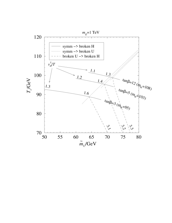
Figure 2: The perturbative phase structure using the parametrization in Eq. (3.13), together with the 2-loop Landau gauge vev $v_{H}^{L}/T$ in the broken phase.

4 Observables in 3d and 4d

Before going to simulations, let us discuss how the physical observables to be measured in 3d are related to the corresponding 4d observables.

Consider first the Higgs field vacuum expectation value $v_{H}$. This is the object by which one usually characterizes whether the phase transition is strong enough for baryogenesis [1, 2], the requirement being $v_{H}/T\mathop{\raise 1.29167pt\hbox{$>$\kern-7.5pt\raise-4.73611pt\hbox{$\sim$}}}1$. As such $v_{H}$ is, however, a gauge dependent quantity. If one computes it in the Landau gauge ($v_{H}^{L}$), as is usually done, then in terms of gauge-invariant operators the same expression would be non-local. On the other hand, there is a simple local gauge-invariant quantity closely related to $v_{H}$, namely $H^{\dagger}H\sim v_{H}^{2}/2$. The problem with $H^{\dagger}H$ is that being a composite operator, it gets renormalized beyond tree-level. One can consider two recipes for defining a unique scale independent object: either one considers the discontinuity of $H^{\dagger}H$ between the broken and symmetric phases, or one considers, say, the $\overline{\mbox{\rm MS}}$-regularized $H^{\dagger}H$ at the natural scale $g_{S3}^{2}$. The first option differs qualitatively from the Landau-gauge $v_{H}^{L}$ in that given $T_{c}$, it is sensitive to the value of $H^{\dagger}H$ in the symmetric phase and is thus an inherently non-perturbative quantity, contrary to $v_{H}^{L}$. Moreover, it can only be determined at the phase transition point (or the metastability region) where a discontinuity exists, unlike $v_{H}^{L}$. We thus choose the latter option which gives, in principle, a purely perturbative broken phase quantity for given $T$. Hence we define

$$\frac{v_{H}}{T} \equiv \left(2\frac{g_{S3}^{2}}{T}\left\langle\frac{H^{\dagger}H(g_{S3}^{2})}{g_{S3}^{2}}\right\rangle\right)^{1/2},$$

$$\frac{v_{U}}{T} \equiv \left(2\frac{g_{S3}^{2}}{T}\left\langle\frac{U^{\dagger}U(g_{S3}^{2})}{g_{S3}^{2}}\right\rangle\right)^{1/2}.$$ (4.1)

Note that due to a trivial rescaling with $T$, the dimension of $H^{\dagger}H$, $U^{\dagger}U$ is GeV in 3d.

Other observables needed in the study of the phase transition are the latent heat, the interface tension, and the different correlation lengths. These enter, for instance, the estimates for the nucleation and reheating temperatures (see, e.g., [17]), which are needed to decide whether $v_{H}/T$ should be taken at $T_{c}$ or some other temperature.

Consider first the latent heat. It is determined by

$$L=T_{c}\frac{d}{dT}\tilde{\Delta}p(T)_{T=T_{c}},$$ (4.2)

where $\tilde{\Delta}p(T)\equiv p_{s}(T)-p_{b}(T)$ and $p_{s},p_{b}$ are the pressures in the symmetric and broken phases, respectively. At the phase transition point, the partition function obeys

$$\frac{Z_{s}}{Z_{b}}\stackrel{{\scriptstyle\rm 4d}}{{=}}\exp(\frac{V}{T}\tilde{\Delta}p)\stackrel{{\scriptstyle\rm 3d}}{{=}}\exp(-Vg_{S3}^{6}\tilde{\Delta}\epsilon_{3}),$$ (4.3)

where $\epsilon_{3}$ is the dimensionless vacuum energy density of the 3d theory in Eq. (2.1). As such, $\epsilon_{3}$ is a divergent quantity, but its jump across a phase transition is finite, and the derivatives of the jumps with respect to different parameters are related to jumps of different operators. In particular, as only the parameters $y_{H},y_{U}$ depend on the temperature according to the parametrization in Eq. (3.13), one gets

$$\frac{L}{T_{c}^{4}} = -\frac{g_{S3}^{6}}{T_{c}^{2}}\frac{d}{dT}\tilde{\Delta}\epsilon_{3}(r,z,x_{H},x_{U},y_{H},y_{U})$$ (4.4)

$$= \frac{g_{S3}^{6}}{T_{c}^{2}}\left(\frac{dy_{H}}{dT}\Delta\left\langle\frac{H^{\dagger}H}{g_{S3}^{2}}\right\rangle+\frac{dy_{U}}{dT}\Delta\left\langle\frac{U^{\dagger}U}{g_{S3}^{2}}\right\rangle\right)_{T=T_{c}}$$

$$= \frac{g_{S3}^{2}}{T_{c}}\left(\frac{\tilde{m}_{H}^{2}}{T_{c}^{2}}\Delta\left\langle\frac{H^{\dagger}H}{g_{S3}^{2}}\right\rangle+2\frac{\tilde{m}_{U}^{2}}{T_{c}^{2}}\Delta\left\langle\frac{U^{\dagger}U}{g_{S3}^{2}}\right\rangle\right)_{T=T_{c}},$$

where $\Delta\left\langle\ldots\right\rangle\equiv-\tilde{\Delta}\left\langle\ldots\right\rangle=\left\langle\ldots\right\rangle_{b}-\left\langle\ldots\right\rangle_{s}$.

Consider then the interface tension. The interface tension is the extra free energy of a phase boundary separating two coexisting phases. Due to this extra free energy, the probability $P_{\rm min}$ of a configuration where there is such an interface, is smaller than the probability $P_{\rm max}$ for a pure phase. In 4d and 3d units, this is expressed as

$$\frac{P_{\rm min}}{P_{\rm max}}\stackrel{{\scriptstyle\rm 4d}}{{=}}\exp(-\frac{1}{T}\sigma A)\stackrel{{\scriptstyle\rm 3d}}{{=}}\exp(-\sigma_{3}Ag_{S3}^{4}).$$ (4.5)

It follows that on a lattice with periodic boundary conditions and the cross-sectional area $A=(N_{x}a)^{2}$,

$$\sigma_{3}=\frac{1}{2N_{x}^{2}(ag_{S3}^{2})^{2}}\ln\frac{P_{\rm max}}{P_{\rm min}},$$ (4.6)

where it was taken into account that the boundary conditions force there to exist at least two interfaces. According to Eq. (4.5), the physical interface tension is then

$$\frac{\sigma}{T_{c}^{3}}=\frac{g_{S3}^{4}}{T_{c}^{2}}\sigma_{3}=(1.085)^{2}\sigma_{3}.$$ (4.7)

Finally, let us discuss correlation lengths. The lowest-dimensional gauge invariant continuum operators, used for the mass measurements, are

$$\begin{array}[]{rclrcl}S_{H}&=&H^{\dagger}H,&G_{H}&=&\displaystyle{\frac{1}{4}}F^{a}_{ij}F^{a}_{ij},\\ V_{H}^{i}&=&\mathop{\rm Im}H^{\dagger}D^{w}_{i}H,&&&\\ S_{U}&=&U^{\dagger}U,&G_{U}&=&\displaystyle{\frac{1}{4}}G^{A}_{ij}G^{A}_{ij},\\ V_{U}^{i}&=&\mathop{\rm Im}U^{\dagger}D^{s}_{i}U.&&&\\ \end{array}$$ (4.8)

Note, in particular, that while there are perturbatively even massless gauge excitations in the phase with a nonzero $v_{U}$, these are confined by an unbroken SU(2) subgroup and only the SU(3) singlet excitation corresponding to $V_{U}^{i}$ is physical [45]. The real parts of $H^{\dagger}D^{w}_{i}H$, $U^{\dagger}D^{s}_{i}U$ could be used, as well, but they are expected to couple to the same excitations as $S_{H},S_{U}$. There can also be non-vanishing cross correlations between the operators, e.g. between $S_{H},S_{U}$, and in such a case the true eigenstates can be obtained by diagonalizing the correlation matrix. The correlation lengths are measured in units of $g_{S3}^{2}$, and can then be trivially converted to units of $T$.

5 The lattice action

We now discretize the theory in Eq. (2.1) with standard methods. The scalar fields are rescaled into a dimensionless form by $H^{\dagger}H\to\tilde{H}^{\dagger}\tilde{H}\beta_{H}/(2a)\equiv\tilde{H}^{\dagger}\tilde{H}g_{S3}^{2}$, $U^{\dagger}U\to\tilde{U}^{\dagger}\tilde{U}\beta_{U}/(2a)\equiv\tilde{U}^{\dagger}\tilde{U}g_{S3}^{2}$. The lattice Lagrangian is then

$${\cal L}_{\rm latt} = \beta_{S}\sum_{i<j}\left[1-{\frac{1}{3}}{\rm Re\,}{\rm Tr\,}P^{S}_{ij}\right]+\beta_{W}\sum_{i<j}\left[1-{\frac{1}{2}}{\rm Tr\,}P^{W}_{ij}\right]$$ (5.1)

$$- \beta_{H}\sum_{i}{\rm Re\,}\tilde{H}^{\dagger}({\bf x})U^{W}_{i}({\bf x})\tilde{H}({\bf x}+{\bf i})+\beta_{2}^{H}\tilde{H}^{\dagger}\tilde{H}+\beta_{4}^{H}\left(\tilde{H}^{\dagger}\tilde{H}\right)^{2}$$

$$- \beta_{U}\sum_{i}{\rm Re\,}\tilde{U}^{\dagger}({\bf x})U^{S}_{i}({\bf x})\tilde{U}({\bf x}+{\bf i})+\beta_{2}^{U}\tilde{U}^{\dagger}\tilde{U}+\beta_{4}^{U}\left(\tilde{U}^{\dagger}\tilde{U}\right)^{2}$$

$$+ \beta_{4}^{\gamma}\tilde{H}^{\dagger}\tilde{H}\,\tilde{U}^{\dagger}\tilde{U}.$$

Here $P^{S}_{ij},P^{W}_{ij}$ are the SU(3) and SU(2) plaquettes, respectively, and $U^{S}_{i}({\bf x}),U^{W}_{i}({\bf x})$ are the corresponding link matrices. The SU(2) Higgs field is conveniently expressed with a $2\times 2$ matrix parametrization:

$${\rm\tilde{H}}=\left(\matrix{\tilde{H}_{2}^{*}&\tilde{H}_{1}\cr-\tilde{H}_{1}^{*}&\tilde{H}_{2}\cr}\right)=h_{0}\sigma_{0}+i\sum_{a=1}^{3}h_{a}\sigma_{a},$$ (5.2)

where $\sigma_{0}=1$ and $\sigma_{a>0}$ are the Pauli matrices. When we write the Lagrangian (5.1) in terms of the representation (5.2), the $\tilde{H}$-terms are substituted through $\tilde{H}^{\dagger}M\tilde{H}\rightarrow{1\over 2}{\rm Tr\,}{\rm\tilde{H}}^{\dagger}M{\rm\tilde{H}}$. This is the form of the action we actually use in the simulations.

The lattice parameters appearing in Eq. (5.1) can be expressed in terms of the lattice spacing $a$ and the continuum parameters in Eq. (2.2). Let us denote

$$\beta_{S}=\frac{6}{ag_{S3}^{2}}.$$ (5.3)

Then it follows from the discretization procedure and from the relation between the $\overline{\mbox{\rm MS}}$ and lattice regularization schemes in 3d [46, 47] that

$$\beta_{W} = \frac{2\beta_{S}}{3r},\hskip 76.82234pt\beta_{4}^{\gamma}=\frac{216}{\beta_{S}^{3}}z,$$

$$\beta_{H} = \frac{12}{\beta_{S}},\hskip 82.51282pt\beta_{U}=\frac{12}{\beta_{S}},$$

$$\beta_{4}^{H} = \frac{216}{\beta_{S}^{3}}x_{H},\hskip 62.59596pt\beta_{4}^{U}=\frac{216}{\beta_{S}^{3}}x_{U},$$

$$\beta_{2}^{H} = \frac{36}{\beta_{S}}+\frac{216}{\beta_{S}^{3}}\Biggl{\{}y_{H}-\left({\frac{3}{2}}r+6x_{H}+3z\right)\frac{\Sigma}{4\pi}\frac{\beta_{S}}{6}$$

$$- \frac{1}{16\pi^{2}}\Biggl{[}\left(\frac{51}{16}r^{2}+9rx_{H}-12x_{H}^{2}+8z-3z^{2}\right)(\ln\beta_{S}+0.08849)$$

$$+4.9941r^{2}+5.2153rx_{H}+4.6358z\Biggr{]}\Biggr{\}},$$

$$\beta_{2}^{U} = \frac{36}{\beta_{S}}+\frac{216}{\beta_{S}^{3}}\Biggl{\{}y_{U}-\left({\frac{8}{3}}+8x_{U}+2z\right)\frac{\Sigma}{4\pi}\frac{\beta_{S}}{6}$$ (5.4)

$$- \frac{1}{16\pi^{2}}\Biggl{[}\left(8+\frac{64}{3}x_{U}-16x_{U}^{2}+3rz-2z^{2}\right)(\ln\beta_{S}+0.08849)$$

$$+19.633+12.362x_{U}+1.7384rz\Biggr{]}\Biggr{\}}.$$

Thus all the lattice couplings are determined, once the continuum parameters and $\beta_{S}$ have been fixed. The relations in Eq. (5.4) become exact in the continuum limit. Improvement formulas at finite lattice spacing which should remove the ${\cal O}(a)$ effects from most of the quantities have been derived in [48] (see also [49]).

To measure the observables in Eq. (4.1), one needs the relations of the $\overline{\mbox{\rm MS}}$ and lattice regularization schemes also for $H^{\dagger}H$, $U^{\dagger}U$. It follows [47] that

$$\left\langle{\frac{H^{\dagger}H(g_{S3}^{2})}{g_{S3}^{2}}}\right\rangle = \left\langle\tilde{H}^{\dagger}\tilde{H}\right\rangle-\frac{\Sigma}{12\pi}\beta_{S}-\frac{3}{16\pi^{2}}r(\ln\beta_{S}+0.66796),$$

$$\left\langle{\frac{U^{\dagger}U(g_{S3}^{2})}{g_{S3}^{2}}}\right\rangle = \left\langle\tilde{U}^{\dagger}\tilde{U}\right\rangle-\frac{\Sigma}{8\pi}\beta_{S}-\frac{1}{2\pi^{2}}(\ln\beta_{S}+0.66796).$$ (5.5)

Note that the discontinuities of $H^{\dagger}H$, $U^{\dagger}U$ are finite.

With these relations fixed, we are ready to go to simulations. Extrapolations to the infinite volume and continuum limits will then allow to determine non-perturbatively the properties of the $\overline{\mbox{\rm MS}}$ continuum theory in Eq. (2.1).

6 The Monte Carlo update algorithm

There are three basic reasons which make the lattice simulations of the theory in Eq. (5.1) quite a demanding numerical problem.

1. For the simulations to be reliable and allow an extrapolation to the infinite volume and continuum limits, the lattice spacing $a$ and the smallest linear extension $L=Na$ of the lattice must satisfy

$$a\ll\xi_{\rm min}<\xi_{\rm max}\ll Na,$$ (6.1)

where $\xi_{\rm min}$ and $\xi_{\rm max}$ are the smallest and the largest physical correlation lengths in the system. Thus a multiscale system where $\xi_{\rm min}\ll\xi_{\rm max}$, requires very large lattice sizes $N$. The present system does have many different excitations and scales, part of them proportional to $g_{S3}^{2}$ and part to $g_{W3}^{2}\ll g_{S3}^{2}$. We will measure the different correlation lengths in Sec. 7.5. It turns out that Eq. (6.1) can actually be well enough satisfied, due to the fact that the transition is quite strong. In a very weak (or second order) transition, the determination of (non-universal) observables would require much larger lattices, since some of the correlation lengths are very large. The lattices used are shown in Table 2.

2. While a strong transition makes it easier to satisfy Eq. (6.1), there is at the same time a serious new problem. Indeed, the transition can become so strong that during the Monte Carlo simulation the system does not want to tunnel from one metastable minimum to the other, especially for the large volumes needed in order to satisfy Eq. (6.1). On the other hand, one needs to probe both phases simultaneously with sufficient statistics in order to reliably determine the relative weights of the phases (important for determining the transition temperature) and the suppression of the mixed phase (necessary for interface tension measurements). To allow for sufficient tunnelings, one has to use multicanonical simulation algorithms.

3. A special feature of the Lagrangian (5.1) is that in the large $\tilde{m}_{U}$ -region both the $H$ and $U$ fields play a significant role in the transition, and both fields can become “broken”, though not at the same time. The coupled dynamics of the $H$ and $U$ fields makes the optimization of the update algorithm a delicate issue: it is only too easy to select an update move which evolves the configurations through the phase space extremely slowly. This is especially relevant in multicanonical simulations, where, as we shall see, the choice of the multicanonical order parameter becomes critical.

In the following subsections, we discuss in some detail the methods employed to meet these (partly exceptional) requirements.

6.1 The overrelaxation update

As usual in simulations of a system which undergoes a phase transition, the overrelaxation update is much more efficient in evolving the fields than the diffusive Metropolis or heat bath updates. Intuitively this is easy to understand: the overrelaxation update propagates information through the system in wave motion ($\mbox{dist.}\propto t$), whereas heat bath and Metropolis obey the diffusion equation ($\mbox{dist.}\propto t^{1/2}$). However, in order to ensure ergodicity one has to mix heat bath -type updates with overrelaxation.

We use a compound update step which consists of 4–6 overrelaxation sweeps through the lattice followed by one heat bath/Metropolis update sweep. In one sweep we first update all of the gauge fields, followed by the updates of the Higgs fields.

The gauge field update.  

Compared with the Higgs fields, both SU(2) and SU(3) gauge fields are relatively ‘inert’ with respect to the transition, i.e., their natural modes evolve much faster than the Higgs modes (the slow gauge modes arise only through the coupling to the Higgs fields). Thus, the gauge field update algorithms are not as critical as the ones for the Higgs fields. We use a gauge field update not qualitatively different from the standard SU(2) and SU(3) pure gauge updates, in spite of the hopping terms of the form ${\rm Tr\,}\Phi^{\dagger}({\bf x})U_{i}({\bf x})\Phi({\bf x}+i)$ in the action (note, however, the modifications due to the multicanonical update, Sec. 6.2). We use the conventional reflection overrelaxation and Kennedy-Pendleton heat bath [50] methods; for SU(3) the updates are done on the SU(2) subgroups of the SU(3) link matrices.

The overrelaxation of the Higgs fields.  

Efficient overrelaxation update algorithms for the Higgs fields $\tilde{H}$ and $\tilde{U}$ are essential in order to minimize the autocorrelation times. From the lattice Lagrangian (5.1) we can observe that the local action for the Higgs fields $\tilde{H}({\bf x})$ and $\tilde{U}({\bf x})$ can be written in the following generic form:

$$V[\phi({\bf x})]=-F_{a}({\bf x})\phi_{a}({\bf x})+C_{2}({\bf x})R^{2}({\bf x})+C_{4}R^{4}({\bf x}),$$ (6.2)

where $\phi$ is either $\tilde{U}$ or $\tilde{H}$, $R^{2}=\phi_{a}\phi_{a}$, and the index $a$ is understood to go through the real and imaginary parts of the components of the complex vectors separately: thus, for $\tilde{H}$, $a=1\ldots 4$, and for $\tilde{U}$, $a=1\ldots 6$. $F({\bf x})$ is the sum of the nearest-neighbor ‘force’ terms at site ${\bf x}$:

$$F({\bf x})=\beta_{H}\sum_{i=1,2,3}\bigl{[}U^{\dagger}_{i}({\bf x}-i)\phi({\bf x}-i)+U_{i}({\bf x})\phi({\bf x}+i)\big{]}.$$ (6.3)

This form seems to suggest separate update steps for the radial and SU($N$)-components of the Higgs fields. However, as already noticed in the simulations of SU(2)+Higgs systems in 3 and 4 dimensions [26, 32], it is much more efficient to perform an update which simultaneously modifies the radial component and the direction of the Higgs fields.

In our Higgs field update we generalize the Cartesian overrelaxation , presented in Ref. [32]: we update the Higgs variables in the plane defined by 4- or 6-dimensional vectors $\phi_{a}$ and $F_{a}$, using the components of $\phi_{a}$ parallel and perpendicular to $F_{a}$:

$$X=f_{a}\phi_{a}\,,{\hskip 14.22636pt}{\hskip 14.22636pt}Y_{a}=\phi_{a}-Xf_{a}\,,$$ (6.4)

where $f_{a}=F_{a}/F$ and $F=\sqrt{F_{a}F_{a}}$. In terms of $X$ and $Y_{a}$, Eq. (6.2) becomes

$$V(X,Y)=-XF+C_{2}\,(X^{2}+Y^{2})+2C_{4}\,X^{2}\,Y^{2}+C_{4}(X^{4}+Y^{4})\,.$$ (6.5)

The overrelaxation in $Y$ is simply the reflection $Y_{a}\rightarrow-Y_{a}$, or $\phi_{a}\rightarrow-\phi_{a}+2Xf_{a}$. For SU(2), this is exactly equivalent to the conventional reflection overrelaxation procedure. For the $X$-component, the polynomial form of $V(X)$ provides a way to perform an efficient approximate overrelaxation: we find the solution to the equation $V(X^{\prime})=V(X)$ and accept $X^{\prime}$ with the probability

$$p(X^{\prime})=\min(p_{0},1)\,,{\hskip 14.22636pt}{\hskip 14.22636pt}p_{0}={\frac{dV(X)/dX}{dV(X^{\prime})/dX^{\prime}}}\,.$$ (6.6)

Since $V(X)$ is a fourth order polynomial, solving the equation $V(X^{\prime})=V(X)$ reduces to finding the zeros of a third order polynomial (we already know one zero $X^{\prime}=X$, which can be factored out). The parameters of $V(X)$ are such that there always is only one other real root, and it is straightforward to write a closed expression for $X^{\prime}$. The update is an almost perfect overrelaxation: in our simulations the acceptance rate varies between 99.4% – 99.9% for both $\tilde{U}$ and $\tilde{H}$, depending on the $\beta_{S}$ used. The acceptance is high enough so that the “diffusive” update dynamics inherent in the Metropolis accept/reject step does not play any role, and the evolution of the field configurations is almost deterministic.

The essential part of the Cartesian overrelaxation is the $X$-component update; the update of $Y$ has only a small effect on the evolution of the fields. Intuitively, the $X$-mode update achieves its efficiency by suitably balancing the entropy and the action: in a single update move, it interpolates between states where (i) $|\Phi|$ is large and the direction is relatively parallel wrt. its neighbours and (ii) $|\Phi|$ is small and the direction more ‘randomized’. Update steps acting separately on the length and the direction of the Higgs fields do not achieve this kind of balancing, and hence the magnitude of the change in a single update can be much smaller.

6.2 The multicanonical update

The first order phase transitions are relatively strong in the whole parameter range studied in this paper. Thus, in standard simulations using the canonical ensemble, the tunnelling rate from one phase to another becomes very small at all appreciable lattice volumes. This probabilistic suppression is due to the existence of the phase interfaces in the mixed phase, and it is proportional to the interface tension times the area of the interfaces (see, for example, Fig. 6).

To enhance the probability of the mixed states we can modify the lattice action with the global  multicanonical weight function $W$:

$$S_{\rm MC}=\sum_{x}{\cal L}_{\rm latt}({\bf x})-W(R)\,,{\hskip 14.22636pt}{\hskip 14.22636pt}R=\sum_{x}r({\bf x})\,,$$ (6.7)

where $r({\bf x})$ is a suitable local order parameter sensitive to the transition. The canonical expectation value of an operator ${\cal O}$ can be calculated by reweighting the individual multicanonical measurements ${\cal O}_{k}$ with the weight function:

$$\left\langle{\cal O}\right\rangle={\sum_{k}{\cal O}_{k}e^{-W(R_{k})}}/{\sum_{k}e^{-W(R_{k})}},$$ (6.8)

where the sums go over all measurements of ${\cal O}$ and $R$. In this work we use a continuous piecewise linear parametrization for $W(R)$ (see Eq. (6.10)).

Selection of the multicanonical variable.  

The structure of the phase diagram of the theory in Eq. (5.1) is complicated enough so that the choice of a suitable multicanonical order parameter $r({\bf x})$ is, in general, not obvious. In the small $\tilde{m}_{U}$ -region the transition is driven by the SU(2) Higgs field $\tilde{H}$, and a good choice is $r=\tilde{H}^{\dagger}\tilde{H}$. This order parameter has been widely used in standard SU(2)+Higgs simulations [32, 33]. However, the situation is very different when $\tilde{m}_{U}$ becomes so large that one is near the triple point in the phase diagram (see Fig. 2): the SU(3) Higgs field $\tilde{U}$ becomes important, and $\tilde{H}^{\dagger}\tilde{H}$ is not necessarily an optimal order parameter any more. Indeed, it turns out that the selection of an optimized multicanonical variable is essential for the performance of the algorithm. In the following we discuss the different choices used for the variable.

Figure 3: The emergence of the triple point: the joint probability distribution of the SU(2) and SU(3) Higgs field lengths squared, $\tilde{H}^{\dagger}\tilde{H}$ and $\tilde{U}^{\dagger}\tilde{U}$, at $\tilde{m}_{U}=67.05$ GeV, $T=84.3$ GeV, on a $12^{3}$, $\beta_{S}=12$ lattice. Here $\left\langle{\cal O}\right\rangle\equiv\sum_{x}{\cal O}({\bf x})/V$. The three peaks correspond, from left to right, to broken $\tilde{H}$, symmetric, and broken $\tilde{U}$ phases. The relative strength of the transitions is evident from the suppression of the probability density between the peaks. When the volume is increased, the suppression between the peaks grows and the peaks become sharper.

Figure 4: One-dimensional probability distributions for the system shown in Fig. 3. Left:  the distribution of $\tilde{H}^{\dagger}\tilde{H}=\sum_{x}\tilde{H}^{\dagger}\tilde{H}({\bf x})/V$. The left peak corresponds both to the symmetric phase and the broken $U$ phase, the right peak to the broken $H$ phase. Right:  the probability distribution of $(V_{H}-V_{U})$, where $V_{H}$ and $V_{U}$ are the SU(2) and SU(3) hopping terms without the Higgs field radius, Eq. (6.9). The three phases are clearly separated: from left to right, the peaks correspond to the broken $U$, symmetric, and broken $H$ phases.

In Fig. 3 we show the joint probability distribution of $\tilde{H}^{\dagger}\tilde{H}$ and $\tilde{U}^{\dagger}\tilde{U}$ near the triple point, i.e., the coexistence point of the symmetric, broken $H$, and broken $U$ phases. The distribution is from an $\tilde{m}_{U}=67.05$ GeV, $T=84.3$ GeV, volume $12^{3}$, $\beta_{S}=12$ lattice. The appearance of three peaks in the probability distribution is clearly visible. The peak corresponding to the broken $H$ phase is strongly separated from the symmetric phase and broken $U$ phase peaks, whereas there is only a mild suppression between the broken $U$ and symmetric phase peaks. This is a clear signal of the strong first order transition between the broken $H$ and symmetric phases, and relatively much weaker transition between the broken $U$ and symmetric phases. The broken phases are connected only through the symmetric phase.

From this figure one can already see that $\tilde{H}^{\dagger}\tilde{H}$ does not distinguish the symmetric phase and the broken $U$ phase. Indeed, on the left panel of Fig. 4 we plot the one-dimensional probability distribution $p(\tilde{H}^{\dagger}\tilde{H})$ from the data shown in Fig. 3. The symmetric phase and the broken $U$ phase fall on the same peak in the distribution. Thus one should use some other variable which can distinguish the whole phase structure, in order to enhance also tunnellings from the broken $U$ phase to the symmetric phase.

Figure 5: Sections of the Monte Carlo time histories of the observable $V_{H}$ from simulations where the multicanonical order parameter is $\tilde{H}^{\dagger}\tilde{H}$ (top), $(\tilde{H}^{\dagger}\tilde{H}-\tilde{U}^{\dagger}\tilde{U})$ (middle) and $V_{H}-V_{U}$ (bottom).

Motivated by Fig. 3, an obvious choice would be to use a weight function of two variables, $W(\tilde{H}^{\dagger}\tilde{H},\tilde{U}^{\dagger}\tilde{U})$. While this would certainly be possible in principle, the use of a weight function with a higher than one-dimensional argument is quite cumbersome in practice and we did not attempt to do it here. Instead, we shall consider the one-dimensional weight function variables $(\tilde{H}^{\dagger}\tilde{H}-\tilde{U}^{\dagger}\tilde{U})$ and $(V_{H}-V_{U})$, where $V_{H}$ and $V_{U}$ are the Higgs field “hopping terms”, where the length of the Higgs fields has been divided out:

$$\begin{array}[]{rclll}V_{H}&=&\displaystyle{\frac{1}{3V}}\sum_{x,i}{\rm Re\,}h^{\dagger}({\bf x})U^{W}_{i}({\bf x})h({\bf x}+i)}{&\tilde{H}=R_{H}\times h,}{&|h|=1,\\ V_{U}&=&\displaystyle{\frac{1}{3V}}\sum_{x,i}{\rm Re\,}u^{\dagger}({\bf x})U^{S}_{i}({\bf x})u({\bf x}+i)}{&\tilde{U}=R_{U}\times u,}{&|u|=1.\end{array}$$ (6.9)

In contrast to the distribution $p(\tilde{H}^{\dagger}\tilde{H})$, the distribution $p(V_{H}-V_{U})$ on the right panel of Fig. 4 clearly separates the three phases. We thus expect $(V_{H}-V_{U})$ to be a much better multicanonical order parameter than (the volume average of) $\tilde{H}^{\dagger}\tilde{H}$. Indeed, in Fig. 5 we compare the performances of three multicanonical algorithms with weight functions $W(R)$ and variables $R=\tilde{H}^{\dagger}\tilde{H}$ (top panel), $R=\tilde{H}^{\dagger}\tilde{H}-\tilde{U}^{\dagger}\tilde{U}$ (middle panel), and $R=V_{H}-V_{U}$ (bottom panel). The time histories are from simulations of an $\tilde{m}_{U}=68$ GeV, $\beta_{S}=12$, $8^{3}$ -system at $T=83$ GeV. At these parameter values the system has a strong first order transition between the broken $H$ and broken $U$ phases. It is evident that the last multicanonical algorithm is much more efficient than the two first ones in driving the system through the transition. It should be noted that the volume $8^{3}$ used here is truly microscopic and useless for a quantitative analysis; in any reasonable volume we had trouble to make the first two algorithms to tunnel even once.

The multicanonical variable $(V_{H}-V_{U})$ depends on all of the fields on the lattice, and it has to be evaluated after each stage of the update. Why is it better than the formally simpler variable $(\tilde{H}^{\dagger}\tilde{H}-\tilde{U}^{\dagger}\tilde{U})$? One possible explanation is the fact that the probability distributions $p_{H}(\tilde{H}^{\dagger}\tilde{H})$ and $p_{U}(\tilde{U}^{\dagger}\tilde{U})$ are, by themselves, very asymmetric: they have a sharp symmetric phase peak and a broad broken phase peak (see Figs. 4, 6 and 7, for example). Remembering that in the broken $U$ -phase, $H$ is always in the symmetric peak and vice versa, and recognizing that around any single peak the probability distribution $p_{H^{-}U}(\tilde{H}^{\dagger}\tilde{H}-\tilde{U}^{\dagger}\tilde{U})$ is in essence a convolution of $p_{H}$ and $p_{U}$, we see that the distribution $p_{H-U}(x)$ has broadened peaks for both the broken $U$ and broken $H$ phases. Thus, the power of the multicanonical weight function $W(\tilde{H}^{\dagger}\tilde{H}-\tilde{U}^{\dagger}\tilde{U})$ is ‘softened’.

This can be contrasted to the probability distributions $p(V_{H})$ and $p(V_{U})$ (Fig. 6). Now both the symmetric and the broken peaks are of comparable width, and the convolution does not soften the structure of the peaks too much.

In the simulations in this paper we use two different multicanonical variables: $\tilde{H}^{\dagger}\tilde{H}$ in the small $\tilde{m}_{U}$ -region, and $(V_{H}-V_{U})$ when $\tilde{m}_{U}$ is large. Since we are using a parallel supercomputer, it is not practical to keep track of the value of the global multicanonical variable when the individual Higgs and gauge field variables are updated. We calculate the value of the multicanonical weight variable only after each global even/odd -site update sweep, and perform an accept/reject step for the whole update. Nevertheless, the change in the multicanonical variable remains small enough so that the acceptance rate is better than 90–96%, depending on volume and $\beta_{S}$.

Recursive calculation of the weight function.  

When the system has a first order phase transition, the goal is to choose the weight function $W(R)$ such that the resulting probability distribution $p_{\rm MC}(R)$ is approximately constant in the interval $R_{1}\leq R\leq R_{2}$, where $R_{1}$ and $R_{2}$ denote the pure phase peak locations. This is one of the main difficulties of the multicanonical method: a priori, the weight function is not known, and the optimal weight function is $W(R)=-\ln p_{\rm can}(R)$, where $p_{\rm can}$ is the canonical probability distribution of the observable $R$. This is one of the very quantities we attempt to determine with Monte Carlo simulations. Thus one has to use some sort of an iterative procedure for determining $W(R)$.

A precise determination of $W(R)$ is needed especially in the regime of large $\tilde{m}_{U}$, where the first order transition between the broken $H$ and $U$ phases becomes extremely strong. If we allow that the multicanonical probability distribution is ‘ideal’ up to a factor of, say, 1.5, then the multicanonical weight function must be determined with an absolute accuracy $\ln 1.5\approx 0.5$. The largest variation of $W$ in this study is $\sim 100$. (That is, we have to boost the probability of the mixed state with respect to the pure phases by a factor $\approx\exp 100$.) Thus, the weight function has to be determined to an overall relative accuracy of 0.5%. We determine the weight function with an automatized recursive process.

We parameterize $W$ with a piecewise linear continuous function:

$$W(R)=w_{i}+(w_{i+1}-w_{i}){\frac{R-R_{i}}{R_{i+1}-R_{i}}}\,,{\hskip 14.22636pt}R_{i}\leq R<R_{i+1}\,.$$ (6.10)

The $k$th estimate of the weight function is $W^{k}$, and $W^{1}$ is set to the initial estimate (it can also be a constant function). The iterative process we use here to improve on the estimate $w^{k}_{i}$ is based on the relative (canonical) probabilities $p_{i}$ that the system is in bin $(i-1)$ or $i$: then the weights are chosen so that $w_{i}-w_{i-1}=\ln(p_{i-1}/p_{i})$. In more detail, the method proceeds as follows:

(i) During a (short) run of $M$ iterations, measure

$$n^{k}_{i}=\sum_{m=1}^{M}\delta_{i}(R_{m}){\hskip 14.22636pt}\mbox{and}{\hskip 14.22636pt}h^{k}_{i}=\sum_{m=1}^{M}e^{-W^{k}(R_{m})}\delta_{i}(R_{m}),$$ (6.11)

where $\delta_{i}(R)=1$, when $R_{i-1/2}\leq R<R_{i+1/2}$, otherwise 0. Thus, $n^{k}_{i}$ is the number of ‘hits’ in the bin number $i$, and $h^{k}_{i}$ is the measured estimate of the canonical histogram.

(ii) After $k$ runs, $W^{k+1}$ can be obtained by calculating

$$w^{k+1}_{i}-w^{k+1}_{i-1}=\sum_{k^{\prime}\leq k}g^{k^{\prime}}_{i}\ln{\frac{h^{k^{\prime}}_{i-1}}{h^{k^{\prime}}_{i}}}\bigg{/}\sum_{k^{\prime}\leq k}g^{k^{\prime}}_{i},$$ (6.12)

where the function $g^{k}_{i}$ is a suitably chosen two-bin weight factor, characterizing the statistical importance of the run $k$. We use here $g^{k}_{i}=(n^{k}_{i-1}+n^{k}_{i})$, if $n^{k}_{i},n^{k}_{i-1}>n_{\rm min}$, else $g^{k}_{i}=0$. The number $n_{\rm min}\sim 10$ guarantees that the bins have some minimal amount of statistics before they are taken into account in the calculation. The initial weight function $W^{1}$ can be included in Eq. (6.12) by setting $h^{0}_{i}=\exp(-w^{1}_{i})$, and $g^{0}_{i}$ to a constant value proportional to the estimated ‘quality’ of $W^{1}$.

(iii) In practice, the convergence can be greatly accelerated by an overcorrection of $W$: let us calculate a modified weight function

$$\bar{w}^{k}_{i}=w^{k}_{i}-C\ln\sum_{k^{\prime}}n^{k^{\prime}}_{i}\,,$$ (6.13)

with a suitably chosen constant $C\sim 1$. Using now $\bar{w}^{k}_{i}$ instead of $w_{i}^{k}$ in the next round of simulations in step (i), regions of the phase space not yet frequently visited (small $\sum n^{k}_{i}$) are strongly favoured. This can dramatically accelerate the initial coverage of the whole $R$ -range of interest, and guarantees a rough estimate of the final weight function only after a modest number of iterations. Naturally, the estimate of the true weight function (which is used in the final simulations) is still given by Eq. (6.12).

(iv) The process (i)–(iii) is repeated until a good enough convergence for $W^{k}$ has been obtained.

In our simulations, the length $M$ of the runs in step (i) was 500–2000 iterations, depending on the volume, and the process (i)–(iii) was repeated $\sim 100$ times (total of 50000–150000 iterations). The whole procedure is automatized, except for the ‘exit condition’ in step (iv).

At the beginning of these set-up simulations the changes in the weight function $W$ are quite large and the system does not reach any kind of an approximate equilibrium distribution. When the run progresses, the amplitude of the modifications to $W$ decreases smoothly. These preliminary runs were only used for determining $W$, and were discarded for the analysis described below.

7 Simulations and results

Since our main interest is the phase diagram and the observables which quantify the strength of the transitions, most of our simulations were performed at and immediately around the phase transition parameters. The lattice sizes used are listed in Table 2. For each lattice listed we performed 60 000 – 200 000 compound iterations ($4\times\mbox{}$ overrelaxation + $1\times\mbox{}$heat bath). Some of the points shown include several separate runs at slightly different $T$, which are then combined with the multiple histogram reweighting.

$\tilde{m}_{U}$/GeV	$\beta_{S}$	Volumes
50	12	$12^{3}$        $16^{3}$        $20_{m}^{3}$		$12^{2}\times 36_{m}$
		$16^{2}\times 48_{m}$	$20^{2}\times 72_{m}$	$24^{2}\times 128_{m}$
	20	$16^{2}\times 64_{m}$	$20^{2}\times 72_{m}$	$24^{2}\times 72_{m}$
		$28^{2}\times 80_{m}$	$32^{2}\times 128_{m}$
60	12	$12^{3}$	$16_{m}^{3}$	$20_{m}^{3}$
		$12^{2}\times 36_{m}$	$12^{2}\times 64_{m}$	$14^{2}\times 80_{m}$
		$16^{2}\times 96_{m}$	$20^{2}\times 96_{m}$
65	12	$12^{3}$      $16_{m}^{3}$	$12^{2}\times 80_{m}$	$14^{2}\times 80_{m}$
		$16^{2}\times 80_{m}$	$20^{2}\times 80_{m}$
	20	$16^{2}\times 80_{m}$	$24^{2}\times 100_{m}$	$32^{2}\times 100_{m}$
67	12	$16^{3}$	$12^{2}\times 96_{m}$	$16^{2}\times 80_{m}$
68	12	$16^{3}$        $24^{3}$        $32^{3}$		($\mbox{symm.}\leftrightarrow\mbox{broken }U$)
		$12^{2}\times 64_{m}$	$16^{2}\times 64_{m}$	($\mbox{broken }U\leftrightarrow\mbox{broken }H$)
70	12	$12^{3}$        $16^{3}$        $24^{3}$		($\mbox{symm.}\leftrightarrow\mbox{broken }U$)
		$12_{m}^{3}$	$16_{m}^{3}$	($\mbox{broken }U\leftrightarrow\mbox{broken }H$)

Table 2: The lattice sizes and spacings used. Multicanonical simulations are marked with the subscript (_m).

A well controlled infinite volume limit is essential in order to obtain reliable results for quantities like the latent heat and interface tension. Thus, we always perform simulations with several lattice volumes at any given lattice spacing. A cylindrical lattice geometry is needed especially for the interface tension, and most of the lattices in Table 2 are highly asymmetric.

To extrapolate to the continuum limit, we have made simulations with two different lattice spacings, $\beta_{S}=12,20$, at $\tilde{m}_{U}=50$ and 65 GeV. This only allows a linear extrapolation. However, it is understood analytically that the dominant corrections are linear [48, 49], and moreover, linear extrapolations work extremely well for the case of the Standard Model [32, 38]. Note also that for the SU(2) coupling the $\beta_{S}$’s used correspond to $\beta_{W}\approx 21,35$, which are larger than the largest inverse lattice spacings used in [32, 33, 38]. We are thus confident that the linear extrapolations provide good estimates of the continuum values. Moreover, as we shall see, in several observables the lattice spacing dependence is surprisingly small.

The Monte Carlo simulations were performed on a Cray T3E parallel computer at the Center for Scientific Computing, Finland, using 32–64 nodes. The performance of the code was $\sim 105$ Mflop/second/node. The parallel communication parts of the code are based on the MILC collaboration public domain lattice QCD code [52]. The total cpu-time used was about 7.5 cpu-years of a single node’s capacity, corresponding to $\sim 2.5\times 10^{16}$ floating-point operations.

7.1 Phase diagram and critical temperatures

The critical temperature can be determined accurately from the Monte Carlo data. As in the standard electroweak model, there are no known local order parameters, which would acquire a non-zero value only in one of the phases of the model. Instead, we use quantities which display a discontinuity at the transition points (when $V\rightarrow\infty)$. The quantities we use are $\tilde{H}^{\dagger}\tilde{H}$, $\tilde{U}^{\dagger}\tilde{U}$, and the hopping terms $V_{H}$ and $V_{U}$, Eq. (6.9).

Figure 6: The pseudocritical histograms at $\tilde{m}_{U}=65$ GeV, $\beta_{S}=12$. Top:  the equal weight histograms $p(\tilde{H}^{\dagger}\tilde{H})$. Bottom:  the equal height histograms $p(V_{H})$.

Figure 7: The equal weight histograms at $\tilde{m}_{U}=68$ GeV, $\beta_{S}=12$. Top:  histograms of $\tilde{H}^{\dagger}\tilde{H}$ at the broken $U$ $\leftrightarrow$ broken $H$ transition. Bottom:  histograms of $\tilde{U}^{\dagger}\tilde{U}$ at the symmetric $\leftrightarrow$ broken $U$ transition.

For each individual lattice listed in Table 2 we locate the pseudocritical temperature $T_{c}$ with several different methods (cf. Ref. [32]):

(1) maximum of the susceptibility $\chi_{\tilde{H}^{\dagger}\tilde{H}}=V\langle(\tilde{H}^{\dagger}\tilde{H}-\langle\tilde{H}^{\dagger}\tilde{H}\rangle)^{2}\rangle$,

(2) maximum of the susceptibility $\chi_{V_{H}}=V\left\langle(V_{H}-\left\langle V_{H}\right\rangle)^{2}\right\rangle$,

(3) “equal weight” $T$-value for the distribution $p(\tilde{H}^{\dagger}\tilde{H})$,

(4) “equal height” $T$-value for the distribution $p(V_{H})$.

The items above are for transitions between the symmetric phase and the broken $H$ phase. For the symmetric $\leftrightarrow$ broken $U$ transitions we use the corresponding operators where $\tilde{H}\rightarrow\tilde{U}$. For the broken $U$ $\leftrightarrow$ broken $H$ transition we can use all of the above operators and combinations thereof. The $T_{c}$-values corresponding to the above criteria are found with the Ferrenberg-Swendsen (multi)histogram reweighting [53], and the error analysis is performed with the jackknife method, using independent reweighting for each of the jackknife blocks.

In Figs. 6 and 7 we show examples of pseudocritical histograms at $\tilde{m}_{U}=65$ GeV and 68 GeV. At $\tilde{m}_{U}=65$ GeV, the transition is between the symmetric phase and the broken $H$ phase. At $\tilde{m}_{U}=68$ GeV, there are two transitions: from the symmetric phase to the broken $U$ phase (bottom panel on Fig. 7) and from the broken $U$ phase to the broken $H$ phase (top panel). The suppression of the probability between the peaks characterizes the strength of the transitions: the symmetric $\leftrightarrow$ broken $H$ transition is a relatively strong first order transition; the symmetric $\leftrightarrow$ broken $U$ transition is much weaker; and the broken $U$ $\leftrightarrow$ broken $H$ transition is extremely strong.

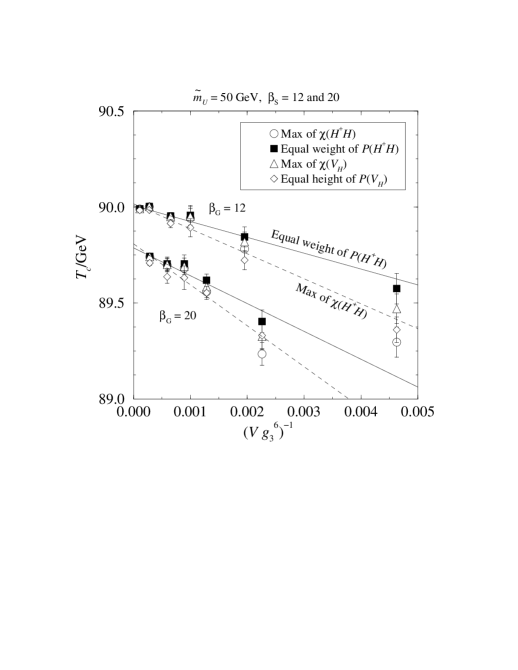
Figure 8: The infinite volume extrapolation of the critical temperature at $\tilde{m}_{U}=50$ GeV for $\beta_{S}=12$ and 20.

The infinite volume and continuum limits.  

For any given lattice the criteria (1)–(4) above yield different pseudocritical temperatures $T_{c}$. However, in the thermodynamic limit $V\rightarrow\infty$ all of the methods extrapolate very accurately to a common value. This is shown in Fig. 8 for $\tilde{m}_{U}=50$ GeV. It should be noted that the different methods do not give statistically independent results, and combining the results together is not justified. For definiteness, we use the criterion (3), the equal weight of $\tilde{H}^{\dagger}\tilde{H}$-histograms (or $\tilde{U}^{\dagger}\tilde{U}$-histograms, where appropriate), to determine our final results for $T_{c}$. In strong first order transitions the equal weight criterion is very robust, and yields practically identical results for all suitable order parameters.

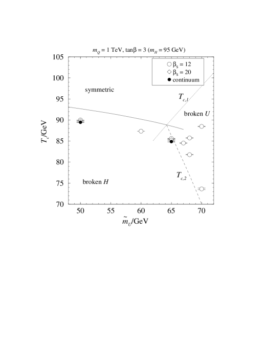
Figure 9: The phase diagram and the critical temperatures. The continuous lines are from 2-loop perturbation theory in the Landau gauge.

The results of the infinite volume extrapolations for all the different parameter values are shown in Fig. 9. For $\tilde{m}_{U}=50$ GeV and 65 GeV, we have data with two different lattice spacings, and a continuum extrapolation linear in $1/\beta_{S}=ag_{S3}^{2}/6$ is possible. The results, together with the perturbative results, are also shown in Table 3. We discuss the comparison with perturbation theory in more detail in Sec. 8.

The two different lattice spacings do not offer the possibility to check for subleading corrections in $1/\beta_{S}$. However, as already discussed in the beginning of this Section, the results from the electroweak simulations [32, 38] strongly suggest that the linear term dominates the extrapolation. It is also evident from Fig. 9 that the variations from $\beta_{S}=12$ to the continuum limit are much less than the difference from the perturbative results. Thus, even the $\beta_{S}=12$ results give a fair estimate of the continuum critical temperatures.

7.2 Scalar field expectation values

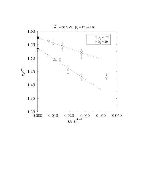
Figure 10: The infinite volume extrapolation of the $H$ field expectation value $v_{H}/T$ at $T=T_{c}$ in the broken phase, for $\tilde{m}_{U}=50$ GeV, $\beta_{S}=12$ and 20.

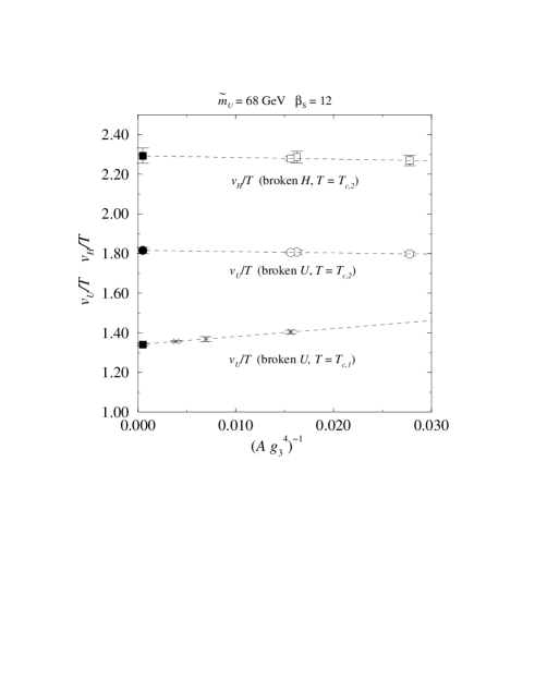
Figure 11: The infinite volume extrapolations of $v_{H}/T$ and $v_{U}/T$ at $T_{c,2}$, and $v_{U}/T$ at $T_{c,1}$, for $\tilde{m}_{U}=68$ GeV. In each case the system resides in the relevant broken phase.

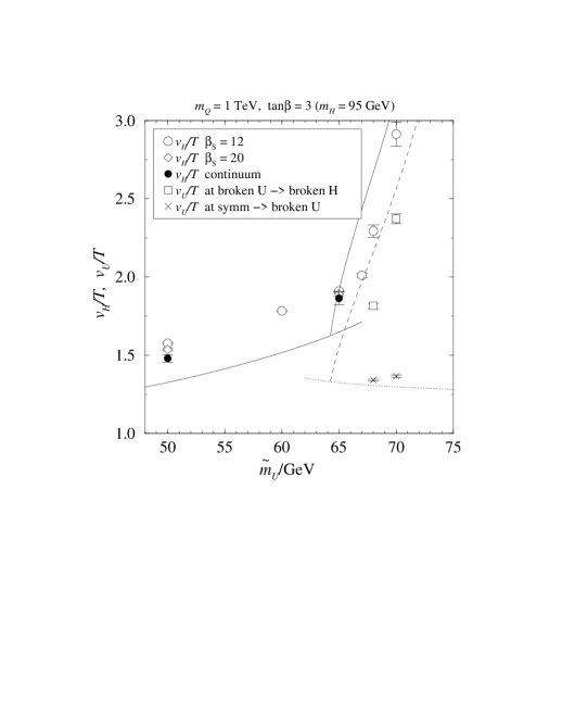
Figure 12: The scalar field expectation values in the broken phase at $T_{c}$.

The scalar field expectation values $v_{H}/T$ (in the broken $H$ phase) and $v_{U}/T$ (in the broken $U$ phase) are calculated from Eqs. (4.1) and (5.5). For this we need $\left\langle\tilde{H}^{\dagger}\tilde{H}\right\rangle$ and $\left\langle\tilde{U}^{\dagger}\tilde{U}\right\rangle$ at $T_{c}$ in the broken phase(s). These are calculated from the multicanonical results at $T_{c}$ by rejecting the symmetric phase and mixed phase measurements. This is done by imposing a suitably chosen lower cut-off for the measurements of $\tilde{H}^{\dagger}\tilde{H}$ or $\tilde{U}^{\dagger}\tilde{U}$. For example, at $\tilde{m}_{U}=65$ GeV and $\beta_{S}=12$ (Fig. 6), we accept only values $\tilde{H}^{\dagger}\tilde{H}>1.85$ (in other words, we simply calculate the center of gravity of the $\tilde{H}^{\dagger}\tilde{H}>1.85$ -part of the histogram). Since the mixed phase is very strongly suppressed, the $V\rightarrow\infty$ extrapolations are quite insensitive to the value of the cut-off.

We calculate $v_{H}/T$ and $v_{U}/T$ for each of the volumes separately, and extrapolate to the infinite volume linearly in the inverse (smallest) cross-sectional area of the lattices. As in the electroweak case [32, 38], the results from lattices of different geometries obey the $1/A$-behaviour much better than the inverse volume law. As an example, in Fig. 10 we plot $v_{H}/T$ from $\tilde{m}_{U}=50$ GeV lattices. The $V\rightarrow\infty$ extrapolations are shown in Fig. 12 and in Table 3 together with the perturbative results. For $\tilde{m}_{U}=50$ GeV and 65 GeV, we again perform the continuum extrapolation linearly in $1/\beta_{S}=a\,g^{2}_{S3}/6$.

7.3 Latent heat

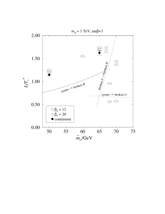
Figure 13: The infinite volume values for the latent heat.

The latent heat can be calculated from Eq. (4.4). However, in order to reduce statistical noise in the measurements, it is worthwhile to transform Eq. (4.4) into

$$\frac{L}{T_{c}^{4}}=\frac{g_{S3}^{2}}{T_{c}}\Delta\left\langle\frac{\tilde{m}_{H}^{2}}{T_{c}^{2}}\tilde{H}^{\dagger}\tilde{H}+2\frac{\tilde{m}_{U}^{2}}{T_{c}^{2}}\tilde{U}^{\dagger}\tilde{U}\right\rangle.$$ (7.1)

Here $\Delta\left\langle\ldots\right\rangle\equiv\left\langle\ldots\right\rangle_{\rm broken}-\left\langle\ldots\right\rangle_{\rm symm.}$. Eq. (7.1) implies that we measure the symmetric and broken phase expectation values of the whole expression in the angular brackets, instead of doing it for $\tilde{H}^{\dagger}\tilde{H}$ and $\tilde{U}^{\dagger}\tilde{U}$ separately.

As a function of the lattice volume and spacing, the latent heat behaves very much like the scalar field expectation values $v_{H}$ and $v_{U}$. We show the results of the $V\rightarrow\infty$ and $a\rightarrow 0$ extrapolations in Fig. 13 and in Table 3.

7.4 Interface tension

As described in Sec. 4, we measure the interface tension with the histogram method. Due to the extra free energy of the phase interfaces in the mixed phase, the probability of the mixed phase is suppressed by a factor $\propto\exp(-f_{\rm int}/T)=\exp(-\sigma A/T)$. This is seen as a ‘valley’ between the peaks corresponding to the pure phases in the order parameter histograms; see, for example, Figs. 6 and 7.

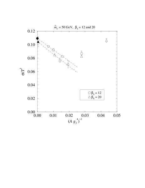
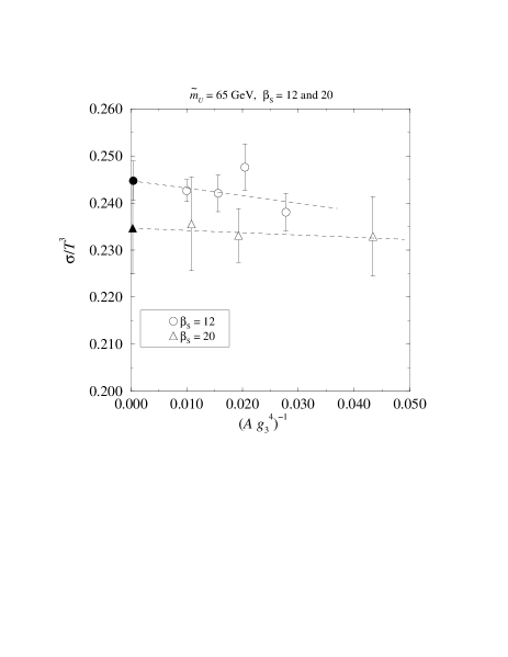
Figure 14: The $V\rightarrow\infty$ extrapolations of the interface tension for $\tilde{m}_{U}=50$ GeV (top) and 65 GeV (bottom). The values shown have been transformed with Eq. (7.2).

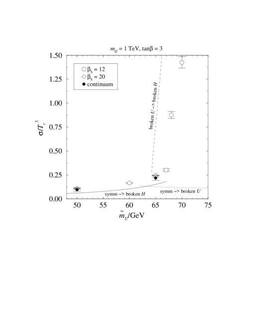
Figure 15: The infinite volume values for the interface tension.

For the interface tension measurements it is advantageous to use lattices of cylindrical geometry, $L_{z}\gg L_{x}=L_{y}$. Because of the periodic boundary conditions there are at least two interfaces which span the lattice, and because of the cylindrical geometry, they tend to form parallel to the $(x,y)$ -plane. $L_{z}$ should be then long enough that the two interfaces do not interact appreciably: this is seen as a flat minimum in the histograms.

We used the histograms $p(V_{H})$ (Eq. (6.9)) to extract the interface tension. These histograms have the advantage that they are much more symmetric than $\tilde{H}^{\dagger}\tilde{H}$ -histograms (see Fig. 6). The histograms were reweighted to the ‘equal height’ temperature. The interface tension can then be obtained from $\ln[P_{\rm max}/P_{\rm min}]/(2L^{2}_{x})\rightarrow\sigma/T$, when the volume $\rightarrow\infty$ (cf. Eq. (4.5)).

In practice, the infinite volume value of $\sigma$ is reached in such large volumes that a careful finite size analysis is necessary. Following [54, 32], we fit the data with the ansatz

$$\sigma_{3}={\frac{1}{2(L_{x}g_{S3}^{2})^{2}}}\ln{\frac{P_{\rm max}}{P_{\rm min}}}+{\frac{1}{(L_{x}g_{S3}^{2})^{2}}}\left[{\frac{3}{4}}\ln(L_{z}g^{2}_{S3})-{\frac{1}{2}}\ln(L_{x}g^{2}_{S3})+{\frac{1}{2}}G+const.\right].$$ (7.2)

The function $G$ interpolates between lattice geometries; the limiting values are $G=\ln 3$ for cubical volumes ($L_{z}=L_{x}$) and $G=0$ for long cylinders ($L_{z}\gg L_{x}$).

The results of the fit to Eq. (7.2) are shown in Fig. 14 for $\tilde{m}_{U}=50$ GeV and 65 GeV. At 50 GeV the interface tension is weak enough that we are forced to use relatively large lattices ($L_{x}>7\,g_{S3}^{-2}$) before the ansatz (7.2) can be used. In contrast, at 65 GeV we have an excellent fit to all cylindrical lattices. The small cubical lattices at $\beta_{S}=12$ do not display the flat region in the histograms and are excluded here.

The $V\rightarrow\infty$ results are shown in Fig. 15 and in Table 3. The symmetric $\leftrightarrow$ broken $U$ -transition is so weak that our volumes in Table 2 are much too small for a reliable interface tension estimate, and we did not attempt it here. In addition, at $\tilde{m}_{U}=70$ GeV at the broken $U$ $\leftrightarrow$ broken $H$ transition our lattices are too small for a reliable estimate of $\sigma$ — in this case the problem is simply that the transition is extremely strong, and the tunnelling times are very long even with the multicanonical algorithm. The largest lattice we used at $\tilde{m}_{U}=70$ GeV is $16^{3}$, and the result for $\sigma$ is to be understood only as a qualitative estimate.

$\tilde{m}_{U}$/GeV		50	60	65	67
$T_{c}$/GeV	$\beta_{S}=12$	90.0073(65)	87.347(10)	85.614(19)	84.538(23)
	$\beta_{S}=20$	89.787(16)		85.324(44)
	continuum	89.457(41)		84.89(11)
	perturb.	92.68	90.20	88.56	87.75∗
$v_{H}/T_{c}$	$\beta_{S}=12$	1.5757(49)	1.7838(47)	1.9113(57)	2.011(15)
	$\beta_{S}=20$	1.5343(89)		1.892(16)
	continuum	1.480(23)		1.864(41)
	perturb.∗∗	1.327	1.517	1.647	1.715∗
$L/T_{c}^{4}$	$\beta_{S}=12$	1.2477(62)	1.5499(88)	1.7357(34)	1.692(58)
	$\beta_{S}=20$	1.2073(91)		1.692(20)
	continuum	1.147(25)		1.626(50)
	perturb.	0.794	1.024	1.178	1.238∗
$\sigma/T_{c}^{3}$	$\beta_{S}=12$	0.1093(25)	0.1662(51)	0.2447(42)	0.301(14)
	$\beta_{S}=20$	0.1043(74)		0.2346(96)
	continuum	0.097(19)		0.219(25)
	perturb.	0.061	0.105	0.151	0.183∗
		symm. $\leftrightarrow$ broken $U$		broken $U$ $\leftrightarrow$ broken $H$
$\tilde{m}_{U}$/GeV		68	70	68	70
$T_{c}$/GeV	$\beta_{S}=12$	85.730(23)	88.471(49)	81.773(62)	73.65(19)
	perturb.	94.90	98.07	76.90	70.05
$v_{H}/T_{c}$	$\beta_{S}=12$			2.294(39)	2.914(76)
	perturb.∗∗			2.67	3.16
$v_{U}/T_{c}$	$\beta_{S}=12$	1.3415(68)	1.3663(72)	1.816(16)	2.372(31)
	perturb.∗∗	1.31	1.30	2.16	2.57
$L/T_{c}^{4}$	$\beta_{S}=12$	0.560(17)	0.571(16)	0.9570(58)	1.402(49)
	perturb.	0.668	0.663	1.434	2.041
$\sigma/T_{c}^{3}$	$\beta_{S}=12$			0.877(37)	1.426(51)
	perturb.∗∗∗			2.9	5.3

Table 3: The infinite volume and continuum extrapolations. The continuum values have been linearly extrapolated from $\beta_{S}=12,20$. The perturbative values for $\tilde{m}_{U}=67$ GeV (^∗) correspond to a transition deep in the (perturbative) metastability region, see Fig. 9. As explained in the text, it should be noted that the perturbative definitions for $v_{H}/T_{c},v_{U}/T_{c}$ (^∗∗) are not exactly the same as the non-perturbative ones. The perturbative values (^∗∗∗) for $\sigma/T_{c}^{3}$ represent an upper bound as explained in [17].

7.5 Correlation lengths

We measure the screening masses of the operators in Eqs. (4.8) from an additional series of runs at $\tilde{m}_{U}=60$ and 68 GeV, using $\beta_{S}=12$, $32^{2}\times 64$ lattices. The correlation functions are measured in the direction of the $x_{3}$-axis, and in order to enhance the projection to the ground states, we use recursive gauge invariant blocking of the fields in the $(x_{1},x_{2})$-plane. The blocking we use is similar to the one in Ref. [38]. The fields on the level $(k+1)$ are effectively defined only on the even points of the $(k)$-level lattice on the $(x,y)$-plane. The blocking is performed with the transformations (here $\phi$ is either $\tilde{H}$ or $\tilde{U}$, and $U=U^{W}$ or $U^{S}$, correspondingly)

$$\phi^{(k+1)}(y) = {\frac{1}{5}}\phi^{(k)}(x)+{\frac{1}{5}}\sum_{i=\pm 1,2}U^{(k)}_{i}(x)\phi^{(k)}(x+i),$$

$$U^{(k+1)}_{i}(y) = U^{\prime(k)}_{i}(x)U^{\prime(k)}_{i}(x+i),$$ (7.3)

$$U^{\prime(k)}_{i}(x) = {\frac{1}{3}}U^{(k)}_{i}(x)+{\frac{1}{3}}\sum_{j=\pm i^{\prime}}U^{(k)}_{j}(x)U^{(k)}_{i}(x+j)U^{(k)\dagger}_{j}(x+i),$$

where $(x_{1},x_{2},x_{3})\equiv(2y_{1},2y_{2},y_{3})$ and $i=1,2$, $i^{\prime}=3-i$. We use the blocked fields to construct the blocked SU(2) operators

$$\begin{array}[]{lrcl}\mbox{scalar:}&S^{(k)}_{H}(x)&=&\tilde{H}^{(k)\dagger}(x)\tilde{H}^{(k)}(x),\\ \mbox{vector:}&V_{H}^{i(k)}(x)&=&\mathop{\rm Im}\tilde{H}^{(k)\dagger}(x)U_{i}^{W(k)}(x)\tilde{H}^{(k)}(x+i),\\ \mbox{$0^{++}$ glueball:~{}~{}~{}}&G_{H}^{(k)}(x)&=&1-{\frac{1}{2}}{\rm Tr\,}P^{W(k)}_{12}(x),\\ \end{array}$$ (7.4)

where $P^{W}_{12}$ is the $(x_{1},x_{2})$-plane plaquette (resp. for SU(3)). The operators are summed over $(x_{1},x_{2})$-planes at each value of $x_{3}$, and we measure the plane-plane correlation functions. The operators are blocked up to 5 times, and we measure the correlation functions for each level separately. The masses are read from the exponential fall-off of these functions. Due to the periodicity in the $x_{3}$ direction, we fit a hyperbolic cosine to the vector channel and a constant + hyperbolic cosine to the scalar channel correlation functions. All of the fits use the full covariance matrix of the correlation functions. The fitting range is automatically selected so that the range is as long as possible while still keeping the confidence level acceptable.

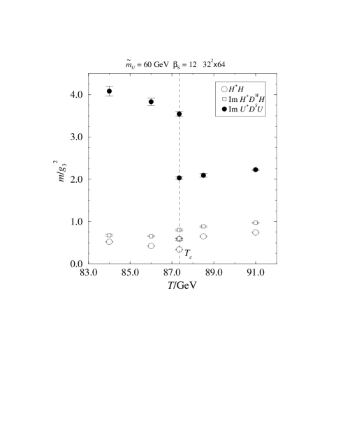
Figure 16: The screening masses at $\tilde{m}_{U}=60$ GeV, measured from a $\beta_{S}=12$, $32^{2}\times 64$ lattice. The transition temperature is marked with a vertical dashed line.

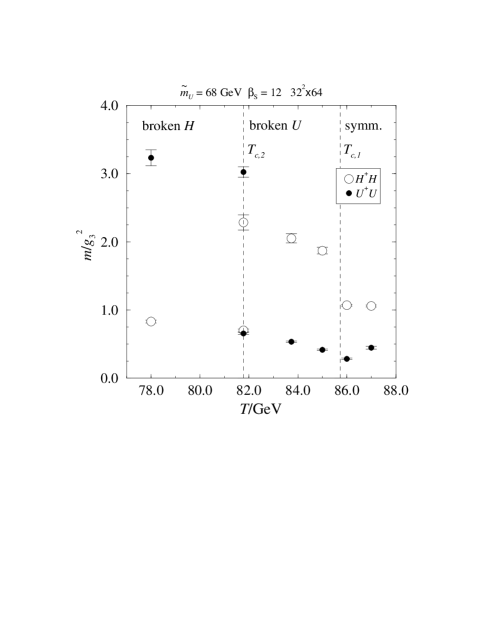
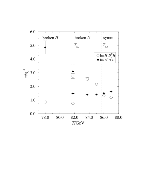
Figure 17: The screening masses at $\tilde{m}_{U}=68$ GeV, measured from a $\beta_{S}=12$, $32^{2}\times 64$ lattice. The transition temperatures are marked with the vertical dashed lines.

The screening masses for $\tilde{m}_{U}=60$ GeV are shown in Fig. 16 and for $\tilde{m}_{U}=68$ GeV in Fig. 17. For each temperature and operator we choose the blocking level which yields the best result. The optimal level was usually 4 or 5 (level 1 meaning no blocking). We observe the following:

(1) The scalar operators $S_{H}$, $S_{U}$, $G_{H}$ and $G_{U}$ all have the same quantum numbers and couple to the same set of states. A reliable measurement of the scalar mass spectrum would require the diagonalization of the full cross-correlation matrix of the scalar states, as was done for SU(2)+Higgs by Philipsen et al. [35]. Lacking the cross-correlation matrix, we were not able to reliably extract the glueball masses. Moreover, at $\tilde{m}_{U}=60$ GeV both the $S_{H}$ and $S_{U}$ operators give the mass of the lightest scalar state $S_{H}$.

(2) The vector operators do not couple to each other in a similar way, and we can measure the corresponding masses in all cases.

(3) The masses show a clear discontinuity at the critical temperatures. For $\tilde{m}_{U}=60$ GeV the behaviour of $S_{H}$ and $V^{i}_{H}$ at the transition temperature is strongly reminiscent of that for the corresponding SU(2)+Higgs theory masses [32, 35]. At the same time, the mass of the SU(3) vector state $V^{i}_{U}$ increases dramatically when the system undergoes the transition from the symmetric phase into the broken $H$ phase. This can be qualitatively understood in terms of confinement and bound states (see also [55, 56]): when the $H$-field enters the broken phase, the effective mass term of the $U$-field increases substantially, due to the $\gamma H^{\dagger}HU^{\dagger}U$ -coupling. Thus the mass of the ‘heavy squark’ meson-like bound state $U^{\dagger}U$ also increases.

8 Discussion of the results

Let us then discuss the comparison of the lattice results with perturbation theory.

The phase diagram and the critical temperatures are shown in Fig. 9. It is seen that the phase diagram is qualitatively the same as in perturbation theory, although the critical temperatures and the triple point have been displaced by a few GeV. The displacement is statistically significant, as the errors of the lattice points are very small even after continuum extrapolation. We have no clear theoretical explanation for the discrepancy between lattice results and perturbation theory: the reason might be, e.g., a three-loop perturbative effect, or a genuine non-perturbative contribution (see, e.g., [57, 58]). Let us note that the non-perturbative critical temperature for the electroweak phase transition is smaller than the perturbative one also for the Standard Model [32].

The main result of this paper is Fig. 13, which shows the latent heat. The latent heat is the most important gauge invariant physical characterization of the strength of a first order transition. We observe that the non-perturbative transition to the standard electroweak minimum at $\tilde{m}_{U}\mathop{\raise 1.29167pt\hbox{$<$\kern-7.5pt\raise-4.73611pt\hbox{$\sim$}}}67$ GeV is significantly (up to 45%) stronger than the perturbative transition. This behaviour is in strong contrast to that in the Standard Model, where the latent heat is smaller than in perturbation theory at least for Higgs masses $m_{H}\mathop{\raise 1.29167pt\hbox{$>$\kern-7.5pt\raise-4.73611pt\hbox{$\sim$}}}70$ GeV [32, 33]. Again, we have no clear explanation for this behaviour.

In the regime of the two-stage transition ($\tilde{m}_{U}\mathop{\raise 1.29167pt\hbox{$>$\kern-7.5pt\raise-4.73611pt\hbox{$\sim$}}}67$ GeV), the comparison with perturbation theory is not quite as straightforward, as the whole pattern has been shifted in $\tilde{m}_{U}$. Nevertheless, the first stage of the transition (symmetric $\to$ broken $U$) is clearly weaker than in perturbation theory, analogously to what happens for the normal transition in the Standard Model.

A similar pattern as for the latent heat, is observed for the interface tension, Fig. 15. The relative strengthening effect at $\tilde{m}_{U}\mathop{\raise 1.29167pt\hbox{$<$\kern-7.5pt\raise-4.73611pt\hbox{$\sim$}}}67$ GeV is of the same order of magnitude as for the latent heat. In the regime of large $\tilde{m}_{U}$, an important observation is that even non-perturbatively the interface tension grows very fast with increasing $\tilde{m}_{U}$. The qualitative similarity with the perturbative estimate is impressive, taking into account that the perturbative numbers shown represent a very rough upper bound estimate [17].

The scalar field expectation values are shown in Fig. 12. To get a transition strong enough for baryogenesis, one needs to have $v_{H}/T\mathop{\raise 1.29167pt\hbox{$>$\kern-7.5pt\raise-4.73611pt\hbox{$\sim$}}}1$. Again, we observe a value larger than in perturbation theory in the regime $\tilde{m}_{U}\mathop{\raise 1.29167pt\hbox{$<$\kern-7.5pt\raise-4.73611pt\hbox{$\sim$}}}67$ GeV, and a rapid increase in $v_{H}/T_{c}$ in qualitative accordance with perturbation theory in the regime of the two-stage transition, $\tilde{m}_{U}\mathop{\raise 1.29167pt\hbox{$>$\kern-7.5pt\raise-4.73611pt\hbox{$\sim$}}}67$ GeV. It should be kept in mind, though, that the definitions of the objects shown are not exactly the same in perturbation theory and on the lattice, as has been discussed in Sec. 4.

Finally, consider the correlation lengths in Figs. 16, 17. For the correlation lengths, the non-perturbative confining dynamics of the symmetric phase shows up in a very dramatic way, and comparison with perturbation theory is only possible in the broken phases. Thus, for $T<T_{c,2}$ in Fig. 17, one can compare the Higgs and SU(2) vector masses with perturbation theory, and for $T_{c,2}<T<T_{c,1}$, the stop and SU(3) vector masses. In these regimes, we observe that compared with the tree-level perturbative masses ($m_{H}/g_{S3}^{2}\sim 1.2,m_{W}/g_{S3}^{2}\sim 0.8$ for $T\mathop{\raise 1.29167pt\hbox{$<$\kern-7.5pt\raise-4.73611pt\hbox{$\sim$}}}T_{c,2}$, and $m_{\tilde{t}_{R}}/g_{S3}^{2}\sim 1.4\ldots 0.9,m_{G}/g_{S3}^{2}\sim 1.2\ldots 0.7$ for $T_{c,2}<T<T_{c,1}$), the non-perturbative scalar masses are somewhat smaller and the non-perturbative vector masses somewhat larger. This is in accordance with the pattern observed for the Standard Model in [32]. In the other regimes where the excitations feel an unbroken gauge group, the physical masses are those of bound states and very large.

9 Conclusions

We have studied the electroweak phase transition in the MSSM with non-perturbative lattice Monte Carlo simulations, in the regime of large ($m_{H}\approx 95$ GeV) Higgs masses and small ($m_{\tilde{t}_{R}}\sim 150\ldots 160$ GeV) stop masses. Several properties of the phase transition have been determined: the phase structure and critical temperatures, the latent heat, the interface tension, and the correlation lengths. The results have been extrapolated to the infinite volume and continuum limits.

The main conclusion of the study is that at least for the parameter values used, the electroweak phase transition in the MSSM is significantly stronger than indicated by 2-loop Landau-gauge $\bar{\mu}=T$ perturbation theory. If the same pattern remains there for larger Higgs masses, then this implies that previous perturbative Higgs and stop mass bounds for electroweak baryogenesis are conservative estimates. In particular, the electroweak phase transition would then be strong enough for baryogenesis for all allowed Higgs masses in this regime ($m_{H}\mathop{\raise 1.29167pt\hbox{$<$\kern-7.5pt\raise-4.73611pt\hbox{$\sim$}}}105$ GeV) [18].

This result certainly provides a strong additional motivation for experimental Higgs and stop searches at LEP and the Tevatron [18]. Moreover, it provides a strong motivation for more precise studies of the non-equilibrium CP-violating real time dynamics and baryon number generation at the electroweak phase transition. It would also be interesting (and straightforward) to extend the present simulations to other parameter values, such as a Higgs mass very close to the upper bound $m_{H}\sim 105$ GeV, and non-vanishing mixing in the squark sector. In addition, it would be useful to have an explanation for why the non-perturbative transition is stronger than indicated by 2-loop perturbation theory in the present case, in contrast to the SU(2)+Higgs model.

For the largest values of $\tilde{m}_{U}$, we have observed that the electroweak phase transition can take place in two stages, and we have analyzed this regime in detail. The values needed for $\tilde{m}_{U}$ are somewhat larger than in perturbation theory, corresponding to smaller values of $m_{\tilde{t}_{R}}$. The main physical implication of the two-stage transition is that it is a way of making the transition where the Higgs field gets a vacuum expectation value and the sphaleron rate is switched off, extremely strong. The intermediate regime where the stop field has an expectation value, might also have exotic properties.

At the same time, the price to be paid for a strong transition is that the interface tension is quite large. This implies that the supercooling taking place is significant, of order 35% already at $\tilde{m}_{U}=68$ GeV (the nucleation temperature $T_{n}$ can be estimated from $1-T_{n}/T_{c}\propto\sigma^{3/2}/(LT_{c}^{1/2})$; see, e.g, [17]). As the supercooling is getting larger, there is the danger that the transition does not take place at all during cosmological time scales, which would forbid this scenario. Thus the results can also be interpreted as an upper bound for $\tilde{m}_{U}$, or a lower bound for $m_{\tilde{t}_{R}}$ [17]. Note, however, that non-zero squark mixing parameters seem to significantly reduce the possibility of the two-stage transition [18], and at the same time they allow for smaller stop masses.

Finally, let us note that the latent heat and interface tension determined here can also be used for estimates of the non-equilibrium real-time dynamics of the transition, such as the nucleation temperature (see above), the velocities of expanding bubbles, whether reheating to $T_{c}$ takes place after the transition, etc [60]. For instance, using the non-perturbative values of $L/T_{c}^{4}$ and $\sigma/T_{c}^{3}$ for $\tilde{m}_{U}=50$ GeV, it appears that reheating to $T_{c}$ does not take place, so that the scalar vacuum expectation value after the transition is even larger than that at $T_{c}$, given in Fig. 12. This serves to further suppress the sphaleron rate.

References

- [1] V.A. Kuzmin, V.A. Rubakov and M.E. Shaposhnikov, Phys. Lett. B 155 (1985) 36; M.E. Shaposhnikov, Nucl. Phys. B 287 (1987) 757.
- [2] V.A. Rubakov and M.E. Shaposhnikov, Usp. Fiz. Nauk 166 (1996) 493 [hep-ph/9603208].
- [3] K. Kajantie, M. Laine, K. Rummukainen and M. Shaposhnikov, Phys. Rev. Lett. 77 (1996) 2887.
- [4] M. Gürtler, E.-M. Ilgenfritz and A. Schiller, Phys. Rev. D 56 (1997) 3888.
- [5] M. Giovannini and M.E. Shaposhnikov, Phys. Rev. D 57 (1998) 2186.
- [6] S. Myint, Phys. Lett. B 287 (1992) 325; G.F. Giudice, Phys. Rev. D 45 (1992) 3177.
- [7] J.R. Espinosa, M. Quirós and F. Zwirner, Phys. Lett. B 307 (1993) 106.
- [8] A. Brignole, J.R. Espinosa, M. Quirós and F. Zwirner, Phys. Lett. B 324 (1994) 181.
- [9] M. Carena, M. Quirós and C.E.M. Wagner, Phys. Lett. B 380 (1996) 81.
- [10] J.R. Espinosa, Nucl. Phys. B 475 (1996) 273.
- [11] D. Delepine, J.-M. Gérard, R. Gonzalez Felipe and J. Weyers, Phys. Lett. B 386 (1996) 183.
- [12] M. Laine, Nucl. Phys. B 481 (1996) 43 [hep-ph/9605283].
- [13] J.M. Cline and K. Kainulainen, Nucl. Phys. B 482 (1996) 73; Nucl. Phys. B 510 (1998) 88.
- [14] M. Losada, Phys. Rev. D 56 (1997) 2893; G.R. Farrar and M. Losada, Phys. Lett. B 406 (1997) 60.
- [15] J.M. Moreno, D.H. Oaknin and M. Quirós, Nucl. Phys. B 483 (1997) 267; Phys. Lett. B 395 (1997) 234.
- [16] B. de Carlos and J.R. Espinosa, Nucl. Phys. B 503 (1997) 24.
- [17] D. Bödeker, P. John, M. Laine and M.G. Schmidt, Nucl. Phys. B 497 (1997) 387 [hep-ph/9612364].
- [18] M. Carena, M. Quirós and C.E.M. Wagner, CERN-TH/97-190 [hep-ph/9710401].
- [19] M. Carena, M. Quirós, A. Riotto, I. Vilja and C.E.M. Wagner, Nucl. Phys. B 503 (1997) 387; T. Multamäki and I. Vilja, Phys. Lett. B 411 (1997) 301.
- [20] J.M. Cline, M. Joyce and K. Kainulainen, Phys. Lett. B 417 (1998) 79.
- [21] K. Enqvist, A. Riotto and I. Vilja, OUTP-97-49-P [hep-ph/9710373]; A. Riotto, CERN-TH/98-81 [hep-ph/9803357], and references therein.
- [22] M.P. Worah, Phys. Rev. D 56 (1997) 2010; Phys. Rev. Lett. 79 (1997) 3810.
- [23] J.M. Moreno, M. Quirós and M. Seco, IEM-FT-168-98 [hep-ph/9801272].
- [24] K. Funakubo, A. Kakuto, S. Otsuki and F. Toyoda, SAGA-HE-132 [hep-ph/9802276].
- [25] M. Laine and K. Rummukainen, CERN-TH/98-121 [hep-ph/9804255].
- [26] F. Csikor, Z. Fodor, J. Hein, K. Jansen, A. Jaster and I. Montvay, Phys. Lett. B 334 (1994) 405; Z. Fodor, J. Hein, K. Jansen, A. Jaster and I. Montvay, Nucl. Phys. B 439 (1995) 147; F. Csikor, Z. Fodor, J. Hein and J. Heitger, Phys. Lett. B 357 (1995) 156; F. Csikor, Z. Fodor, J. Hein, A. Jaster and I. Montvay, Nucl. Phys. B 474 (1996) 421; Y. Aoki, Phys. Rev. D 56 (1997) 3860.
- [27] P. Ginsparg, Nucl. Phys. B 170 (1980) 388; T. Appelquist and R. Pisarski, Phys. Rev. D 23 (1981) 2305; S. Nadkarni, Phys. Rev. D 27 (1983) 917.
- [28] K. Farakos, K. Kajantie, K. Rummukainen and M. Shaposhnikov, Nucl. Phys. B 425 (1994) 67; K. Kajantie, M. Laine, K. Rummukainen and M. Shaposhnikov, Nucl. Phys. B 458 (1996) 90 [hep-ph/9508379]; Phys. Lett. B, in press [hep-ph/9710538].
- [29] A. Jakovác, K. Kajantie and A. Patkós, Phys. Rev. D 49 (1994) 6810; A. Jakovác and A. Patkós, Phys. Lett. B 334 (1994) 391; Nucl. Phys. B 494 (1997) 54.
- [30] E. Braaten and A. Nieto, Phys. Rev. D 51 (1995) 6990; Phys. Rev. D 53 (1996) 3421.
- [31] K. Kajantie, K. Rummukainen and M. Shaposhnikov, Nucl. Phys. B 407 (1993) 356.
- [32] K. Kajantie, M. Laine, K. Rummukainen and M. Shaposhnikov, Nucl. Phys. B 466 (1996) 189.
- [33] E.-M. Ilgenfritz, J. Kripfganz, H. Perlt and A. Schiller, Phys. Lett. B 356 (1995) 561; M. Gürtler, E.-M. Ilgenfritz, J. Kripfganz, H. Perlt and A. Schiller, Nucl. Phys. B (Proc. Suppl.) 49 (1996) 312 [hep-lat/9512022]; Nucl. Phys. B 483 (1997) 383; M. Gürtler, E.-M. Ilgenfritz and A. Schiller, Eur. Phys. J. C 1 (1998) 363.
- [34] F. Karsch, T. Neuhaus, A. Patkós and J. Rank, Nucl. Phys. B 474 (1996) 217.
- [35] O. Philipsen, M. Teper and H. Wittig, Nucl. Phys. B 469 (1996) 445; OUTP-97-44-P [hep-lat/9709145].
- [36] G.D. Moore and N. Turok, Phys. Rev. D 55 (1997) 6538.
- [37] M. Laine and O. Philipsen, Nucl. Phys. B, in press [hep-lat/9711022].
- [38] K. Kajantie, M. Laine, K. Rummukainen and M. Shaposhnikov, Nucl. Phys. B 493 (1997) 413 [hep-lat/9612006].
- [39] T. Reisz, Z. Phys. C 53 (1992) 169; P. Lacock, D.E. Miller and T. Reisz, Nucl. Phys. B 369 (1992) 501; L. Kärkkäinen, P. Lacock, D.E. Miller, B. Petersson and T. Reisz, Phys. Lett. B 282 (1992) 121; Nucl. Phys. B 418 (1994) 3; L. Kärkkäinen, P. Lacock, B. Petersson and T. Reisz, Nucl. Phys. B 395 (1993) 733.
- [40] A. Hart, O. Philipsen, J.D. Stack and M. Teper, Phys. Lett. B 396 (1997) 217.
- [41] K. Kajantie, M. Laine, K. Rummukainen and M. Shaposhnikov, Nucl. Phys. B 503 (1997) 357 [hep-ph/9704416]; K. Kajantie, M. Laine, J. Peisa, A. Rajantie, K. Rummukainen and M. Shaposhnikov, Phys. Rev. Lett. 79 (1997) 3130 [hep-ph/9708207].
- [42] M. Karjalainen and J. Peisa, Z. Phys. C 76 (1997) 319 [hep-lat/9607023]; K. Kajantie, M. Karjalainen, M. Laine and J. Peisa, Phys. Rev. B 57 (1998) 3011 [cond-mat/9704056]; Nucl. Phys. B, in press [hep-lat/9711048]; K. Kajantie, M. Karjalainen, M. Laine, J. Peisa and A. Rajantie, Phys. Lett. B, in press [hep-ph/9803367].
- [43] P. Dimopoulos, K. Farakos and G. Koutsoumbas, Eur. Phys. J. C 1 (1998) 711.
- [44] M. Losada, to appear.
- [45] S. Dimopoulos, S. Raby and L. Susskind, Nucl. Phys. B 173 (1980) 208.
- [46] K. Farakos, K. Kajantie, K. Rummukainen, and M. Shaposhnikov, Nucl. Phys. B 442 (1995) 317 [hep-lat/9412091]; M. Laine, Nucl. Phys. B 451 (1995) 484 [hep-lat/9504001].
- [47] M. Laine and A. Rajantie, Nucl. Phys. B 513 (1998) 471 [hep-lat/9705003].
- [48] G.D. Moore, McGill-97-23 [hep-lat/9709053].
- [49] G.D. Moore, Nucl. Phys. B 493 (1997) 439; Phys. Lett. B 412 (1997) 359.
- [50] A.D. Kennedy and B.J. Pendleton, Phys. Lett. B 156 (1985) 393.
- [51] B. Berg, J. Stat. Phys. 82 (1996) 331.
- [52] The MILC collaboration public domain QCD code is available at [http://physics.indiana.edu/\̃@sg/milc.html].
- [53] A.M. Ferrenberg and R.H. Swendsen, Phys. Rev. Lett. 61 (1988) 2635.
- [54] Y. Iwasaki, K. Kanaya, L. Kärkkäinen, K. Rummukainen and T. Yoshié, Phys. Rev. D 49 (1994) 3540.
- [55] H.-G. Dosch, J. Kripfganz, A. Laser and M.G. Schmidt, Phys. Lett. B 365 (1996) 213; Nucl. Phys. B 507 (1997) 519.
- [56] W. Buchmüller and O. Philipsen, Phys. Lett. B 397 (1997) 112.
- [57] M. Shaposhnikov, Phys. Lett. B 316 (1993) 112.
- [58] S.J. Huber, A. Laser, M. Reuter and M.G. Schmidt, to appear.
- [59] G.D. Moore, McGill-97-36 [hep-ph/9801204].
- [60] H. Kurki-Suonio and M. Laine, Phys. Rev. Lett. 77 (1996) 3951.