Abstract

The square root of the positive definite hermitian operator $D_{w}^{\dagger}D_{w}$ in Neuberger’s proposal of exactly massless quarks on the lattice is implemented by the recursion formula $Y_{k+1}={1\over 2}(Y_{k}+D_{w}^{\dagger}D_{w}Y_{k}^{-1})$ with $Y_{0}=\mbox{1I}$, where $Y_{k}^{2}$ converges to $D_{w}^{\dagger}D_{w}$ quadratically. The spectrum of the lattice Dirac operator for single massless fermion in two dimensional background $U(1)$ gauge fields is investigated. For smooth background gauge fields with non-zero topological charge, the exact zero modes with definite chirality are reproduced to a very high precision on a finite lattice and the Index Theorem is satisfied exactly. The fermionic determinants are also computed and they are in good agreement with the continuum exact solution.

1 Introduction

In recent publications [1, 2], Neuberger suggested that in a vector-like gauge theory the lattice Dirac operator $D$ for exactly massless quarks can be represented by a finite matrix of fixed shape, without undesired doubling and no need for any fine tuning. The lattice Dirac fermion operator of Neuberger’s proposal of exactly massless fermion is

$$D_{h}=\mbox{1I}+V,\quad V=D_{w}(D_{w}^{\dagger}D_{w})^{-1/2}$$ (1)

where $D_{w}$ denotes the standard Wilson-Dirac lattice fermion operator with negative mass term, and $V$ is unitary ( $V^{\dagger}=V^{-1}$ ). $D_{h}$ was derived based on the observation that the overlap [3, 4, 5] for Dirac fermion in odd dimensions [6] can be written as the determinant of a finite matrix of fixed shape. The most remarkable feature of $D_{h}$ is that it satisfies the Ginsparg-Wilson relation [7]

$$D\gamma_{5}+\gamma_{5}D=D\gamma_{5}D$$ (2)

and $D_{h}$ is so far the only known $explicit$ solution of eq.(2). Ginsparg-Wilson relation was derived in 1981 as the remnant of chiral symmetry on the lattice after blocking a chirally symmetric theory with a chirality breaking local renormalization group transformation. The original Ginsparg-Wilson relation is in fact more general than eq.(2) and constitutes a matrix $R$ which is local in the position space but diagonal in the Dirac space

$$D\gamma_{5}+\gamma_{5}D=D\gamma_{5}RD$$ (3)

It serves as $the$ criterion for breaking the continuum chiral symmetry on the lattice while preserving the exact masslessness and the continuum axial anomaly. Recently, Hasenfratz, Laliena and Niedermayer [11], and Lüscher [12] explicitly showed that any $D$ satisfying the Ginsparg-Wilson relation plus some reasonable assumptions such as locality and free of species doubling must obey the Index Theorem on the lattice. Furthermore, Lüscher [12] discovered that any $D$ satisfying Ginsparg-Wilson relation implies an exact symmetry of the fermion action which may be regarded as a lattice form of chiral symmetry, reproduces the correct anomaly and the Index Theorem on the lattice. The Nielsen-Ninomiya theorem [13] can be circumvented if the continuum chiral symmetry of the fermion is replaced by the Ginsparg-Wilson relation which is the chiral symmetry realized on the lattice. Recently, Narayanan [14] has shown that the fermionic determinant of Dirac fermion operator $D$ in the form $D=\mbox{1I}+V$ and satisfying the Ginsparg-Wilson relation can be factorized into two factors which are complex conjugate of each other, corresponding to those of left-handed and right-handed Weyl fermions. This could imply that the dynamical gauge theory of $single$ massless Dirac fermion using $D_{h}$ is amenable to Hybrid Monte Carlo simulations. However, the most challenging part of Neuberger’s proposal is the implementation of the square root of the positive defintite hermitian operator $D_{w}^{\dagger}D_{w}$. The approximation of $D_{h}$ has been studied by Neuberger [15], but it sacrifices strictly masslessness. In this paper, we attempt to implement the square root operation on the positive definite hermition operator $D_{w}^{\dagger}D_{w}$ by the following recursion formula [16]

$$Y_{k+1}={1\over 2}(Y_{k}+D_{w}^{\dagger}D_{w}Y_{k}^{-1}),\quad\quad Y_{0}=\mbox{1I}$$ (4)

It can be shown that $Y_{k}^{2}$ converges to $D_{w}^{\dagger}D_{w}$ quadratically. The main purpose of this paper is to investigate the spectrum of $D_{h}$ to see to what extent this implementation can reproduce the exact zero modes with definite chirality as well as the realization of the Index Theorem on a finite lattice. The fermionic determinants are also computed and compared with the continuum exact solutions.

2 Massless Fermion Action

Neuberger’s lattice fermion operator for exactly massless fermion has been given in eq.(1). The negative mass term in the standard Wilson-Dirac lattice fermion operator $D_{w}$ can be chosen to be any value in the range $(-1,0)$. A different value of $m$ corresponds to a different renormalization for the observables. In the following, we shall restrict our discussions to the case of $m=-1$. Then the Wilson-Dirac operator becomes

$$D_{w}=-\mbox{1I}+{1\over 2}[\gamma_{\mu}(\nabla\kern-0.5pt\smash{\raise 4.5pt\hbox{$\ast$}}\kern-4.5pt_{\mu}+{\nabla_{\mu}})-\nabla\kern-0.5pt\smash{\raise 4.5pt\hbox{$\ast$}}\kern-4.5pt_{\mu}{\nabla_{\mu}}]$$ (5)

where ${\nabla_{\mu}}$ and $\nabla\kern-0.5pt\smash{\raise 4.5pt\hbox{$\ast$}}\kern-4.5pt_{\mu}$ are the forward and backward difference operators defined in the following,

$${\nabla_{\mu}}\psi(x) = \ U_{\mu}(x)\psi(x+\hat{\mu})-\psi(x)$$

$$\nabla\kern-0.5pt\smash{\raise 4.5pt\hbox{$\ast$}}\kern-4.5pt_{\mu}\psi(x) = \ \psi(x)-U_{\mu}^{\dagger}(x-\hat{\mu})\psi(x-\hat{\mu})$$

Then the lattice action of single massless fermion in background gauge field is

$$A_{h}=\sum_{x}\sum_{y}\bar{\psi}(x)D_{h}(x,y)\psi(y)$$ (6)

where the Dirac indices are suppressed.

On a torus ( $x_{\mu}\in[0,L_{\mu}],\mu=1,2$ ), the $U(1)$ gauge fields can be decomposed into global, harmonic and local parts. In this paper we use the following decomposition.

$$A_{1}(x)=-{2\pi Qx_{2}\over L_{1}L_{2}}+{2\pi h_{1}\over L_{1}}+A_{1}^{(0)}\sin({2\pi n_{2}\over L_{2}}x_{2})$$ (7)

$$A_{2}(x)={2\pi h_{2}\over L_{2}}+A_{2}^{(0)}\sin({2\pi n_{1}\over L_{1}}x_{1})$$ (8)

where the global part is characterized by the topological charge

$$Q={1\over 2\pi}\int d^{2}xF_{12}$$ (9)

which must be an integer. The harmonic parts are parameterized by two constants $h_{1}$ and $h_{2}$. The local parts are chosen to be sinusoidal fluctuatations with amplitudes $A_{1}^{(0)}$ and $A_{2}^{(0)}$ and frequencies ${2\pi n_{2}\over L_{2}}$ and ${2\pi n_{1}\over L_{1}}$ where $n_{1}$ and $n_{2}$ are integers. The discontinuity of $A_{1}(x)$ at $x_{2}=L_{2}$ due to the global part only amounts to a gauge transformation. The field strength $F_{12}=\partial_{1}A_{2}-\partial_{2}A_{1}$ is continuous on the torus. To transcribe the continuum gauge fields to the lattice, we take the lattice sites at $x_{\mu}=0,a,...,(N_{\mu}-1)a$, where $a$ is the lattice spacing and $L_{\mu}=N_{\mu}a$ is the lattice size. Then the link variables are

$$U_{1}(x) = \exp\bigl{[}{\hbox{\rm i}}A_{1}(x)a\bigr{]}$$ (10)

$$U_{2}(x) = \exp\bigl{[}{\hbox{\rm i}}A_{2}(x)a+{\hbox{\rm i}}{2\pi Qx_{1}\over L_{1}}\delta_{x_{2},(N_{2}-1)a}\bigr{]}$$ (11)

The last term in the exponent of $U_{2}(x)$ is included to ensure that the field strength $F_{12}$ which is defined by the ordered product of link variables around a plaquette is continuous on the torus.

The fermion propagator $S_{F}(x,y)$ is defined by

$$S_{F}(x,y)={1\over Z}\int\prod_{z}d\bar{\psi}(z)d\psi(z)\ {\hbox{\rm e}}^{-A_{h}}\ \psi(x)\bar{\psi}(y)$$ (12)

where

$$Z=\int\prod_{z}d\bar{\psi}(z)d\psi(z){\hbox{\rm e}}^{-A_{h}}$$ (13)

In background gauge fields of zero topological charge ( $Q=0$ ), the fermion propagator is

$$S_{F}(x,y)=D_{h}^{-1}(x,y)$$ (14)

The free fermion propagator in momentum space is

$$\tilde{S_{F}}^{(0)}(p)={a\over 2}\ \mbox{1I}-{\hbox{\rm i}}a\ {\sum_{\mu}\gamma_{\mu}\sin(p_{\mu}a)\over 2[N(p)+u(p)]}$$ (15)

where $a$ is the lattice spacing and

$$u(p)=1-\sum_{\mu}\cos(p_{\mu}a)$$ (16)

$$N(p)=\sqrt{u^{2}(p)+\sum_{\mu}\sin^{2}(p_{\mu}a)}$$ (17)

The constant term ${a\over 2}\mbox{1I}$ which vanishes in the continuum limit is expected to appear in eq.(15) such that $D_{h}^{-1}$ satisfies the Ginsparg-Wilson relation

$$\gamma_{5}D^{-1}+D^{-1}\gamma_{5}=a\gamma_{5}$$ (18)

which is equivalent to Eq.(2). The denominator $2[N(p)+u(p)]$ in eq.(15) has only one zero at $p_{1}=p_{2}=0$ for the entire Brillouin zone and its expansion around $p_{1}=p_{2}=0$ is

$$2[N(p)+u(p)]=a^{2}(p_{1}^{2}+p_{2}^{2})+O(a^{4}p^{4})$$ (19)

Therefore the free fermion propagator is free of doublers and has the correct continuum limit. We remark that it is trivial to construct $D^{-1}$ satisfying Ginsparg-Wilson relation. Any $D^{-1}$ in the form

$$D^{-1}(x,y)={a\over 2}\mbox{1I}+\sum_{\mu}\gamma_{\mu}S_{\mu}(x,y)$$ (20)

must satisfy eq.(18). However, the additional requirements that the resulting lattice fermion action $(D^{-1})^{-1}$ is local, free of species doubling and satisfying the Index Theorem would make the task rather non-trivial. So far, $D_{h}$ is the only known explicit solution fulfilling all these requirements.

3 Zero Modes and The Index Theorem

In the continuum the Dirac operator of massless fermions in a smooth background gauge field with non-zero topological charge $Q$ has zero eigenvalues and the corresponding eigenfunctions are chiral. The Index Theorem [8] asserts that the difference of the number of left-handed and right-handed zero modes is equal to the topological charge of the gauge field configuration :

$$n_{-}-n_{+}=Q$$ (21)

In two dimensions, the so called Vanishing Theorem [9] also holds :

$$Q>0 \Rightarrow n_{+}=0\quad{\hbox{\rm and }}\quad Q=n_{-}$$

$$Q<0 \Rightarrow n_{-}=0\quad{\hbox{\rm and }}\quad Q=-n_{+}$$ (22)

Recently, Hasenfratz, Laliena and Niedermayer [11], and and Lüscher [12] explicitly showed that any lattice Dirac fermion operator $D$ satisfying the Ginsparg-Wilson relation eq.(2) must obey the Index Theorem exactly. Since $D_{h}$ is an explicit solution of Ginsparg-Wilson relation, it must obey the Index Theorem exactly. However, on a finite lattice, after we implement the inverse square root operator in $D_{h}$ by the recursion formula eq.(4), it is not known a priori how the zero modes and the Index Theorem can be recovered. It turns out that even on a very small lattice ( 6 x 6 ), the exact zero modes with definite chirality are reproduced to a very high accuracy and the Index Theorem is satisfied exactly. For smooth background guage fields, the convergence of the recursion formula eq.(4) is indeed quite fast. If we require the absolute error of each matrix element satisfying the criterion

$$|Y^{2}_{ij}-(D_{w}^{\dagger}D_{w})_{ij}|<\epsilon$$ (23)

then it usually takes less than 5 iterations to reach $\epsilon=10^{-8}$ for smooth gauge configurations. For very rough configurations, the convergence could be slow and the accumulation of roundoff errors in successive iterations could cause the algorithm unstable. For exceptional configurations, $det(D_{w})=0$, then the inverse square root operator in $D_{h}$ is not defined. This is consistent with the fact that eq.(4) breaks down when $D_{w}^{\dagger}D_{w}$ is not positive definite. In fact, the convergence of eq.(4) has become very poor in the vicinities of exceptional configurations.

After the matrix $D_{h}$ is computed, we solve the following eigenproblem

$$\sum_{y}\sum_{\beta}D_{h}^{\alpha\beta}(x,y)\phi_{s}^{\beta}(y)=\lambda_{s}\phi_{s}^{\alpha}(x)\quad s=1,\cdots,2N_{1}N_{2}$$ (24)

where $x$ and $y$ are site indices, $\alpha$ and $\beta$ are Dirac indices, and $\phi_{s}$ is normalized eigenfunction

$$\sum_{x}\sum_{\alpha}[\phi_{s}^{\alpha}(x)]^{*}\phi_{s}^{\alpha}(x)=1$$ (25)

In matrix notations, these equations are rewritten as

$$D_{h}\phi_{s} = \lambda_{s}\phi_{s}$$ (26)

$$\phi_{s}^{\dagger}\phi_{s} = 1$$ (27)

Before we solve for the eigenvalues and eigenfunctions of $D_{h}$, we discuss some of their general analytical properties in the following. Since $\gamma_{5}D_{w}\gamma_{5}=D_{w}^{\dagger}$, it follows that

$$\gamma_{5}D_{h}\gamma_{5}=D_{h}^{\dagger}$$ (28)

and the secular equation

$$det(D_{h}-\lambda\mbox{1I})=det(D_{h}^{\dagger}-\lambda^{*}\mbox{1I})=det[\gamma_{5}(D_{h}-\lambda^{*}\mbox{1I})\gamma_{5}]=det(D_{h}-\lambda^{*}\mbox{1I})=0$$ (29)

implies that the eigenvalues $\lambda_{s}$ are either real or come in complex conjugate pairs. Using eq.(28) and eq.(2), we obtain

$$D_{h}^{\dagger}D_{h}=D_{h}D_{h}^{\dagger}\Longleftrightarrow D_{h}\ {{\hbox{\rm is normal }}}$$ (30)

and

$$D_{h}^{\dagger}+D_{h}=D_{h}^{\dagger}D_{h}$$ (31)

Since $D_{h}$ is normal, $D_{h}$ and $D_{h}^{\dagger}$ have common eigenfunction and their eigenvalues come in complex conjugate pairs,

$$D_{h}^{\dagger}\phi_{s}=\lambda_{s}^{*}\phi_{s}$$ (32)

and the eigenvectors $\{\phi_{s}\}$ form a complete orthonormal set. Eq.(31) implies that

$$\lambda_{s}^{*}+\lambda_{s}=\lambda_{s}^{*}\lambda_{s}\Rightarrow|\lambda_{s}-1|^{2}=1$$ (33)

Thus the eigenvalues of $D_{h}$ fall on a unit circle with center at 1 and have the reflection symmetry with respect to the real axis. We define the chirality of an eigenmode to be

$$\chi_{s}=\phi_{s}^{\dagger}\gamma_{5}\phi_{s}=\sum_{x}\sum_{\alpha}\sum_{\beta}[\phi_{s}^{\alpha}(x)]^{*}\gamma_{5}^{\alpha\beta}\phi_{s}^{\beta}(x)$$ (34)

Using eq. (28) and eq. (32), we obtain

$$D_{h}\gamma_{5}\phi_{s}=\lambda_{s}^{*}\gamma_{5}\phi_{s}$$ (35)

Multiplying $\phi_{s}^{\dagger}$ on both sides and using the eigenvalue equation, we get

$$\lambda_{s}\phi_{s}^{\dagger}\gamma_{5}\phi_{s}=\lambda_{s}^{*}\phi_{s}^{\dagger}\gamma_{5}\phi_{s}$$ (36)

Then

$$\chi_{s}=\phi_{s}^{\dagger}\gamma_{5}\phi_{s}=0\quad{\hbox{\rm if}}\ \lambda_{s}\neq\lambda_{s}^{*}$$ (37)

The chirality of any complex eigenmode is zero. If $\lambda_{s}$ is real ( 0 or 2 ), eq.(35) and eq.(26) imply that $\phi_{s}$ has definite chirality $+1$ or $-1$.

$$\gamma_{5}\phi_{s}=\pm\phi_{s}\quad{\hbox{\rm if}}\ \lambda_{s}=\lambda_{s}^{*}$$ (38)

It is remarkable that the zero modes and the +2 eigenmodes are both chiral. This is true for any $D$ satisfying the Ginsparg-Wilson relation eq. (2) and the adjoint condition eq. (28). Another useful property of chirality is that total chirality of all eigenmodes must vanish ,

$$\sum_{s}\chi_{s} = \sum_{s}\phi_{s}^{\dagger}\gamma_{5}\phi_{s}$$ (39)

$$= \sum_{s}\sum_{x}\sum_{\alpha}\sum_{\beta}[\phi_{s}^{\alpha}(x)]^{*}\gamma_{5}^{\alpha\beta}\phi_{s}^{\beta}(x)$$

$$= \sum_{x}\sum_{\alpha}\sum_{\beta}\gamma_{5}^{\alpha\beta}\delta_{\alpha\beta}=0$$

where the completeness relation

$$\sum_{s}[\phi_{s}^{\alpha}(x)]^{*}\phi_{s}^{\beta}(y)=\delta^{\alpha\beta}\delta_{xy}$$ (40)

for the eigenfunctions of $D_{h}$ has been used. From eq. (39), we immediately obtain

$$n_{2}^{+}-n_{2}^{-}=n_{-}-n_{+}$$ (41)

The sum of chirality of all +2 eigenmodes is equal to the index of the zero modes . Therefore we can identify the chirality of +2 eigenmodes as the index of the zero modes for any $D$ satisfying the Ginsparg-Wilson relation and the adjoint condition. On the other hand, the standard Wilson-Dirac lattice fermion operator $D_{w}$ satisfies the adjoint condition but not the Ginsparg-Wilson relation. The chirality of its complex eigenmodes is zero but its real eigenmodes do not have definite chirality. Moreover, it does not have exact zero modes even in a smooth background gauge field with non-zero topologically charge. Unlike those $D$ satisfying Ginsparg-Wilson relation has real eigenvalues only at 0 or 2, $D_{w}$ has real eigenvalues at several different values and the total chirality of all ( real ) eigenmodes does not vanish. Therefore, strictly speaking, we should not identify the chirality of a subset of real eigenmodes of $D_{w}$ to be the index of zero modes. Recently, Gattringer, Hip and Lang [18] conjectured that the sum of the chirality of the real eigenmodes of the Wilson-Dirac hopping matrix in the vicinity of +2D ( D is the dimensionality ) is equal to the minus of the topological charge ( $-Q$ ) of the background gauge field. However, the Wilson-Dirac fermion operator does not have exact zero modes without tuning the mass parameter for each gauge configuration. Only in the infinite volume limit, the +2D modes of Wilson-Dirac hopping matrix are equivalent to the zero modes of the Wilson-Dirac fermion operator with zero bare mass, it implies that in the infinite volume limit the approximate zero modes of the Wilson-Dirac operator will become exactly massless with definite chiralities and the Index Theorem can be satisfied exactly.

In the following we derive some basic properties of the unitary matrix $V=D_{h}-\mbox{1I}$ which has eigenvalues $\lambda_{s}-1$. The unitarity of $V$ implies that its eigenvalues are unimodular ( i.e., $e^{{\hbox{\rm i}}\theta_{s}}$ ) and the eigenvalues of $D_{h}$ are in the form $1+e^{{\hbox{\rm i}}\theta_{s}}$. The zero modes of $D_{h}$ correspond to those of eigenvalues -1 of $V$. Since the eigenvalues of V are either real ( +1 or -1 ) or come in complex conjugate pairs, it follows that

$$det(V)=(-1)^{(n_{-}+n_{+})}=(-1)^{(n_{-}-n_{+})}=(-1)^{(n_{2}^{+}-n_{2}^{-})}$$ (42)

where eq.(41) has been used in the second equality. Eq.(42) can serve as a check for the consistency of the eigenvalues.

In Table 1, the eigenvalues of $D_{h}$ are listed for $6\times 6$ lattice in the background gauge field [ eqs.(7) and (8) ] with topological charge $Q=1$; and harmonic parts with $h_{1}=0.1$ and $h_{2}=0.2$, and the local parts with $A_{1}^{(0)}=0.3$, $A_{2}^{(0)}=0.4$ and $n_{1}=n_{2}=1$. It is evident that the eigenvalues are either real ( 0 or 2 ), or come in complex conjugate pairs in a very precise manner. This property is vital to obtain real and positive fermionic determinant. There is one zero mode with exactly zero eigenvalue and chirality $-1$. Therefore we have $n_{-}=1$ and $n_{+}=0$ and the Index Theorem $Q=n_{-}-n_{+}$ is satisfied exactly. Moreover, the Vanishing Theorem $Q>0\Longleftrightarrow n_{+}=0$ which only holds in two dimensions is also satisfied. We also note that eq.(39) and eq.(41) are both satisfied. All analytical properties of the eigensystem we have discussed above are satisfied exactly. The eigenvalues in Table 1 are plotted in Fig. 1.

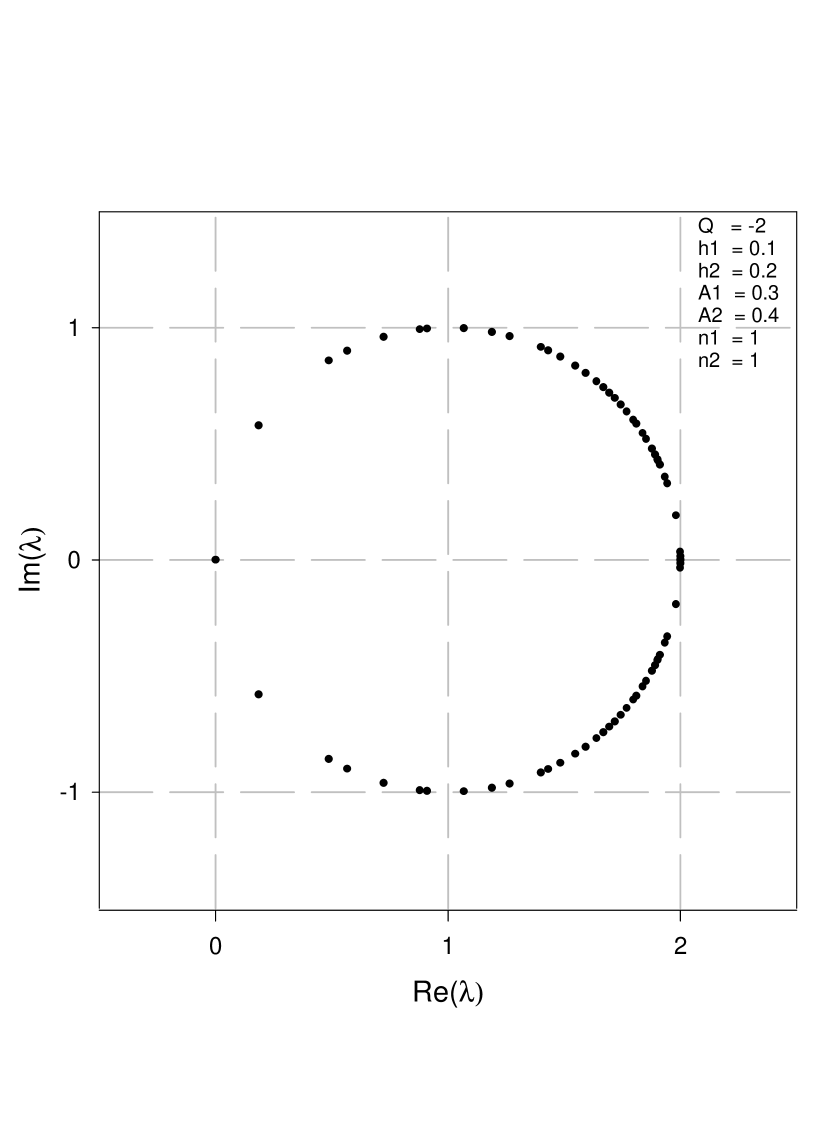
Figure 2: The eigenvalues of $D_{h}$ in Table 2.

In Table 2, the topological charge $Q=-2$ while other parameters are the same as in Table 1. There are two exact zero modes of chirality $+1$. Therefore we have $n_{-}=0$ and $n_{+}=2$ and the Index Theorem $Q=n_{-}-n_{+}$ and the Vanishing Theorem $Q<0\Longleftrightarrow n_{-}=0$ are satisfied. Again all analytical properties are satisfied exactly. The eigenvalues in Table 2 are plotted in Fig. 2.

We have tested many different smooth gauge configurations by changing the topological charge as well as other parameters in eqs. ( 7 ) and ( 8 ). The exact zero modes are always reproduced such that the Index Theorem and the Vanishing Theorem are satisfied. All analytical properties we have discussed above are satisfied exactly. We summarize some of our results in Table 3.

We also investigated the robustness of zero modes and the index theorem under local fluctuations by varying the amplitudes $A_{1}^{(0)}$ and $A_{2}^{(0)}$ as well as the frequencies ${2\pi n_{1}\over L_{1}}$ and ${2\pi n_{2}\over L_{2}}$ of the background gauge field. We found that the exact zero modes are very robust under variations of the background. For example, for $Q=1$ and $n_{1}=n_{2}=1$, the exact zero modes and the Index Theorem are reproduced for $A_{1}^{(0)}$ and $A_{2}^{(0)}$ ranging from 0.0 to 0.9.

The stability of zero modes under random fluctuations are also investigated. The rough gauge configurations are obtained from the smooth ones by multiplying each link variable with a random phase [17]

$$U_{\mu}(x)_{r}={\hbox{\rm e}}^{{\hbox{\rm i}}r\theta_{\mu}(x)}U_{\mu}(x)$$ (43)

where $\theta_{\mu}(x)$ is a uniformly distributed random variable in $(-\pi,\pi)$ and $r$ controls the size of roughness. We found that for gauge configurations with topological charge $|Q|\leq 6$ and $A_{1}^{(0)}=0.3$, $A_{2}^{(0)}=0.4$ and $n_{1}=n_{2}=1$, the exact zero modes satisfying the Index Theorem can be reproduced provided that $|r|\leq 0.3$.

Re($\lambda$)	Im($\lambda$)	chirality	Re($\lambda$)	Im($\lambda$)	chirality
2.00000000	.00000000	1.0000000
1.99981020	.01948230	.00000000	1.99981020	-.01948230	.00000000
1.98951740	.14441370	.00000000	1.98951740	-.14441370	.00000000
1.96345153	.26788272	.00000000	1.96345153	-.26788272	.00000000
1.93881783	.34441410	.00000000	1.93881783	-.34441410	.00000000
1.93303732	.35977961	.00000000	1.93303732	-.35977961	.00000000
1.93041388	.36651060	.00000000	1.93041388	-.36651060	.00000000
1.91625509	.40059533	.00000000	1.91625509	-.40059533	.00000000
1.90283899	.42997879	.00000000	1.90283899	-.42997879	.00000000
1.89600810	.44403770	.00000000	1.89600810	-.44403770	.00000000
1.87536396	.48346451	.00000000	1.87536396	-.48346451	.00000000
1.86076634	.50900030	.00000000	1.86076634	-.50900030	.00000000
1.84065148	.54157648	.00000000	1.84065148	-.54157648	.00000000
1.83027494	.55735405	.00000000	1.83027494	-.55735405	.00000000
1.80483165	.59350317	.00000000	1.80483165	-.59350317	.00000000
1.78430700	.62037289	.00000000	1.78430700	-.62037289	.00000000
1.76077457	.64901623	.00000000	1.76077457	-.64901623	.00000000
1.73598092	.67700228	.00000000	1.73598092	-.67700228	.00000000
1.71413711	.70000585	.00000000	1.71413711	-.70000585	.00000000
1.68715242	.72651329	.00000000	1.68715242	-.72651329	.00000000
1.65416649	.75635058	.00000000	1.65416649	-.75635058	.00000000
1.61565168	.78801841	.00000000	1.61565168	-.78801841	.00000000
1.57389192	.81893105	.00000000	1.57389192	-.81893105	.00000000
1.51607964	.85654060	.00000000	1.51607964	-.85654060	.00000000
1.47365734	.88070922	.00000000	1.47365734	-.88070922	.00000000
1.40247961	.91542895	.00000000	1.40247961	-.91542895	.00000000
1.30540300	.95222319	.00000000	1.30540300	-.95222319	.00000000
1.26428480	.96444468	.00000000	1.26428480	-.96444468	.00000000
1.15140180	.98847230	.00000000	1.15140180	-.98847230	.00000000
.98655620	.99990963	.00000000	.98655620	-.99990963	.00000000
.89820891	.99480580	.00000000	.89820891	-.99480580	.00000000
.78417724	.97643256	.00000000	.78417724	-.97643256	.00000000
.65832653	.93981873	.00000000	.65832653	-.93981873	.00000000
.53737749	.88655537	.00000000	.53737749	-.88655537	.00000000
.34130700	.75241181	.00000000	.34130700	-.75241181	.00000000
.10715386	.45036182	.00000000	.10715386	-.45036182	.00000000
.00000000	.00000000	-1.0000000

Table 1: The eigenvalues of $D_{h}$ in a smooth background gauge field of topological charge Q = 1. The values of other parameters are $h_{1}=0.1$, $h_{2}=0.2$, $A_{1}^{(0)}=0.3$, $A_{2}^{(0)}=0.4$ and $n_{1}=n_{2}=1$. The spectrum shows that $n_{-}=1$ , $n_{+}=0$ and the Index Theorem and Vanishing Theorem are satisfied exactly.

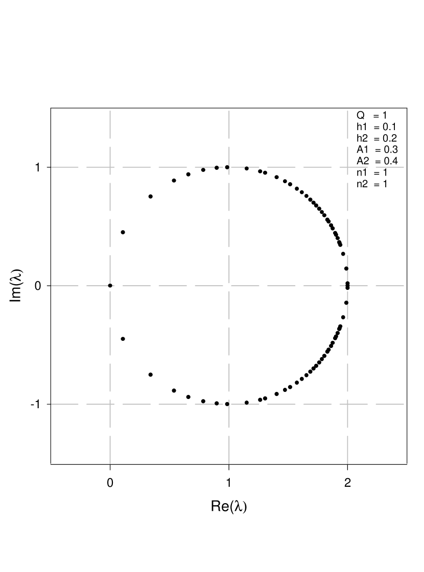
Figure 1: The eigenvalues of $D_{h}$ in Table 1.

Re($\lambda$)	Im($\lambda$)	chirality	Re($\lambda$)	Im($\lambda$)	chirality
2.00000000	.00000000	-1.0000000
2.00000000	.00000000	-1.0000000
1.99989124	.01474800	.00000000	1.99989124	-.01474800	.00000000
1.99940122	.03460068	.00000000	1.99940122	-.03460068	.00000000
1.98160401	.19092820	.00000000	1.98160401	-.19092820	.00000000
1.94402467	.32987486	.00000000	1.94402467	-.32987486	.00000000
1.93390001	.35753429	.00000000	1.93390001	-.35753429	.00000000
1.91210916	.40994742	.00000000	1.91210916	-.40994742	.00000000
1.90373008	.42810273	.00000000	1.90373008	-.42810273	.00000000
1.90165787	.43245009	.00000000	1.90165787	-.43245009	.00000000
1.89104063	.45392355	.00000000	1.89104063	-.45392355	.00000000
1.87807847	.47851667	.00000000	1.87807847	-.47851667	.00000000
1.85325494	.52149401	.00000000	1.85325494	-.52149401	.00000000
1.83821525	.54533952	.00000000	1.83821525	-.54533952	.00000000
1.81009961	.58629226	.00000000	1.81009961	-.58629226	.00000000
1.79786888	.60283103	.00000000	1.79786888	-.60283103	.00000000
1.76948744	.63866194	.00000000	1.76948744	-.63866194	.00000000
1.74331258	.66894425	.00000000	1.74331258	-.66894425	.00000000
1.71748554	.69657340	.00000000	1.71748554	-.69657340	.00000000
1.69419796	.71978413	.00000000	1.69419796	-.71978413	.00000000
1.66871002	.74352331	.00000000	1.66871002	-.74352331	.00000000
1.63944000	.76884100	.00000000	1.63944000	-.76884100	.00000000
1.59262521	.80547834	.00000000	1.59262521	-.80547834	.00000000
1.54820232	.83634575	.00000000	1.54820232	-.83634575	.00000000
1.48363430	.87527017	.00000000	1.48363430	-.87527017	.00000000
1.43095251	.90237461	.00000000	1.43095251	-.90237461	.00000000
1.39959189	.91669315	.00000000	1.39959189	-.91669315	.00000000
1.26607166	.96395325	.00000000	1.26607166	-.96395325	.00000000
1.18891548	.98199335	.00000000	1.18891548	-.98199335	.00000000
1.06804551	.99768222	.00000000	1.06804551	-.99768222	.00000000
.90949855	.99589632	.00000000	.90949855	-.99589632	.00000000
.87904797	.99265835	.00000000	.87904797	-.99265835	.00000000
.72327655	.96094960	.00000000	.72327655	-.96094960	.00000000
.56601895	.90092200	.00000000	.56601895	-.90092200	.00000000
.48688458	.85831962	.00000000	.48688458	-.85831962	.00000000
.18512327	.57963429	.00000000	.18512327	-.57963429	.00000000
.00000000	.00000000	1.0000000
.00000000	.00000000	1.0000000

Table 2: The eigenvalues of $D_{h}$ in a background gauge field of topological charge Q = -2. The values of other parameters of the gauge field are the same as in Table 1. The spectrum shows that $n_{-}=0$, $n_{+}=2$ and the Index Theorem and Vanishing Theorem are satisfied exactly.

Q	$n_{+}$	$n_{-}$	$n_{2}^{+}$	$n_{2}^{-}$
-5	5	0	0	5
-4	4	0	0	4
-3	3	0	0	3
-2	2	0	0	2
-1	1	0	0	1
0	0	0	0	0
1	0	1	1	0
2	0	2	2	0
3	0	3	3	0
4	0	4	4	0
5	0	5	5	0

Table 3: The zero modes versus the topological charge. The Index Theorem and the Vanishing Theorem are satisfied exactly. Eq.(41) is also satisfied.

4 Fermionic Determinants

The fermionic determinant $det(D)$ is proportional to the exponentiation of the one-loop effective action which is the summation of any number of external sources interacting with one internal fermion loop. It is one of the most crucial quantities to be examined in any lattice fermion formulations. The determinant of $D_{h}$ is the product of all its eigenvalues

$$det(D_{h})=\prod_{s}(1+e^{{\hbox{\rm i}}\theta_{s}})=(1+e^{{\hbox{\rm i}}\pi})^{(n_{+}+n_{-})}det_{1}(D_{h})$$ (44)

where $det_{1}(D_{h})$ is equal to the product of all non-zero eigenvalues. Since the eigenvalues are either real of come in complex conjugate pairs, $det(D_{h})$ must be real and positive. For $Q=0$, then $n_{+}+n_{-}=0$ and $det(D_{h})=det_{1}(D_{h})$. For $Q\neq 0$, then $n_{+}+n_{-}\neq 0$ and $det(D_{h})=0$, but $det_{1}(D_{h})$ still provides important information about the spectrum. In continuum, exact solutions of fermionic determinants in the general background $U(1)$ gauge fields on a torus was obtained by Sachs and Wipf [10]. In the following we compute $det_{1}(D_{h})$ for several different gauge configurations and then compare them with the exact solutions in continuum. For simplicity, we turn off the harmonic part ( $h_{1}=h_{2}=0.0$ ) and the local sinusoidal fluctuations ( $A_{1}^{(0)}=A_{2}^{(0)}=0$ ) in Eqs. (7) and (8) and examine the change of $det_{1}(D_{h})$ with respect to the topological charge $Q$. For such gauge configurations, the exact solution [10] is

$$det_{1}[D(Q)]=N\sqrt{\Bigl{(}{L_{1}L_{2}\over 2|Q|}\Bigr{)}^{|Q|}}$$ (45)

where the normalization constant $N$ is fixed by

$$N=\sqrt{\Bigl{(}{2\over L_{1}L_{2}}\Bigr{)}}$$

such that $det_{1}[D(1)]=1$.

In Table 4, the fermionic determinants $det_{1}(D_{h})$ are listed for $8\times 8$ and $16\times 16$ lattices respectively. They agree with the continuum exact solutions very well for small $Q$ but the error goes up to $10\%$ for large $Q\sim 10$. For a fixed $Q$, the error decreases with respect to the increasing of the size of the lattice.

	8 x 8		16 x 16
Q	$det_{1}[D(Q)]_{exact}$	$det_{1}[D_{h}(Q)]$	$det_{1}[D(Q)]_{exact}$	$det_{1}[D_{h}(Q)]$
1	1.00000	1.00000	1.00000	1.00000
2	2.82843	2.77348	5.65685	5.66186
3	6.15840	5.96891	24.6336	24.0615
4	11.3137	10.7157	90.5097	90.4894
5	18.3179	16.9340	293.086	286.003
6	26.8177	24.2001	858.166	822.664
7	36.1083	32.0006	2310.93	2170.94
8	45.2548	40.2920	5792.62	5354.28
9	53.2732	45.7353	13637.9	12309.5
10	59.3164	50.2816	30370.0	27336.6

Table 4: The fermionic determinant versus the topological charge $Q$. The normalization constant is chosen such that $det_{1}[D_{h}(1)]=1$. The results for the $8\times 8$ lattice are listed in the second and the third columns, while for the $16\times 16$ lattice in the last two columns. The exact solutions are computed according to Eq.( 45 ).

We have also computed the fermionic determinant $det_{1}[D_{h}]$ for more general gauge configurations with non-zero topological charge, harmonic parts and local parts; as well as in the topologically trivial sector with only harmonic parts or local parts. They are all in very good agreement with the continuum exact solutions [10].

5 Conclusions and Discussions

In this paper, we have implemented the square root operator in Neuberger’s proposal [1] of exactly massless quarks on the lattice by the recursion formula eq.(4). Our numerical tests in two dimensional background gauge fields assert that $D_{h}$ indeed reproduces the exactly massless fermions on a torus. In particular, for smooth background gauge fields with non-zero topological charge, the exact zero modes with definite chirality are reproduced and the Index Theorem is satisfied exactly.

Due to the recent work of Neuberger [1, 2], Hasenfratz, Laliena and Niedermayer [11] and Lüscher [12], we now have a better understanding of the chiral symmetry on the lattice. The Nielson-Ninomiya theorem [13] can be circumvented by replacing the continuum chiral symmetry $\{D,\gamma_{5}\}=0$ by the Ginsparg-Wilson relation $\{D,\gamma_{5}\}=D\gamma_{5}D$ on the lattice. The Ginsparg-Wilson relation gaurantees that the correct continuum anomaly can be recovered on the lattice. Currently, there are two classes of solutions satisfying the Ginsparg-Wilson relation. One of them is the explicit solution $D_{h}$ obtained by Neuberger [1], which grew out of the overlap formalism [3, 4, 5, 6]. If one attempts to solve the Ginsparg-Wilson relation by writing $D=\mbox{1I}+T$, one must end up with the solution $(\gamma_{5}T)^{2}=\mbox{1I}$. Naively one can choose any lattice operator $T$ which satisfies this condition and gives the correct continuum action in the continuum limit. The choice of $T=D_{w}(D_{w}^{\dagger}D_{w})^{-1/2}$ where $D_{w}$ is the standard Wilson-Dirac action with negative mass term is identical to Neuberger’s overlap solution. We note in passing that for any non-trivial $T$, the inverse square root operation in T seems to be inevitable . Another class of solutions of Ginsparg-Wilson relation is the fixed point lattice Dirac operator $h^{FP}$ [19] which is the implicit solution of the non-linear classical saddle-point equations, and is obtained by recursive iterations. The technical difficulty of that approach is how to parametrize $h^{FP}$ such that it is sufficiently precise but the computational costs are still affordable. It is instructive to compare our numerical results on zero modes with those obtained by Farchioni and Laliena [20] using fixed point lattice Dirac operator. It is evident that their zero modes are not exactly zero. The discrepancies are essentially due to the truncation errors in the parametrization of $h^{FP}$ and the round-off errors in the computations performed at each step of the iterations. These errors are intrinsically mixed together and therefore are very difficult to control. Furthermore, we suspect that the fermionic determinants $det_{1}(h^{FP})$ of their $h^{FP}$ would have relatively large errors. On the other hand, we do not have any serious technical difficulties to compute $D_{h}$ to a very high precision using the recursion formula eq. (4). Therefore we can obtain exact zero modes and fairly accurate fermionic determinants even on a finite lattice.

It is interesting to note that tracing the Index Theorem on the lattice has a long history. In 1987, Smit and Vink [17] investigated the spectrum of Wilson and Staggered fermions in topologically non-trivial background gauge fields in two dimensions. Some remnants of the index theorem were found but exact zero modes with definite chirality were not obtained. The Index Theorem on the lattice was also recognized by Neuberger and Narayanan [3, 21] in the context of overlap formalism. The index was computed by studying the level crossings in the spectral flow of $H(m)=\gamma_{5}D_{w}(m)$ as a function of $m$ and was verified numerically to equal to the topological charge of the background gauge field. When the lattice Dirac fermion operator $D_{h}$ was proposed by Neuberger [1], it became clear that the index computed from level crossings of $H(m)$ is equal to the index of $D_{h}$.

Although the recursion formula eq.(4) is quite effective in computing $D_{h}$ for exactly massless fermions in two dimensions, however, we expect that it would still be expensive for four dimensional lattice QCD simulations. An algorithm which invloves at most matrix multiplications but without matrix inversions at every step of iterations would be the most desirable. We are now contemplating such possibilities [22]. There are three emerging investigations that we would like to carry out in the near future. The first is the spectrum of $D_{h}$ in the four dimensional topologically non-trivial background gauge fields, which is essentially an extension of the present investigation to four dimensions [23]. The second is the quenched QCD calculations of some chirally sensitive observables such as the kaon weak matrix elements which were also calculated by Blum and Soni [24] using the Domain Wall quarks [25, 26]. Since the Domain Wall quarks in the limit of an infinite fifth dimension becomes exactly massless and is equivalent to $D_{h}$, it would be interesting to compare future results of using $D_{h}$ with those given by Domain Wall quarks with finite fifth dimension [24] and examine whether any improvements can be made by using $D_{h}$ with exactly massless quarks. The third is to perform dynamical fermion simulations of $D_{h}$ in two dimensions, for example, the Schwinger model. If the results continue to agree with the continuum exact solutions, we would attempt to confront one of the most challenging problems in QCD such as the chiral symmetry breaking by measuring the spectral density of the eigenmodes of $D_{h}$ near zero but not exactly zero.

Acknowledgement

This work is supported by the National Science Council, R.O.C. under the grant numbers NSC86-2112-M002-017 and NSC87-2112-M002-013. I wish to thank Herbert Neuberger and Sergei V. Zenkin for comments, remarks and discussions since the first version of this paper has been posed on the Web. I also wish to thank Ulli Wolff for drawing my attentions to ref. [22] and Philippe de Forcrand for suggesting a simple test on dislocations.

References

- [1] H. Neuberger, Phys. Lett. B417 (1998) 141.
- [2] H. Neuberger, ”More about exactly massless quarks on the lattice”, hep-lat/9801031.
- [3] R. Narayanan, H. Neuberger, Nucl. Phys. B 443 (1995) 305.
- [4] R. Narayanan, H. Neuberger, Phys. Lett. B 302 (1993) 62.
- [5] S. Randjbar-Daemi and J. Strathdee, Phys. Lett. B348 (1995) 543; Nucl. Phys. B443 (1995) 386; Phys. Lett. B402 (1997) 134; Nucl. Phys. B461 (1996) 305; Nucl. Phys. B466 (1996) 335.
- [6] Y. Kikukawa and H. Neuberger, Nucl. Phys. B513 (1998) 735.
- [7] P. Ginsparg and K. Wilson, Phys. Rev. D25 (1982) 2649.
- [8] M.F. Atiyah and I.M. Singer, Ann. Math. 87 (1968) 596; ibid. 93 (1971) 139.
- [9] J. Kiskis, Phys. Rev. D15 (1977) 2329; N.K. Nielson and B. Schroer, Nucl. Phys. B127 (1977) 493; M.M. Ansourian, Phys. Lett. B 70 (1977) 301.
- [10] Sachs and Wipf, Helv. Phys. Acta 65 (1992) 652.
- [11] P. Hasenfratz, V. Laliena and F. Niedermayer, ”The Index Theorem in QCD with a finite cutoff”, hep-lat/9801021.
- [12] M. Lüscher, ”Exact chiral symmetry on the lattice and the Ginsparg-Wilson relation”, hep-lat/9802011.
- [13] H.B. Nielsen and N. Ninomiya, Nucl. Phys. B185, 20 (1981); B193, 173 (1981).
- [14] R. Narayanan, ”Ginsparg-Wilson relation and the overlap formula”, hep-lat/9802018.
- [15] H. Neuberger, ”Vector like gauge theories with almost massless fermions on the lattice”, hep-lat/9710089.
- [16] G.H. Goulub and C.F. Van Loan, ” Matrix Computations ”, The Johns Hopkins University Press, 1983.
- [17] J. Smit and J. Vink, Nucl. Phys. B 286 (1987) 485.
- [18] C.R. Gattringer and I. Hip, ”On the spectrum of Wilson-Dirac lattice operator in topologically non-trivial background configurations”, hep-lat/9712015; C.R. Gattringer, I. Hip and C.B. Lang, Nucl. Phys. B (Proc. Suppl.) 63A-C (1998) 498; Nucl. Phys. B 508 (1997) 329.
- [19] P. Hasenfratz, ” The theoretical background and properties of perfect actions ” hep-lat/9803027 and references therein.
- [20] F. Farchioni and V. Laliena, ” Properties of Fixed Point Lattice Dirac Operator in the Schwinger Model ”, hep-lat/9802009.
- [21] R. Narayanan and P. Vranas, Nucl. Phys. B 506 (1997) 373.
- [22] B. Bunk, Nucl. Phys. B ( Proc. Suppl. ) 63A-C (1998) 952.
- [23] T.W. Chiu, ” Exactly Massless Fermions on the Four Dimensional Lattice ”, in preparation.
- [24] T. Blum and A. Soni, Phys. Rev. D 56, (1997) 174; Phys. Rev. Lett. 79, (1997) 3595.
- [25] D.B. Kaplan, Phys. Lett. B288 (1992) 342.
- [26] Y. Shamir, Nucl. Phys. B406 (1993) 90.