1 Introduction

As this work follows a couple of other papers which we have devoted to the study of the phase diagram of 4d simplicial gravity [2, 3], we shall not expand much on our motivations. Instead, in order to save space, we shall enter without further ado into the main body of the work. Let us only observe that following the surprising discovery [2, 4] that the phase transition between the so-called crumpled and branched polymer phases in 4d simplicial gravity is discontinuous, several groups have tried to figure out what kind of modification could render the theory more realistic. One track, explored up to now in 3d only [5, 6], consists in modifying the measure in the partition function following a recipe proposed some time ago in Ref. [7]. Loosely speaking, this corresponds to the introduction of a $R^{2}$ term in the action. Another idea consists in introducing matter fields [3]. Indeed, in the continuum formalism, one can argue that adding conformal matter fields in 4d has the effect similar to that obtained by reducing their number in 2d [10] and might therefore bring one from the branched polymer to a physical phase (analogous to the Liouville phase in 2d).

In Ref. [3] the effect of coupling non-compact $U(1)$ gauge fields to 4d simplicial quantum gravity was studied. It was found that for more than two gauge fields the back-reaction of matter on geometry is strong, that the degeneracy of random manifolds into branched polymers does not occur and that there is some evidence for a new ”smoother“ phase of the geometry, to be called hereafter the crinkled phase. This apparently confirmed the speculation put forward in [10]. The results were obtained from the strong coupling series, whose introduction in this context has been quite novel, and from Monte Carlo simulations with lattices of relatively modest size. An eventual extension of the study to larger systems was announced.

We have extended our Monte Carlo simulations to systems with up to 32K simplexes, for 3 copies of gauge fields. We have also calculated more terms of the strong coupling series. While our results are still consistent with the scenario described above, we do observe some disturbing inconsistencies in the behavior of different geometric observables which, taken at face value, seem incompatible with the existence of a single phase transition at a finite value of the Newton coupling $\kappa_{2}$.

We have noticed, on the other hand, a curious quasi-equivalence between the model with gauge fields and that with a properly modified measure. We have concentrated on this issue, achieving a better understanding of the results obtained earlier, and we have explored further both the phase structure of the model and the nature of the hypothetical crinkled phase. All these developments will be described in the following sections.

2 Gauge fields on a random manifold

The action is a sum of two parts. The first is the Einstein-Hilbert action, which for a 4d simplicial manifold reads:

$$S_{G}\,=\,-\kappa_{2}N_{2}+\kappa_{4}N_{4}\;,$$ (1)

where $N_{k}$ denotes the number of $k$-simplexes. The second part is (for one copy of the gauge field):

$$S_{M}\,=\,\sum_{t_{abc}}o(t_{abc})\left[A(l_{ab})+A(l_{bc})+A(l_{ca})\right]^{2}\;,$$ (2)

where $A(l_{ab})$ is a non-compact $U(1)$ gauge field living on link $l_{ab}$ and $A(l_{ab})$ = $-A(l_{ba})$. The sum extends over all triangles $t_{abc}$ of the random lattice and $o(t_{abc})$ denotes the order of the triangle $t_{abc}$, i.e. the number of simplexes sharing this triangle. We introduce $f$ copies of gauge fields.

Figure 1: The specific heat, $C_{V}$, and the susceptibility of the order of the most singular vertex, $\chi_{p_{0}}$, for three copies of gauge fields coupled to simplicial gravity. This is for $N_{4}$ up to 32K.

We work in a pseudo-canonical ensemble of (spherical) manifolds, with almost fixed $N_{4}$. The model is defined by the partition function:

$$Z(\kappa_{2},\bar{N}_{4})\,=\,\sum_{T}W(T)\;\int^{\prime}\prod_{l\in T}dA(l)\;\;{\rm e}^{\textstyle-S_{G}-S_{M}-\delta(N_{4}-\bar{N}_{4})^{2}}.$$ (3)

The sum is over all distinct triangulations $T$ and $W(T)$ is the symmetry factor taking care of equivalent re-labelings of vertexes. The prime indicates that the zero modes of the gauge field are not integrated. As is well known, one must allow the volume to fluctuate. The quadratic potential term added to the action ensures, for an appropriate choice of $\delta$, that these fluctuations are small. For more details see Ref. [3].

The result of our Monte Carlo simulations of the model defined by Eq. (3), for 3 copies of gauge fields, is summarized in Figure 1. There we plot both the specific heat: $C_{V}=\kappa_{2}^{2}(\langle N_{0}^{2}\rangle-\langle N_{0}\rangle^{2})/N_{4}$, and the susceptibility of the order of the most singular vertex $p_{0}$: $\chi_{p_{0}}=(\langle p_{0}^{2}\rangle-\langle p_{0}\rangle^{2})/N_{4}$. This is done for $N_{4}$ up to 32K. The specific heat has a peak at $\kappa_{2}\approx 2.5$; the location of the peak is stable but its height appears to saturate as the volume is increased. This could indicate either a continuous phase transition, of 3rd or higher order, or simply a cross-over behavior. The susceptibility $\chi_{p_{0}}$ also has a peak, rising with the volume, signaling a change in the geometry. Its location, however, moves towards larger and larger values of the coupling constant $\kappa_{2}$. As collecting data at 32K already required a considerable effort, going to a significantly larger volume is, for the moment, out of question. Thus we cannot tell whether the the location of the peak will tend to a finite value of $\kappa_{2}$ or will go to infinity.

The apparent inconsistency in the behavior of those two geometric observables — their fluctuations seem to be uncorrelated — is rather worrying. A pessimistic view is that this implies the absence of a true phase transition in the model; there will be no singularity in the infinite volume limit, and the differences in scaling behavior of the baby universe distribution and $p_{0}$ in comparison to the crumpled phase, which we have observed and which indicate a new phase, disappear in the thermodynamic limit. While our simulations cannot rule this out, another plausible explanation emerges as the phase diagram is explored in more details as we do in the next section. We will return to this discussion in the last section.

3 Modified measure

The physical variables in the partition function Eq. (3) are not the gauge fields, but the plaquette values. Let us replace in our model, for the moment without any justification, the integration over fields by the integration over plaquettes, which are by the same token assumed to fluctuate independently. They can then be integrated out, giving rise to a measure factor

$$M(T)\;\sim\;\prod_{j=1}^{N_{2}}o(t_{j})^{\beta}$$ (4)

with $\beta=-f/2$. This suggests to compare the two models, the one defined in the preceding section and that with the measure factor given by Eq. (4). We have done that leaving the parameter $\beta$ free, since it is likely that the estimate $\beta=-f/2$ is correct, if at all, in the limit $f\to\infty$ only.

Table 1: The number of different graphs $N_{g}$, for volumes $N_{4}=$ 32, 34, 36 and 38, and the corresponding weights $W_{f}(N_{4},N_{0})$. This is shown both for pure gravity, and one and three gauge fields coupled to gravity ($f=0$, 1, and 3). All weights are normalized with the value at $N_{4}=6$.

$N_{4}$	$N_{0}$	$N_{g}$	$W_{0}$	$W_{1}$	$W_{3}$
32	10	3886	2351430	$0.002787853\ldots$	$4.05397\ldots\times 10^{-21}$
	11	5943	3327045	$0.003406732\ldots$	$3.76146\ldots\times 10^{-21}$
	12	1700	6538455/8	$0.000717216\ldots$	$5.88670\ldots\times 10^{-22}$
34	10	11442	7502430	$0.002104616\ldots$	$1.72930\ldots\times 10^{-22}$
	11	26337	16396680	$0.003873112\ldots$	$2.27034\ldots\times 10^{-22}$
	12	13231	7545780	$0.001504522\ldots$	$6.40475\ldots\times 10^{-23}$
	13	922	411255	$0.000069655\ldots$	$2.14966\ldots\times 10^{-24}$
36	10	27765	18929925	$0.001231989\ldots$	$5.40586\ldots\times 10^{-24}$
	11	112097	74395157	$0.004129758\ldots$	$1.34373\ldots\times 10^{-23}$
	12	85734	54240610	$0.002520113\ldots$	$5.88459\ldots\times 10^{-24}$
	13	15298	26228930/3	$0.000339780\ldots$	$5.61994\ldots\times 10^{-25}$
38	10	71295	50097510	$0.000793825\ldots$	$2.07384\ldots\times 10^{-25}$
	11	458083	315706725	$0.004169780\ldots$	$7.73454\ldots\times 10^{-25}$
	12	490598	328515075	$0.003578606\ldots$	$4.59400\ldots\times 10^{-25}$
	13	153773	97507410	$0.000873276\ldots$	$7.72935\ldots\times 10^{-26}$
	14	6848	3781635	$0.000028143\ldots$	$1.72338\ldots\times 10^{-27}$

First we use the strong coupling series. We have extended the calculation presented in Ref. [3] up to $N_{4}=38$. The new results are summarized in Table 1. In Figure 2 we show a plot of the susceptibility exponent $\gamma$ versus $\beta$, calculated in the large–$\kappa_{2}$ phase ($\kappa_{2}=10$) using the ratio method [11]. The values of $\gamma$ are extracted assuming a large-volume behavior of the canonical partition function: $Z(N_{4})\sim\exp(\mu_{c}N_{4})N_{4}^{\gamma-3}$, where $\mu_{c}$ is the critical cosmological constant. We observe a range of (negative) couplings $\beta$ where a reliable estimate of $\gamma$ is obtained, converging as more terms of the series are included in the analysis. And, just as for the gauge field model, in this interval of $\beta$ the exponent $\gamma$ decreases continuously from the branched polymer value, $\gamma=1/2$, to a large negative value.

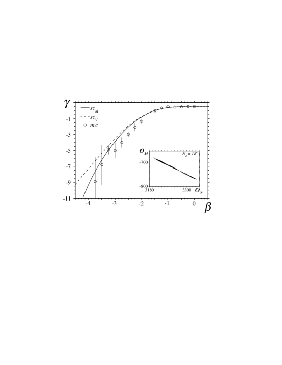
Figure 2: Variations of $\gamma$ with both the coupling $\beta$ to the measure term Eq. (4) (solid line), and with the number of gauge fields $f$ (dashed line), calculated from the series expansion. The value of $f$ has been rescaled using the relation Eq. (5). Also shown are values of $\gamma$ measured in Monte Carlo simulations with the modified measure for $\kappa_{2}=3$, varying $\beta$, on volume $N_{4}=4K$. (Insert: The correlations between the effective actions stemming from integrating out the gauge fields and from the measure term, $O_{M}$ and $O_{T}$.)

The similarity of results obtained with the two models, gauge fields and modified measure, is in fact more spectacular. In Figure 2 we also trace $\gamma$ versus $f$, making the identification

$$\beta\;=\;-\frac{f}{2}-\frac{1}{4}.$$ (5)

In an interval of the values of $\beta$ the two curves coincide! Actually, there is close agreement in the parameter range where the ratio method seems to give reliable values of $\gamma$. Note, that the leading term in Eq. (5) coincides with our earlier estimate. Of course, Eq. (5) is meaningless for too small values of $f$ ($-\beta$): there $\gamma=1/2$ for both models and the mapping is trivial.

We have further checked this remarkable equivalence in a numerical experiment, measuring the effective change to the action Eq. (1) stemming from these two seemingly unrelated modifications of the standard model. In a Monte Carlo simulation of pure gravity, with $\kappa_{2}=\beta=f=0$ and $N_{4}=1K$, we measured the effective actions:

$$O_{M}\;=\;\sum_{j}\log(o(t_{j}))\qquad{\rm and}\qquad O_{V}\;=\;\frac{1}{2}\;\log\left(\frac{\pi^{N_{1}-N_{0}+1}}{\Delta}\right),$$ (6)

where $\Delta$ is the determinant associated with the integration over one species of gauge fields. We observe a very strong linear correlation between those two observables, as shown in the insert in Figure 2. A linear fit yields a slope $-0.65$, roughly compatible with Eq. (5).

Further corroboration comes from Monte Carlo simulations at $\beta=-1.75$ (corresponding to $f=3$ in Eq. (5)), for $N_{4}=$ 4K and 8K and for $\kappa_{2}$ ranging from 0 to 4.5 . We do not wish to drown the reader in figures. It suffices to say that, up to a shift in $\kappa_{2}$ not larger than $\sim 0.5$, the results concerning the first two cumulants of $N_{0}$ and the orders of the three most singular vertexes are practically the same.

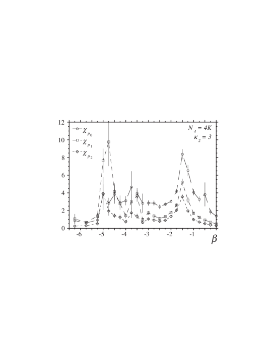
Figure 3: The fluctuations in the order of the three most singular vertexes, $p_{0}$, $p_{1}$ and $p_{2}$, for simplicial gravity with a modified measure. This is for $\kappa_{2}=3$ and volume is $N_{4}=4K$.

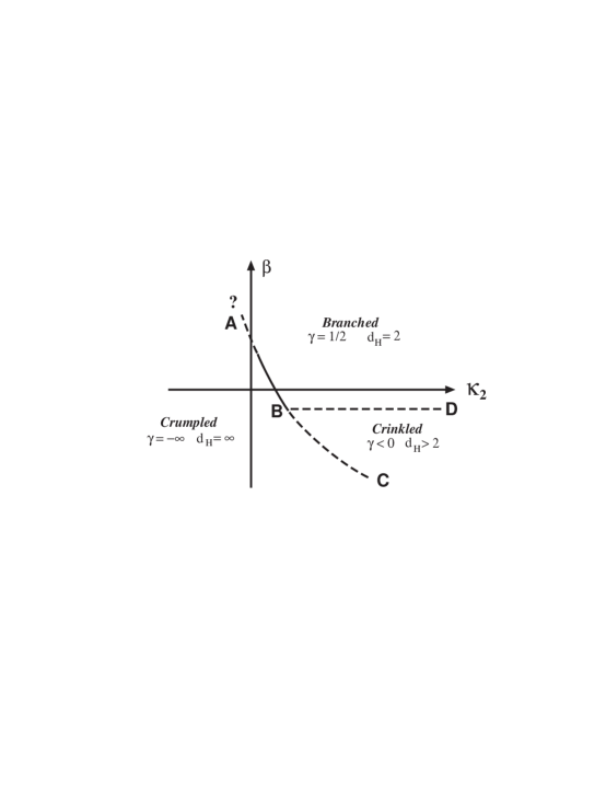
Figure 4: A schematic phase diagram of simplical gravity modified with the measure Eq. (4). At least along a portion of the line BA the phase transition is discontinuous. The same phase diagram should hold for gauge fields coupled to gravity, Eq. (3), replacing $\beta$ by the number of fields $f$ rescaled by the relation (5).

As simulating the model with a modified measure is less CPU-demanding than working with several copies of gauge fields, it has been possible to explore the phase diagram in more details. In addition, the coupling $\beta$ can be varied continuously, whereas we are restricted to integer values of $f$. We did simulations for $\kappa_{2}=3$, $N_{4}=4K$, and for several values of $\beta$. We observe strong fluctuations in geometry both at $\beta\approx-1.5$ and $\beta\approx-5$. This is indicated by peaks in the susceptibility of the various geometric observables; in Figure 4 we show this for the orders of the three most singular vertexes. The first signal corresponds roughly to the transition from branched polymers to the crinkled phase, as indicated by the series expansion, whereas the latter is a transition to a crumpled phase for $\beta\gtrsim-5$. At the moment we have only investigated this at one lattice volume, obviously further exploration is needed to establish that this indeed corresponds to two distinct transitions.

To end this section let us mention that this universality in the back-reaction on the geometry also holds for other modifications of the standard model. Using the series expansion we have investigated the effects of adding: (a) Gaussian scalar fields, (b) a discretized $R^{2}$-term as used in Ref. [8], and (c) a modified measure using a product of vertex orders. In all three cases it is possible, by an appropriate rescaling of the corresponding couplings, to map the extracted values of $\gamma$ on the curve in Figure 2, although the agreement is not as spectacular as that between the model with gauge fields and the one with a measure modified according to Eq. (4), respectively.

4 The nature of crinkled manifolds

We have explored further the nature of the hypothetical crinkled phase in Monte Carlo simulations. We have calculated the exponent $\gamma$, from the distribution of baby universes, along two lines in the phase diagram: $l_{1}=\{\kappa_{2}=3,\beta\}$ and $l_{2}=\{\kappa_{2},\beta=-3.5\}$. The values of $\gamma$ measured along $l_{1}$, included in Figure 2, agree reasonably with the predictions of the series expansion. The values of $\gamma$ measured along $l_{2}$ are shown in Table 2. For small values of $\kappa_{2}$ it is not possible to extract any reliable value. This is to be expected as the model is in the crumpled phase. For $\kappa_{2}\gtrsim 3.5$, however, we get a consistent value $\gamma\approx-4.5$, compared with the prediction of the strong coupling expansion, $\gamma\approx-6.2$, obtained for $\beta=-3.5$ and $\kappa_{2}$ large.

Table 2: Values of the string susceptibility exponent $\gamma$, measured in Monte Carlo simulations at $N_{4}=4K$, for $\beta=-3.5$ and varying $\kappa_{2}$. The series expansion predicts $\gamma\approx-6.2$, for $\beta=-3.5$ and large values of $\kappa_{2}$.

$\kappa_{2}$	$\gamma$	$\kappa_{2}$	$\gamma$
3.5	-5.75(15)	6.0	-4.71(46)
4.0	-6.24(26)	6.5	-4.19(30)
4.5	-6.23(23)	7.0	-4.27(38)
5.0	-4.41(12)	7.5	-4.14(70)
5.5	-4.42(25)

Other exponents characterizing the fractal geometry are the Hausdorff and spectral dimensions of the manifolds, $d_{H}$ and $d_{s}$. The former is related to the volume of space within a sphere of geodesic radius $r$ from a marked point: $v(r)\sim r^{d_{H}}$, whereas the spectral dimension defines the return probability for a random walker on the triangulation: $p(t)\sim t^{-d_{s}/2}$ [12]. The time $t$ is measured in units of jumps between neighboring vertexes, with hopping probability given by the inverse of the coordination number. On smooth regular manifolds those two definitions of dimensionality coincide. However, on highly fractal manifolds, like the ones that dominate the partition function Eq. (3), they are in general different.

We have extracted the Hausdorff dimension for $\kappa_{2}=4.5$ and $\beta=-1.75$ and $-3.5$, from the expected scaling behavior of the average distance between two simplexes: $\langle r_{ij}\rangle_{N_{4}}\sim N_{4}^{1/d_{H}}$. Measurements at volume $N_{4}$ = 4K to 32K were included in the fit. For $\beta=-1.75$ we got $d_{H}=3.57(16)$, which should be compared to $d_{H}=3.97(15)$ quoted in Ref. [3] for $f=3$ and $\kappa_{2}=4.5$. For $\beta=-3.5$ we got $d_{H}\approx 5$, but this estimate is less reliable.

Table 3: The extracted values of the spectral dimension $d_{s}$ for simplical gravity with a modified measure. This is for $\kappa_{2}=4.5$ and both for $\beta=0$ (branched polymer phase) and for $\beta=-1.75$ and -3.5 (crinkled phase).

$N_{4}$	$\beta=0.00$	$\beta=-1.75$	$\beta=-3.5$
2K	1.33(1)	1.50(1)	1.77(3)
4K	1.33(1)	1.51(1)	1.80(5)
8K	1.33(1)	1.51(2)	1.77(4)
16K	1.33(2)	1.52(3)	1.77(4)

The measured values of the spectral dimension at $\kappa_{2}=4.5$ for $N_{4}$ ranging from 2K to 16K and for three values of $\beta$ are shown in Table 3. In the branched polymer phase, at $\beta=0$, we get $d_{s}\approx 1.33$, to be compared to the theoretical value for generic branched polymers: $d_{s}=4/3$ [12]. In the crinkled phase, on the other hand, we get values for the spectral dimension significantly larger than $4/3$ and which, moreover, seem to increase as $\beta$ is decreased: $d_{s}\approx 1.5$ at $\beta=-1.75$, and $d_{s}\approx 1.75$ at $\beta=-3.5$. In all cases, the values obtained at different volumes agree within the numerical accuracy.

5 Discussion

The quasi-equivalence between the model with gauge fields and that with modified measure cannot be a coincidence. The simplest explanation is that the correlation between plaquettes falls rapidly with the distance on the lattice. This sheds a new light on the results of Ref. [3]. The effective action used in the speculation of Ref. [10] is derived from trace anomalies, assuming conformal invariance. This regime is apparently different from the one we observe on our disordered lattice. If so, then the mechanism of suppression of polymerization observed in the model is not the one which has been expected and a faithful implementation of the idea of Ref. [10] remains an open problem.

We are now in a better position to discuss certain points which were left obscure in Ref. [3]. In particular, mean-field arguments give perhaps some insight into our results:

Following Ref. [13] define a mean-field model by the canonical ensemble partition function

$$z\;\sim\;\sum_{N_{0}\leq N_{4}/4}\;e^{\;\textstyle\kappa N_{0}}\;\sum_{P}\;\prod_{q\in P}q^{\alpha}\;\delta\left(\sum_{q\in P}q-5N_{4}\right)\;,\qquad\alpha<-2,$$ (7)

where $P$ denotes partitions of the integer $5N_{4}$ into $N_{0}$ “vertex orders” $q$ and $\alpha$ is an adjustable parameter. At large $N_{4}$ one can write

$$z\;\sim\;\int_{0}^{\frac{1}{4}}{\rm d}r\;e^{\textstyle\;N_{4}[\kappa r+f(r)]}\;,\qquad r=N_{0}/N_{4}\;,$$ (8)

the function $f(r)$ having two remarkable properties: $f^{\prime}(r)=$const (call it $-\kappa_{cr}$) for $r<r^{*}$, and $f^{\prime\prime}(r)<0$ for $r>r^{*}$. Furthermore $r^{*}$ increases with $-\alpha$ (see Ref. [13] for details).

Thus, in the thermodynamic limit and as long as $r^{*}<1/4$, the model has the following two phases: for $\kappa<\kappa_{cr}$ one has $r=0$, while for $\kappa>\kappa_{cr}$ one finds $r=r_{sp}$, where $r_{sp}\geq r^{*}$ is the position of the saddle-point. The “latent heat” at the transition equals $r^{*}$. Loosely speaking, the two phases correspond to crumpled and branched polymer geometries, respectively: For $\kappa<\kappa_{cr}$ a few vertexes have orders $\sim N_{4}$, while for $\kappa>\kappa_{cr}$ vertex orders are bounded.

The situation changes when $r^{*}>1/4$: there is no saddle point in the integration range and at $\kappa=\kappa_{cr}$ the system jumps from $r=0$ to $r=1/4$ (this argument, implicit in Ref. [13], is emphasized in Refs. [5, 14]). In the model, there are still singular vertexes (i.e. with order $\sim N_{4}$) when $\kappa>\kappa_{cr}$, but the order of the most singular vertex drops suddenly as one moves across $\kappa=\kappa_{cr}$. Hence, at $\kappa=\kappa_{cr}$ the corresponding susceptibility is expected to have a peak with height $\propto N_{4}$.

The overall picture shows some similarity to what we observe, especially if one recalls the results mentioned at the end of Section 3, implying that the increase of $-\alpha$ can mimic the increase of $f$ or $-\beta$ in the modified simplicial gravity model.

Although the mean field model clearly helps understanding our results, it should perhaps not be taken too literally. In particular, the model predicts that the only coupling space region where the crinkled phase survives in the thermodynamic limit is the region where $N_{0}/N_{4}=1/4$, i.e. where the naive Regge curvature sticks to its upper kinematic bound. This scenario is plausible. If it is true, the crinkled phase is an unlikely candidate for a physical phase of quantum gravity. In the data (see Figure 1) the transition point seems to run towards large values of $\kappa_{2}$, where indeed $\langle N_{0}\rangle/N_{4}\to 1/4$. However, one observes $N_{0}/N_{4}=1/4$ also in the branched polymer phase, at finite volume and large $\kappa_{2}$. This could be just a finite size effect. We have no evidence for a dramatic jump of $\langle N_{0}\rangle/N_{4}$ as the system moves from the crumpled to the crinkled phase. Actually, the behavior of the specific heat shown in the upper part of Figure 1, seems to exclude any 1st order transition. Also, the most singular vertex susceptibility increases slower than the volume.

We should also mention another point where the mean field model appears in variance with data. As already mentioned, the qualitative prediction of the model is that the latent heat increases with $-\alpha$ (or $-\beta$, or $f$). However, in Ref. [3] we have noted that the latent heat at the transition point decreases (by a factor of 2 at 32K) as one moves $f$ from 0 to 1. This observation is compatible with the claim made in Ref. [6], but in 3d, that the transition becomes of second order when the power in the measure (in their case the power of the vertex order) becomes sufficiently negative.

We believe that the results of our study can be tentatively summarized by the phase diagram of Figure 5. There are three distinct regions corresponding to the branched polymer phase, the crumpled phase and the hypothetical crinkled phase, respectively. The solid line BA represents the line of phase transitions separating the crumpled and the branched polymer phases. The two dashed lines, BC and BD, separate the crinkled phase from, respectively, the crumpled and branched polymer ones. It is unclear yet whether these lines represent genuine phase transitions, in which case the point B is a tricritical point, or a cross-over behavior. Further simulations are needed in order to clarify this issue and to verify that this phase structure survives in the thermodynamic limit.

Acknowledgments: We are indebted to P. Bialas for discussions and to B. Klosowicz for help. We have used the computer facilities of the CRI at Orsay and of the CNRS computer center IDRIS, the HRZ, Univ. Bielefeld and HRZ Juelich. A part of the simulations were carried out at the IBM SP2 at SARA. S.B. was supported by FOM. Z.B. has benefited from KBN grants 2P03B19609 and 2P03B04412. B.P. is grateful to the Center for Computational Physics at the University of Tsukuba for kind hospitality during the final part of this investigation. J.T. was supported by the DFG, under the contract PE340/3-3, and G.T. by the Humboldt Foundation.

References

- [1]
- [2] P. Bialas, Z. Burda, A. Krzywicki and B. Petersson, Nucl. Phys. B472 (1996) 293; Nucl. Phys. B53 (Proc Suppl.) (1997) 743.
- [3] S. Bilke, Z. Burda, A. Krzywicki, B. Petersson, J. Tabaczek and G. Thorleifsson, Phys. Lett. B418 (1998) 266.
- [4] B. de Bakker, Phys. Lett. B389 (1996) 238; S.M. Catterall, J.B. Kogut, R.L. Renken and G. Thorleifsson, Nucl. Phys. B53 (Proc. Suppl.) (1997) 756.
- [5] R.L Renken, S.M. Catterall and J.B. Kogut, Phase structure of dynamical triangulations models in three-dimensions, (Dec. 1997), (hep-lat/9712011).
- [6] T. Hotta, T. Izubuchi and J. Nishimura, Nucl. Phys. B63 (Proc Suppl.) (1998) 757; Multicanonical simulations of 3D dynamical triangulations model and a new phase structure, UT-KOMABA-98-4, (Feb. 1998), (hep-lat/9802021 ).
- [7] B. Brugmann and E. Marinari, Phys. Rev. Lett. 70 (1993) 1908.
- [8] J. Ambjørn, Z. Burda, J. Jurkiewicz, C.F. Kristjansen, Acta Phys. Polon. B23 (1992) 991 ; J. Ambjorn, J. Jurkiewicz and C. F. Kristjansen, Nucl. Phys. B393 (1993) 601.
- [9] T. Hotta, T. Izubuchi and J. Nishimura, Prog. Theor. Phys. 94 (1995) 263.
- [10] J. Jurkiewicz and A. Krzywicki, Phys. Lett. B392 (1997) 291; I. Antoniadis, P. O. Mazur and E. Mottola, Phys. Lett. B394 (1997) 49.
- [11] A.J. Guttmann, Asymptotic Analysis of Power-Series Expansions. In. C. Domb and J.L. Lebowitz (eds.) Phase Transitions and Critical Phenomena, Volume 13 (Academic Press 1989).
- [12] T. Jonsson and J.F. Wheater, The spectral dimension of the branched polymer phase of two-dimensional quantum gravity, OUTP-97-33-P (Oct. 1997), (hep-lat/9710024); J.D. Correia and J.F. Wheater, The spectral dimension of nongeneric branched polymer ensembles, OUTP-97-63-P (Nov. 1997), (hep-th/9712058 ).
- [13] P. Bialas, Z. Burda, B. Petersson and J. Tabaczek, Nucl. Phys. B495 (1997) 463; P. Bialas, Z. Burda and D. Johnston, Nucl. Phys. B493 (1997) 505; P. Bialas and Z. Burda, Phys. Lett. B416 (1998) 281; Z. Burda, Acta Phys. Pol. B29 (1998) 573.
- [14] P. Bialas, Z. Burda, in preparation.
- [15]