An Introduction to Finite Temperature Quantum Chromodynamics on the Lattice

1 Introduction

Because of the asymptotic freedom in the UV region, quantum chromodynamics (QCD) is strongly coupled in the IR region. Therefore, it is difficult to study the vacuum structure of QCD by perturbation theory. Two characteristic properties of the QCD vacuum are quark confinement and the spontaneous breakdown of the chiral symmetry. On the other hand, IR properties are affected by temperature. Actually, studies on the lattice have shown that, when the temperature becomes sufficiently high, the low temperature hadronic phase of QCD turns into the high temperature quark-gluon-plasma phase, in which quarks are liberated and chiral symmetry is restored. The quark-gluon-plasma phase is expected to be realized in the early Universe and also possibly in heavy-ion collision experiments. A non-perturbative study is required to understand the QCD vacuum at finite temperatures.

In a conventional formulation of quantum field theories, we first have to regularize divergences appearing in a perturbative expression of loop corrections, and then perform renormalization, order by order in perturbation theory, in order to obtain finite results by removing the divergences. This formulation is deeply based on the perturbation theory and can not be applied to a non-perturbative study. Therefore, in order to investigate QCD at finite temperatures, we need a definition of QCD that does not resort to perturbation theory.

This leads us to introduce the lattice as a non-perturbative regularization of the theory: When we define field variables on a 4-dimensional hyper-cubic lattice with the lattice spacing $a$, the Fourier transforms of lattice fields are periodic in momentum space, so that we can restrict all momenta to the first Brillouin zone $-\pi/a<p_{\mu}\leq\pi/a.$ Therefore, a finite lattice spacing $a$ naturally provides us with an UV cut-off of $O(1/a)$.

When the lattice volume is also finite, the theory is finite and well-defined. Of course, the continuum field theory is obtained in the double limits of infinite lattice volume and zero lattice spacing. In these limits, the IR and UV divergences are recovered. Before taking these limits, however, we can introduce different calculation techniques. Therefore, a procedure for a non-perturbative calculation of field theory is as follows:

1. Formulate the model at finite lattice spacing $a$ and finite lattice volume $V$.

2. Perform non-perturbative calculations.

3. Take the limits $a\rightarrow 0$ and $V\rightarrow\infty$.

For a non-perturbative calculation in the second step, we can perform numerical simulations using super-computers, as well as analytic studies using strong coupling expansions etc.. Numerous developments and ideas in the last two decades both in algorithms for numerical computations and in the computer technology, have made lattice field theory one of the most powerful tools to compute the non-perturbative properties of QCD.

In these lectures, we attempt to introduce the basic formulation of lattice QCD and its applications to finite temperature physics. In Sec. 2, QCD is formulated on the lattice both at zero and finite temperatures. In Sec. 3, recent developments in improving the lattice action are discussed. Sec. 4 is devoted to the results in finite temperature pure gauge theories. Finally, in Sec. 5, the recent status of finite temperature QCD simulations with dynamical quarks is discussed. A brief summary is given in Sec. 6.

There are a few standard text books on lattice gauge theories[1]. The development in the field is quite fast. The status of lattice QCD is summarized in reviews in the Proceedings of recent international symposium on lattice field theory “Lattice XX” [2].

2 Formulation of QCD on the lattice

2.1 Euclidian field theory

Lattice field theory is based on a path-integral representation of the field theory.

$$Z=\int[{\rm d}\phi]\,e^{iS[\phi]},$$ (2.1)

where $S[\phi]=\int d^{3}{\bf x}dtL(\phi,\partial_{\mu}\phi)$ is the action. In order to apply powerful techniques developed in statistical mechanics, we consider the theory in the euclidian space-time by substituting $t$ with an imaginary time, $t\rightarrow-ix_{4}$, with real $x_{4}$.

$$Z=\int[{\rm d}\phi]\,e^{-S_{E}[\phi]},$$ (2.2)

where $S_{E}=-iS$ is the euclidian action. In the euclidian space-time, the propagator of a free particle is just an exponential function in the coordinate space, where the mass appears as inverse correlation length. In the following sections, we drop the suffix $E$ from the euclidian action.

Lattice discretization of the Euclidian space-time in (2.2) defines the lattice field theory we shall study. For definiteness, we consider 4-dimensional hyper-cubic lattices, unless stated otherwise. The lattice points are called “sites” and the bonds connecting the nearest neighbor sites are called “links”.

Matter fields are introduced on the sites. Then, the simplest lattice action can be obtained by replacing the derivatives in the continuum euclidian action by lattice differentiations: $\partial_{\mu}\phi(x)\longrightarrow\frac{1}{2a}\left[\phi(x+\hat{\mu})-\phi(x-\hat{\mu})\right],$ where $\hat{\mu}$ is the lattice unit vector in the $\mu$-th direction with the length $a$. In the limit $a\rightarrow 0$, the lattice action smoothly recovers the continuum action. The objective of a lattice field theory is to compute the continuum limit of expectation values:

$$\langle{\cal O}\rangle={1\over Z}\int[{\rm d}\phi]\,{\cal O}[\phi]\,e^{-S[\phi]},\hskip 22.76219ptZ=\int[d\phi]\,e^{-S[\phi]}.$$ (2.3)

2.2 Gauge theory

In the continuum, a gauge field $A_{\mu}(x)$ is introduced to intermediate the different local gauge transformations at infinitesimally neighboring points $x$ and $x+{\rm d}x_{\mu}$. Therefore, $\phi^{\dagger}\partial_{\mu}\phi$, for example, becomes invariant when we substitute $\partial_{\mu}$ by the covariant derivative that contains $A_{\mu}(x)$. When the two points are apart by a finite distance, we should consider the “connection”, defined as a path-ordered integration of $A_{\mu}$ along a path connecting these points:

$$U(x,y)=P.O.\,\exp\left[ig\int_{{\rm path:}\,x\rightarrow y}{\rm d}z_{\mu}A_{\mu}(z)\right].$$ (2.4)

Under a local gauge transformation $\phi(x)\rightarrow V(x)\,\phi(x)$, with $V(x)$ an element of the gauge group, the connection transforms as

$$U(x,y)\;\longrightarrow\;V(x)\,U(x,y)\,V^{\dagger}(y),$$ (2.5)

so that $\phi$’s at two points can form an invariant by

$$\phi^{\dagger}(x)\,U(x,y)\,\phi(y).$$ (2.6)

Therefore, on a lattice where neighboring points are always separated by a finite distance, the fundamental variable for gauge degrees of freedom is the connection. The basic formulation of lattice gauge theories was invented by Wilson in 1974[3]. For sufficiently small lattice spacing, the connection between the neighboring sites $x$ and $x+\hat{\mu}$ is given by

$$U(x,x+\hat{\mu})\equiv U_{x,\mu}=\exp\left[igaA_{\mu}(x)\right].$$ (2.7)

We consider $U_{x,\mu}$ to reside on the link connecting $x$ and $x+\hat{\mu}$, and call it the “link variable”. The link variables have an orientation. A link in opposite direction (the connection from $x+\hat{\mu}$ to $x$) is given by $[U_{x,\mu}]^{\dagger}$.

In the pure gauge theory, where we have no matter fields acting as sources or sinks, the link variables must form closed loops in order to be gauge invariant. This quantity is called the “Wilson loop”. The simplest loop is a loop along an elementary square with four links, which we call the “plaquette”. Therefore, the simplest gauge action consists of plaquettes only.

$$S_{\rm gauge}=-\beta\sum_{x,\mu\nu}P_{x,\mu\nu},$$ (2.8)

where

$$P_{x,\mu\nu}=\frac{1}{N_{c}}{\rm Re}{\rm Tr}\left[U_{x,\mu}U_{x+\hat{\mu},\nu}U_{x+\hat{\nu},\mu}^{\dagger}U_{x,\nu}^{\dagger}\right]$$ (2.9)

is the plaquette at $x$ in the $(\mu,\nu)$ plane. Using the identification (2.7) and the Hausdorff formula $e^{\bf x}e^{\bf y}=e^{{\bf x+y+[x,y]}/2+\cdots},$ we can show that (2.8) recovers the continuum gauge action $\int{\rm d}^{4}x\frac{1}{N_{c}}{\rm Tr}\frac{1}{4}F_{\mu\nu}^{2}$ in the limit of vanishing $a$, provided that the coefficient $\beta$ is given by

$$\beta=2N_{c}/g^{2}.$$ (2.10)

Because the link variables are elements of the compact gauge group SU($N_{c}$), invariant integration (Haar integration) over them is finite. Therefore, on a lattice, we are not required to introduce gauge fixing.

2.3 Continuum limit

By appropriate redefinitions of the fields and the variables by means of the lattice spacing $a$, the lattice field theories can be defined only by dimensionless quantities. Accordingly, on a computer, we have no dimensionful quantities at the beginning.

The scale $a$ is obtained only through a physical interpretation of results for dimensionless quantities. A conventional way to fix the scale in QCD is to identify the rho meson correlation length $\xi$ with the inverse rho meson mass in the lattice units $1/m_{\rho}a$. Then the lattice scale is given by

$$a={1\over 770\times\xi}\,{\rm MeV}^{-1}.$$ (2.11)

Any dimensionful quantity can be used to fix the scale; $m_{\rho}$, the charmonium 1S-1P hyperfine-splitting, etc.. A conventional choice for the case of pure gauge QCD is the string tension in the static quark potential.

From the relation (2.11), we see that a smaller $a$ corresponds to a larger $\xi$. In particular, the limit $a\rightarrow 0$ is achieved at $\xi\rightarrow\infty$. We are interested in the modes with correlation length of $O(\xi)$ in this limit.

In the coupling parameter space of a lattice theory, $\xi\rightarrow\infty$ is achieved at a second order phase transition point. Physics of IR modes (modes with large $\xi$) near a 2nd order phase transition point can be described by the theory of critical phenomena. In statistical systems, the critical phenomena have the property of universality, i.e., they do not depend on the details of the microscopic theory. We, therefore, expect that the continuum limit of a lattice theory is independent on the details of the form of the lattice action. One of many consequences of this universality is the recovery of rotational symmetry in the continuum limit, because the physics becomes insensitive to the choice of the lattice orientation.

In QCD, $\xi\rightarrow\infty$ is realized at $\beta\rightarrow\infty$ ($g\rightarrow 0$) due to the asymptotic freedom. Because this is the limit of weak coupling, we can compute the scale dependence by perturbation theory. We can formulate the perturbation theory on the lattice similar to the cases in the continuum theory, using the identification (2.7). The result for the scale dependence from lattice perturbation theory is given by the beta-function:

$$a{{\rm d}g\over{\rm d}a}=b_{0}g^{3}+b_{1}g^{5}+\cdots$$ (2.12)

where the first two coefficients $b_{0}=(1/16\pi^{2})(11-2N_{F}/3)$ and $b_{1}=(1/16\pi^{2})^{2}\,(102-38N_{F}/3)$ are universal, i.e. equal to those for the beta-function in the continuum QCD.

Therefore, in asymptotically free theories, the gauge coupling parameter dependence of physical quantities near the continuum limit is under control. This feature is quite important to extract precise predictions from the results obtained on lattices with finite $a$.

2.4 Fermions

For fermions on the lattice, a complication exists in the formulation. When we naively discretize the Dirac action in the continuum, we obtain the “naive” lattice fermion action:

$$S_{\rm naive}=a^{4}\,\sum_{x}\left\{\sum_{\mu}\bar{\mathchar 28937\relax}_{x}\,\gamma_{\mu}\frac{\mathchar 28937\relax_{x+\hat{\mu}}-\mathchar 28937\relax_{x-\hat{\mu}}}{2a}+m_{0}\,\bar{\mathchar 28937\relax}_{x}\mathchar 28937\relax_{x}\right\},$$ (2.13)

where $\mathchar 28937\relax_{x}$ is a 4-component Grassmann field residing on the site $x$. Then the propagator shows the pole for $p_{4}=-iE$ at

$$\sinh^{2}Ea=m_{0}^{2}a^{2}+\sum_{i=1}^{3}\sin^{2}(p_{i}a)$$ (2.14)

Near the origin of the momentum space, (2.14) predicts the energy eigenvalues to be $E=\pm\sqrt{m_{0}^{2}+\sum_{i}p_{i}^{2}}$ as expected. However, in addition to this mode, we also have 7 extra low energy modes inside the first Brillouin zone, at momenta $\vec{p}\approx(\pi/a,0,0)$, $(0,\pi/a,0)$, $\cdots$, i.e. $\pi/a$ for more than one spatial components of $\vec{p}$. In the continuum limit, these additional modes also contribute to the partition function and the expectation values. In other words, they survive as relevant dynamical freedoms in the continuum limit. These unwanted modes are called “doublers”.

The problem of doublers is essentially caused by the fact that the derivative in the kinetic term of the Dirac action is first order. This causes the term $\sum_{i}\sin^{2}(p_{i}a)$ in (2.14) to vanish not only at the origin but also also at $\vec{p}=(\pi/a,0,0)$ etc. Even if we introduce a more complicated lattice derivative than the naive action (2.13), the corresponding lattice derivative in the momentum space changes sign from negative to positive near the origin of the momentum space. Because the same happens at the origins of all other Brillouin zones, as far as we assume analytic continuity, the lattice derivative necessarily crosses zero again within the first Brillouin zone. This leads to the additional low energy modes.

There exists a rigorous statement, the No-Go theorem by Nielsen and Ninomiya[4], that as far as we require hermiticity, locality and chiral symmetry, doublers are inevitable. Therefore, in order to formulate a lattice theory for one flavor of Dirac fermions in the continuum limit, we have to abandon some of these nice properties. The violated properties should be recovered in the continuum limit. In the continuum limit, we naively expect that different fermion formalisms lead to a universal continuum limit, recovering all the violated properties. Off the continuum limit, it is important to check the lattice artifacts due to the formulation of lattice fermions.

There have been a few proposals to formulate fermions on the lattice. Two of them are commonly used in major simulations; the Wilson fermion formalism[5] and the staggered (Kogut-Susskind) fermion formalism[6]. In the Wilson fermion formalism, the chiral symmetry is violated on a finite lattice, and in the staggered fermion formalism, locality is violated when we try to define a single flavor fermion.

2.4.1 Wilson fermion

In the formulation of the Wilson fermion[5], we introduce a second-derivative term, the “Wilson term”, to the action:

$$a\cdot a^{4}\,\sum_{x,\,\mu}\bar{\mathchar 28937\relax}_{x}\,\frac{\mathchar 28937\relax_{x+\hat{\mu}}+\mathchar 28937\relax_{x-\hat{\mu}}-2\mathchar 28937\relax_{x}}{2a^{2}}=a^{-4}\sum_{p,\,\mu}\bar{\mathchar 28937\relax}_{p}\frac{1-\cos(p_{\mu}a)}{a}\mathchar 28937\relax_{p}$$ (2.15)

that is of order $a$ for the mode at the origin $p\sim 0$, but acts as an $O(1/a)$ mass term to the doublers. Therefore, the doublers are decoupled in the limit $a\rightarrow 0$, leaving the physical mode at the origin untouched. Introducing a dimensionless field $\psi_{x}=a^{3/2}\mathchar 28937\relax_{x}/\sqrt{2K}$, with $K=1/(8+2m_{0}a)$, the Wilson fermion action is customarily written as

$$S_{\rm Wilson} = \sum_{x,y}\bar{\psi}_{x}\,D_{x,y}\,\psi_{y}$$ (2.16)

$$D_{x,y} = \delta_{x,y}-K\sum_{\mu}\left\{(1-\gamma_{\mu})\,\delta_{x+\hat{\mu},y}+(1+\gamma_{\mu})\,\delta_{x,y+\hat{\mu}}\right\}$$ (2.17)

The parameter $K$ is called the hopping parameter, and corresponds to the freedom of the bare fermion mass:

$$m_{0}=\frac{1}{2a}\left(\frac{1}{K}-\frac{1}{K_{c}}\right),$$ (2.18)

with $K_{c}=1/8$ the point where the bare mass $m_{0}$ vanishes.

In a gauge theory, the kernel $D_{x,y}$ is modified as

$$D_{x,y}=\delta_{x,y}-K\sum_{\mu}\left\{(1-\gamma_{\mu})\,U_{x,\mu}\,\delta_{x+\hat{\mu},y}+(1+\gamma_{\mu})\,U_{y,\mu}^{\dagger}\,\delta_{x,y+\hat{\mu}}\right\},$$ (2.19)

where $U_{x,\mu}$ is the link variable.

For $N_{F}$ flavors of quarks, we simply sum up quarks with different flavors. Clearly, the flavor symmetry is manifest. However, because the Wilson term is essentially the mass term for doublers, the chiral symmetry is violated even in the limit of vanishing bare quark mass. As a result, the global flavor/chiral symmetry of continuum QCD, ${\rm SU}(N_{F})_{\rm L}\times{\rm SU}(N_{F})_{\rm R}\times{\rm U}(1)_{\rm V}$, is explicitly broken down to ${\rm SU}(N_{F})_{\rm V}\times{\rm U}(1)_{\rm V}$.

Through a perturbative study of axial Ward identities, it is shown that the effects of chiral violation due to the Wilson term are removed by appropriate renormalizations, including an additive renormalization of the quark mass, i.e. by a shift of $K_{c}$ as a function of $\beta$ [7].

Away from the perturbative region, we can define $K_{c}$ as the points where the pion mass vanishes at zero temperature, or alternatively where the quark mass vanishes at zero temperature. Here, the quark mass is defined through an axial-vector Ward identity[7, 8],

$$2m_{q}\,Z_{P}\,\langle\,0\,|\,P\,|\,\pi(\vec{p}=0)\,\rangle=-m_{\pi}\,Z_{A}\,\langle\,0\,|\,A_{4}\,|\,\pi(\vec{p}=0)\,\rangle$$ (2.20)

where $P$ is the pseudoscalar density and $A_{4}$ the fourth component of the local axial vector current, with $Z_{P}$ and $Z_{A}$ renormalization factors. Both definitions give the same $K_{c}$ when the chiral symmetry is spontaneously broken[10]. $K_{c}$ forms a smooth and monotonic curve connecting $1/8$ in the weak coupling limit ($\beta=\infty$) and $1/4$ in the strong coupling limit ($\beta=0$). $K_{c}$ can be considered as the points where the chiral symmetry is effectively recovered.

Aoki proposed an alternative interpretation of the massless pion at $K_{c}$ without resorting to the chiral symmetry in the continuum limit[11]. In this picture, the massless pions are identified with the Goldstone modes associated with a second order phase transition, and a rich phase structure was predicted at $K>K_{c}$. Although the physical region relevant to the continuum limit of QCD is below the $K_{c}$-line, understanding the system at $K>K_{c}$ is useful in studying the phase structure of Wilson quarks, in particular, at finite temperatures[12]. See also discussions in Refs. ? and ?.

2.4.2 Staggered (Kogut-Susskind) fermion

In the formulation of the staggered fermion, in order to reduce the number of doublers, the Grassmann field $\chi$ on the sites have only one component[6].

$$S_{\rm stag} = \sum_{x,y}\bar{\chi}_{x}\,Q_{x,y}\,\chi_{y}$$ (2.21)

$$Q_{x,y} = m_{0}a\,\delta_{x,y}+\frac{1}{2}\sum_{\mu}(-1)^{x_{1}+\cdots+x_{\mu-1}}\left\{U_{x,\mu}\,\delta_{x+\hat{\mu},y}-U_{y,\mu}^{\dagger}\,\delta_{x,y+\hat{\mu}}\right\}.$$ (2.22)

The conventional four component Dirac spinor is constructed collecting the $\chi$ fields distributed on a hypercube. Because a hypercube has $2^{4}$ sites, we end up with 4 flavors of degenerate Dirac fermions.

In this formalism, the flavor-chiral symmetry ${\rm SU}(N_{F})_{\rm L}\times{\rm SU}(N_{F})_{\rm R}\times{\rm U}(1)$ of massless $N_{F}$-flavor QCD is explicitly broken down to ${\rm U}(N_{F}/4)_{\rm L}\times{\rm U}(N_{F}/4)_{\rm R}$ due to a flavor mixing interaction at $a>0$. However, at least a part of the chiral symmetry is preserved. Therefore, the location of the massless point $m_{0}=0$ is protected against quantum corrections by this symmetry. This makes a numerical analysis of chiral properties much easier than in the case of the Wilson fermion for which $K_{c}$ must be determined numerically. It is also known that the staggered fermion requires less computer resources (memory etc.) than those for the Wilson fermion.

The action (2.21) can describe quarks only when $N_{F}$ is a multiple of 4. A usual trick for the physically interesting cases $N_{F}=2$ and 3, is to modify by hand the power of the fermionic determinant in the numerical path-integration.

$$Z=\int[{\rm d}U_{x,\mu}]\,\{\det Q[U]\}^{N_{F}/4}\,e^{-S_{gauge}[U]}.$$ (2.23)

This necessarily makes the action non-local, which sometimes poses conceptually and technically difficult problems.

2.5 Finite temperature

Finite temperature field theory is defined by the Matsubara formalism for finite temperature statistical systems: We consider static problems in thermal equilibrium at temperature $T$. Instead of the time coordinate, we introduce a coordinate ranging from zero to $1/T$, which formally looks like an euclidian time. (We set $k_{B}=1$ in the following.) Then, the canonical partition function $Z$ can be written as

$$Z={\rm Tr}\,e^{-H/T}=\int[{\rm d}\phi]\,e^{-S[\phi]},$$ (2.24)

with $H$ the Hamiltonian and $S[\phi]=\int_{0}^{1/T}{\rm d}x_{4}\int{\rm d}^{3}{\vec{x}}\,L(\phi,\partial_{\mu}\phi).$ This expression of $Z$ is formally equivalent to the path-integral representation of the partition function for an euclidian field theory. The differences are (i) the range of the euclidian time $x_{4}$ is $[0,1/T]$. and (ii), according to the trace operation in (2.24), bosonic and fermionic fields obey periodic and anti-periodic boundary conditions in the euclidian time direction.

A lattice discretization of (2.24) defines a finite temperature lattice field theory. In order to approximately realize the thermodynamic limit, the lattice size in the spatial direction must be sufficiently larger than the size $1/T$ in the time direction.

Denoting the dimensionless lattice size in the time direction as $N_{t}$, the temperature is given by

$$T=1/N_{t}a.$$ (2.25)

In QCD with small $N_{F}$, $a$ is a decreasing function of $\beta$. Therefore, when $N_{t}$ is fixed as in many numerical simulations, larger $\beta$ corresponds to higher temperature.

2.6 Numerical simulations

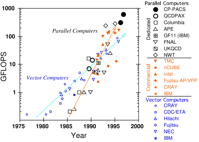
Fig. 1: Speed of dedicated computers developed by lattice physicists, together with those of recent commercial machines.

When we try to perform a numerical evaluation of the euclidian path integral (2.3), we quickly encounter the following two difficulties: First, the dimension of integration is huge. Even on a quite small lattice, for example, $10^{4}$, a 10 000 dimensional integration is required for each degrees of freedom. Second, the integrand drastically changes its magnitude, forming a quite sharp peak in configuration space. This is caused by the factor $e^{-S}$ in (2.3). The peaks correspond to the classical solutions and the width of the peaks the quantum fluctuations. Therefore, a naive mesh method to evaluate an integral cannot give a reliable value until the mesh becomes extremely fine. These difficulties can be solved by introducing the Monte Carlo method: In order to evaluate the integral, we generate the sample points with a probability proportional to $e^{-S}$, in place of the mesh points in the naive method. In the text books, we can find several techniques to generate sample points with the correct weight; the heat-bath method, the Metropolis method, the Langevin method, etc. The number of sample points required for a given accuracy is much smaller than that required in the mesh method, and has no strong dependence on the dimension of the integration.

Nevertheless, when we want to obtain a precise result, which is indispensable in phenomenological studies, the required computer power is enormous. In order to perform a reliable extrapolation of physical quantities to the continuum limit by suppressing lattice artifacts, the lattice should be fine enough while keeping a sufficiently big physical volume. Simultaneously, we need a high statistical accuracy which requires a large number of sampling points.

In order to generate a configuration (a sample point) in the SU(3) pure gauge theory, the conventional pseudo heat-bath method[14] requires about 5 700 floating point operations per link. Vector computers in the ’80s and parallel computers in the ’90s have supported the development of numerical simulations in lattice QCD. As one of the largest user groups in high performance computing, lattice physicists have also contributed a lot to the development of computer technology itself. Several groups of lattice physicists have even developed parallel computers dedicated to lattice QCD[15, 16, 17]. Fig. 1 shows the speed of recent dedicated machines for lattice QCD. On the CP-PACS constructed at the University of Tsukuba[17], more than 10 000 configurations on a $64^{3}\times 112$ lattice can be generated in a day.

When the system includes dynamical fermions, different algorithms had to be developed as we cannot have Grassmann variables directly on the computers. However, even with the latest algorithm[18, 19], several hundred times more computer time is required for fermions. Therefore, major QCD simulations on large lattices have been performed in the approximation that dynamical pair creation/annihilation of quarks are neglected (quenched QCD). Realistic simulations of QCD with dynamical quarks (full QCD) have just begun on recent high performance computers, by combining big computer power with the idea of improved lattice actions which shall be discussed in Sec. 3.

3 Improved lattice actions

3.1 From BETTER to MUST

In the scaling region near the continuum limit, we expect that the lattice results reproduce the continuum results at distances larger than about the correlation length. However, in general, expectation values at short distances in lattice units deviate from the continuum results even at large $\beta$. Therefore, in order to extract a prediction for the continuum limit, precise data at large distances on a correspondingly large lattice are required. Such simulations are quite expensive, in particular, near the continuum limit.

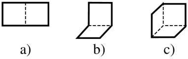
Fig. 2: Loops of length 6; (a) rectangle, (b) chair, and (c) parallelogram.

On the other hand, due to the universality, there are infinitely many candidates for the lattice action describing the same continuum limit, i.e. we can introduce additional terms to the standard action without affecting the continuum limit. For example, the lattice gauge action may contain non-minimal loops besides the plaquettes adopted in the standard action: Using loops up to length 6, we can write

$$S_{gauge}=-\beta\left\{c_{0}\sum P_{\rm plaq}+c_{1}\sum P_{\rm rect}+c_{2}\sum P_{\rm chair}+c_{3}\sum P_{\rm para}\right\},$$ (3.1)

where $P_{\rm rect}$, $P_{\rm chair}$, and $P_{\rm para}$ are rectangle, chair, and parallelogram loops shown in Fig. 2. The coefficients in (3.1) should satisfy a relation $c_{0}+8c_{1}+16c_{2}+8c_{3}=1$ in order to obtain the conventional continuum gauge action in the limit $a\rightarrow 0$ with the identification (2.10). Hence, three parameters are left free. From the universality, the long distance behavior of the theory is insensitive to these additional parameters. However, short distance properties do depend on these parameters. Therefore, a judicious choice of the additional parameters may suppress the short distance lattice artifacts even at moderate values of the lattice spacing. Such actions are called “improved actions”.

Recently, much progress has been reported in improving lattice actions[20, 21]. When an appropriate improved action is obtained, we will be able to perform a reliable extrapolation to the continuum limit using data obtained on coarse lattices. It is, of course, better to apply such an action to save money on computer time. However, through recent developments in numerical studies of lattice QCD, we now have stronger motivations to improve the action.

As the first motivation, we would like to introduce the recent results of high statistic simulation in quenched QCD by the CP-PACS Collaboration[9]. The quenched light hadron spectrum is computed for Wilson quarks on lattices with the spatial size $\approx 3$fm to an accuracy of 1–3% in the continuum limit. The baryon spectrum turns out to show a systematic disagreement which is of the order 10% (maximally 10 standard deviations) from the experimental values, which is considered as evidence of systematic errors due to the quenching approximation. Therefore, in order to test QCD to an accuracy better than $O(10\%)$, we have to perform full QCD simulations without the quenching approximation. Full QCD simulations are, however, extremely computer time consuming compared to those of quenched QCD. Even with the TFLOPS-class computers that are becoming available, high statistics studies, indispensable for reliable results, will be difficult for lattice sizes exceeding $32^{3}\times 64$. Since a physical lattice size of $L\approx 2.5$–3.0fm is needed to avoid finite-size effects, the smallest lattice spacing one can reasonably reach will be $a\sim 0.1$fm. Hence lattice discretization errors have to be controlled with simulations carried out at lattice spacings larger than this value. This will be a difficult task with the standard plaquette and Wilson quark actions since discretization errors are of order 20–30% even at $a\approx 0.1$fm.

We also encounter difficulties with the standard action in a study of finite temperature QCD. In the simulation of a finite temperature system, the spatial lattice size should be sufficiently large in order to approximately realize the thermodynamic limit. With the limitation of the computer power, this means that we have to suppress the lattice size in the time direction $N_{t}$. Currently $N_{t}\approx 4$–6 is used in most simulations with dynamical quarks. Because the temperature is given by $T=1/N_{t}a$, the corresponding lattices are coarse; for $T\sim T_{c}\approx 100$–200MeV, $a\sim 0.2$–0.4fm. Subsequent lattice artifacts sometimes make the analysis and interpretation of lattice results not a straightforward task.

The basic idea behind improvement may be obtained by considering the lattice derivative. The naive derivative $\mathchar 28929\relax_{x}f(x)={1\over{2a}}[f(x+a)-f(x-a)]$ converges to the continuum derivative with errors of $O(a^{2})$. We can reduce this error down to $O(a^{4})$ by replacing $\mathchar 28929\relax_{x}\rightarrow\mathchar 28929\relax_{x}-{a^{2}\over 6}\mathchar 28929\relax_{x}^{3}$ which operates on fields at up to next nearest neighbor sites. Similar substitution is effective also to obtain a lattice action that approaches to the continuum action much smoothly. Here, however, what we want to obtain is not a smoother lattice action, but an action which leads to smaller discretization errors in the physical observables (2.3) containing all the quantum corrections.

Several different strategies have been proposed to obtain such a lattice action. Two major approaches are the renormalization group (RG) improvement programs first proposed by K.G. Wilson[22], and the perturbative improvement programs started by K. Symanzik[23]. In the following subsections, I describe these methods in more detail. Irrespective to the differences in approach, the final goal of improvement is to obtain a lattice action which shows scaling from a coarser lattice.

In general, improved lattice actions contain additional terms (interactions that usually have a wider spatial size) compared with the standard action. Because such additional terms make the simulation quickly difficult and computer time consuming, the efficiency of improvement should be tested for each of the new terms introduced.

3.2 Symanzik improvement

In Symanzik’s method, we improve physical quantities using a result of perturbative computations[23, 24]. It consists of the following procedures:

  (i)

Compute a set of physical quantities in perturbation theory using a lattice action with non-minimal interactions.

  (ii)

Adjust the non-minimal coupling parameters to remove the leading finite $a$ deviations from the continuum limit in these physical quantities.

A conventional choice for the physical quantities in this program are the low-dimensional operators in the effective action. When discretization errors are eliminated up to the $n$th order in $a$, the resulting action is said to be “$O({a^{n}})$ improved”. For example, the standard plaquette gauge action has $O(a^{2})$ errors. Several different actions removing these errors, to tree or one-loop level, have been proposed depending on the choice of additional terms[25, 26, 27].

This improvement program is quite attractive because an improved action can be obtained by an analytic calculation. Nevertheless, the method in its naive form remained unsuccessful for a long time. The reason is that the perturbation theory, using the bare gauge coupling constant as the expansion parameter, has poor convergence, and the perturbative results do not agree with the results from numerical simulations which are mostly performed at $\beta=O(1)$.

The failure of the bare perturbation theory may be understood as follows. The bare perturbation theory is based on an expansion of the link variable (2.7)

$$U_{x,\mu}\approx 1+igaA_{\mu}(x)-\frac{1}{2}\,g^{2}a^{2}\,A_{\mu}(x)^{2}+\,\cdots.$$ (3.2)

In order that the perturbation theory works well, the higher order terms in (3.2) should be much smaller than 1. However, in actual simulations, the link variable deviates much from unity; we obtain the plaquette expectation value about 0.4–0.6. Perturbatively, this deviation is caused by large contributions of “tadpole” diagrams[28]: By fixing the gauge appropriately, the mean value of the link variable can be expressed as

$$u_{0}=\langle U_{x,\mu}\rangle\approx 1-\frac{1}{2}\,g^{2}a^{2}\,\langle A_{\mu}(x)^{2}\rangle+\,\cdots.$$ (3.3)

Because of a quadratic divergence in the tadpole contribution $\langle A_{\mu}(x)^{2}\rangle$, higher order terms $[g^{2}a^{2}\langle A_{\mu}(x)^{2}\rangle]^{k}$ are suppressed only by $g^{2k}$, instead of the naive factor $g^{2k}a^{2k}$. In the simulations, $g^{2}\sim O(1)$.

3.2.1 Mean-field improvement

The convergence of the perturbation theory can be improved by an appropriate choice of the expansion parameter. Recent significant progress in Symanzik improvement is based on a combination of the Symanzik improvement program with an idea of “mean-field improvement (tadpole improvement)” of the perturbation theory[29, 28]: Consider a modified expansion of the link variable around the mean-field value $u_{0}$:

$$U_{x,\mu}=u_{0}\exp\left[ig_{\rm MF}\,aA^{\prime}_{\mu}(x)\right].$$ (3.4)

With much smaller quantum fluctuations, we will obtain a much better converging perturbation theory with $A^{\prime}_{\mu}(x)$. From a substitution

$$S_{\rm gauge}=-\beta\sum_{\rm plaq}P_{\rm plaq}\;\;\longrightarrow\;\;-u_{0}^{4}\,\beta\sum_{\rm plaq}\frac{1}{u_{0}^{4}}\,P_{\rm plaq},$$ (3.5)

we find $g_{\rm MF}=g/u_{0}^{2}$. A conventional choice for $u_{0}$ is $u_{0}=\langle P\rangle^{1/4}$. The perturbation theory using $g_{\rm MF}$ as the expansion parameter is shown to agree with numerical results much more precisely even at the large bare coupling $g$ used in numerical simulations[28, 21].

Therefore, a prescription for a mean-field improved Symanzik improvement is to introduce a third step:

  (iii)

Multiply an appropriate power of $u_{0}$ to the perturbatively determined coefficients of the Symanzik action.

It is, however, not trivial whether the non-perturbative quantities we are interested in are also sufficiently improved by this method. Non-perturbative tests are required to confirm the efficiency.

3.2.2 Symanzik-improved Wilson quark action

The Wilson quark action has $O(a)$ errors. Symanzik-improved Wilson quark action was studied by Sheikholeslami and Wohlert[30]. The $O(a)$ improved action reads

$$S_{\rm clover}=S_{\rm Wilson}+\sum_{x,\mu,\nu}\frac{i}{2}\,c_{\rm SW}K\,\overline{\psi}_{x}\sigma_{\mu,\nu}F_{x,\mu\nu}\psi_{x},$$ (3.6)

where $\sigma_{\mu,\nu}=\frac{1}{2}[\gamma_{\mu},\gamma_{\nu}]$. Here $F_{x,\mu\nu}$ is the field strength on lattice. Because we conventionally construct $F_{x,\mu\nu}$ in terms of four plaquette-like loops in the $\mu\nu$ plane around the site $x$, the action (3.6) is called the “clover action”.

The coefficient $c_{\rm SW}$, the clover coefficient, is 1 at the tree-level. Its mean-field improvement can be done by $c_{\rm SW}\rightarrow c_{\rm SW}/u_{0}^{3}$ because the field strength gives the factor $u_{0}^{-4}$ while the hopping parameter is redefined as $K\rightarrow K/u_{0}$[28, 31].

3.2.3 Non-perturbative determination of a Symanzik action

Recently an approach to combine the Symanzik method with a non-perturbative study was proposed:

  (i^′)

Measure a set of physical quantities by a numerical simulation using a perturbatively inspired form of the Symanzik action, varying the coupling parameters freely.

  (ii^′)

Adjust the non-minimal coupling parameters of the action such that several physical requirements are satisfied by the numerical data.

An attempt to determine $c_{\rm SW}$ non-perturbatively requiring a PCAC relation to hold is reported in Ref. ?. A technical background for this is the development of the Schrödinger functional method in which the lattice correction to the PCAC relation is sensitive to the value of $c_{\rm SW}$.

3.3 RG improvement

In order to see the basic idea of RG improvement[22], let us consider, as a typical example, a block transformation of scale factor 2. A correlation function $G_{\rm block}(r)$ on the blocked lattice is related to the corresponding correlation function $G_{\rm orig}(r)$ on the original lattice by $G_{\rm block}(r)\approx G_{\rm orig}(2r)$, where the distance $r$ is measured in lattice units. Therefore, when we have the continuum behavior at distances $r\mathop{\vtop{\halign{#\cr$\hfil\displaystyle{>}\hfil$\crcr\kern 0.5pt\nointerlineskip\cr$\sim$\crcr\kern 0.5pt\cr}}}\limits r_{0}$ on the original lattice, then the continuum behavior is realized at $r_{0}/2$ on the blocked lattice. This means that a block transformation improves the action.

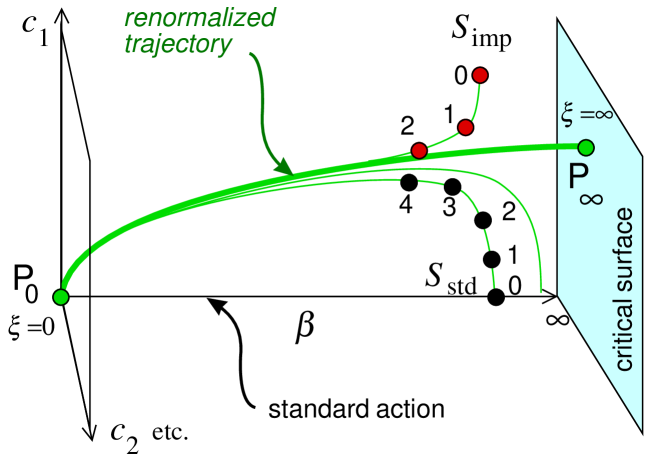
Fig. 3: RG flow and the renormalized trajectory in the SU(3) gauge theory.

A block transformation generally induces many effective interactions in the effective action:

$$\exp\left\{-S_{\rm block}[\phi_{\rm block}]\right\}=\int[{\rm d}\phi_{\rm orig}]\,K[\phi_{\rm block},\phi_{\rm orig}]\,\exp\left\{-S_{\rm orig}(\phi_{\rm orig})\right\},$$ (3.7)

where the kernel $K[\phi_{\rm block},\phi_{\rm orig}]$ defines the block transformation $\phi_{\rm orig}\rightarrow\phi_{\rm block}$. Therefore, repeated applications of a block transformation defines a flow (RG flow) in the infinite dimensional coupling parameter space of effective actions.

For the SU(3) gauge theory, we imagine the RG flows to be as shown in Fig. 3. In this figure, $c_{1}$, $c_{2}$, etc. denote additional coupling parameters [cf. the action (3.1)]. The points on the $\beta$ axis correspond to the standard one plaquette action at various $\beta$. Because a block transformation makes the correlation $\xi$ in lattice units smaller, RG flows are oriented towards smaller $\beta$. The hyperplane at $\beta=\infty$ ($\xi=\infty$) is called the critical surface. When the starting action $S^{(0)}$ is in the scaling region that is close to the critical surface, we expect that all trajectory flows first along the critical surface, and then leaves the critical surface to gradually approach to a universal curve, the “renormalized trajectory” (RT), after sufficiently many steps, because the long distance physics is universal in the scaling region. The number of block transformations required to get sufficiently close to RT is nothing but $\log_{2}$ of the minimum distance to obtain continuum behavior with $S^{(0)}$.

We expect that the RT is also a RG flow starting from an infra-red fixed point, $P_{\infty}$, on the critical surface. Because the RT is directly connected to the action $P_{\infty}$ in the continuum limit by block transformations, actions on the RT show continuum properties from the shortest distances on the lattice. Therefore, the actions on the RT are called “perfect actions”[33].

If an infinite number of coupling parameters are admitted, a perfect action is a goal of improvement. In reality, we can not handle infinitely many couplings. A few approaches are proposed to obtain an improved action in a finite dimensional subspace of the coupling parameters.

3.3.1 Fixed point action approach

Hasenfratz and Niedermayer proposed to use an approximation of the fixed point action $P_{\infty}$ as an approximate perfect action[33]. In asymptotically free theories, because the critical surface is located in the weak coupling region, a compact integral equation for $P_{\infty}$ can be written. With a proper Ansatz for the effective action, we can numerically solve the fixed point action $P_{\infty}$. The most delicate point is the choice of the finite-dimensional Ansatz action (“parametrization”). It is noted that generally, a large number of coupling parameters are required to achieve a good approximation for $P_{\infty}$.

Many developments are reported in the literature; see Refs. ?, ? for more details. For a trial to compute the RT nonperturbatively, see Ref. ?. The fixed point action for full QCD is discussed in Refs. ?, ?, ?.

3.3.2 Iwasaki’s method

In an alternative approach, proposed in 1983 by Iwasaki[38], the practical constraint for the number of coupling parameters in numerical simulations is taken more seriously. In this approach, instead of trying to obtain an approximate perfect action directly, one attempts to accelerate the approach to the RT by taking advantage of the extended parameter space:

  (i)

We restrict ourselves to a small dimensional coupling parameter space consisting only of interactions which can be easily implemented in numerical simulations.

  (ii)

Find a set of coupling parameters that minimizes the distance to the RT after a few block transformations.

Because a block transformation induces many effective couplings, the number of coupling parameters for the initial action can be quite small.

As an illustration, let us consider an action $S_{imp}$ in the two-dimwnsional coupling parameter space $(\beta,c_{1})$ shown in Fig. 3, and suppose that the additional parameter $c_{1}$ is adjusted such that the RG flow gets sufficiently close to RT after, say, 2 block transformations. This means that, when we simulate the system using $S_{imp}$, a separation of $2^{2}a$ is enough to get the continuum properties.

Iwasaki applied this program to the SU(3) gauge theory[38]. Asymptotic freedom again helps us to compute such $S_{imp}$:

$$S_{imp}=-\beta\left\{c_{0}\sum P_{\rm plaq}+c_{1}\sum P_{\rm rect}\right\},$$ (3.8)

where $c_{0}=1-8c_{1}$ and $c_{1}=-0.331$ ($-0.293$) to minimize the distance to RT after one (two) block transformations. This action is remarkably simple. It is easy to write a vectorized and/or parallelized program for this action. Good efficiency in removing several lattice artifacts is reported by the Tsukuba group[39, 40]. An application to finite temperature QCD with dynamical quarks[41] will be discussed in Sec. 5.1.2.

4 $SU(3)$ gauge theory at finite temperature

As the first step towards finite temperature QCD, in this section, let us study the case of the SU(3) pure gauge theory, or, equivalently, QCD in the approximation that dynamical creation/annihilation of quarks are neglected (quenched QCD). Although quenched QCD is not quite realistic, we can obtain high statistics data on large lattices in this case. Therefore, it provides us with a good lesson for full QCD studies.

4.1 Deconfining transition in SU(3) gauge theory

In a study of the deconfining transition in pure gauge theories, it is useful to consider the “Polyakov loop”[42]

$$\mathchar 28938\relax_{{\vec{x}}}=\frac{1}{N_{c}}\,{\rm Tr}\left(\prod_{t=1}^{N_{t}}U_{{\vec{x}},t;4}\right).$$ (4.1)

In the path integral, $\mathchar 28938\relax_{{\vec{x}}}$ is just the factor from the current appearing when a static charge is located at the spatial point ${\vec{x}}$. Therefore, except for the renormalization corrections, $\langle\mathchar 28938\relax\rangle\sim e^{-F_{q}/T}$, where $F_{q}$ is the free energy of the static charge. We expect that $F_{q}=\infty$ (i.e. $\langle\mathchar 28938\relax\rangle=0$) when charge is confined, while $F_{q}<\infty$ ($\langle\mathchar 28938\relax\rangle>0$) when charge is deconfined. Therefore, $\langle\mathchar 28938\relax\rangle$ is an order parameter for the deconfining transition.

The global symmetry behind this order parameter is given by

$$U_{x,\mu}\rightarrow\left\{\begin{array}[]{ll}z\,U_{x,\mu}&\mbox{if $x_{4}=0$ and $\mu=4$}\\ U_{x,\mu}&\mbox{otherwise}\end{array}\right.$$ (4.4)

where $z$ is an element of the center group Z($N_{c}$) of the gauge group SU($N_{c}$). Because $z$ commutates with any element of SU($N_{c}$), the plaquettes as well as more extended closed loops are invariant under the transformation (4.4), i.e. the pure gauge actions (2.8), (3.1), etc. are invariant under (4.4). On the other hand, because $\mathchar 28938\relax_{{\vec{x}}}$ crosses the hyper plane $x_{4}=0$ only once, $\mathchar 28938\relax_{{\vec{x}}}\rightarrow z\,\mathchar 28938\relax_{{\vec{x}}}$ under (4.4). Therefore, a non-vanishing vacuum expectation value of $\mathchar 28938\relax$ implies the spontaneous breakdown of the center $Z(3)$ global symmetry at the deconfining transition.

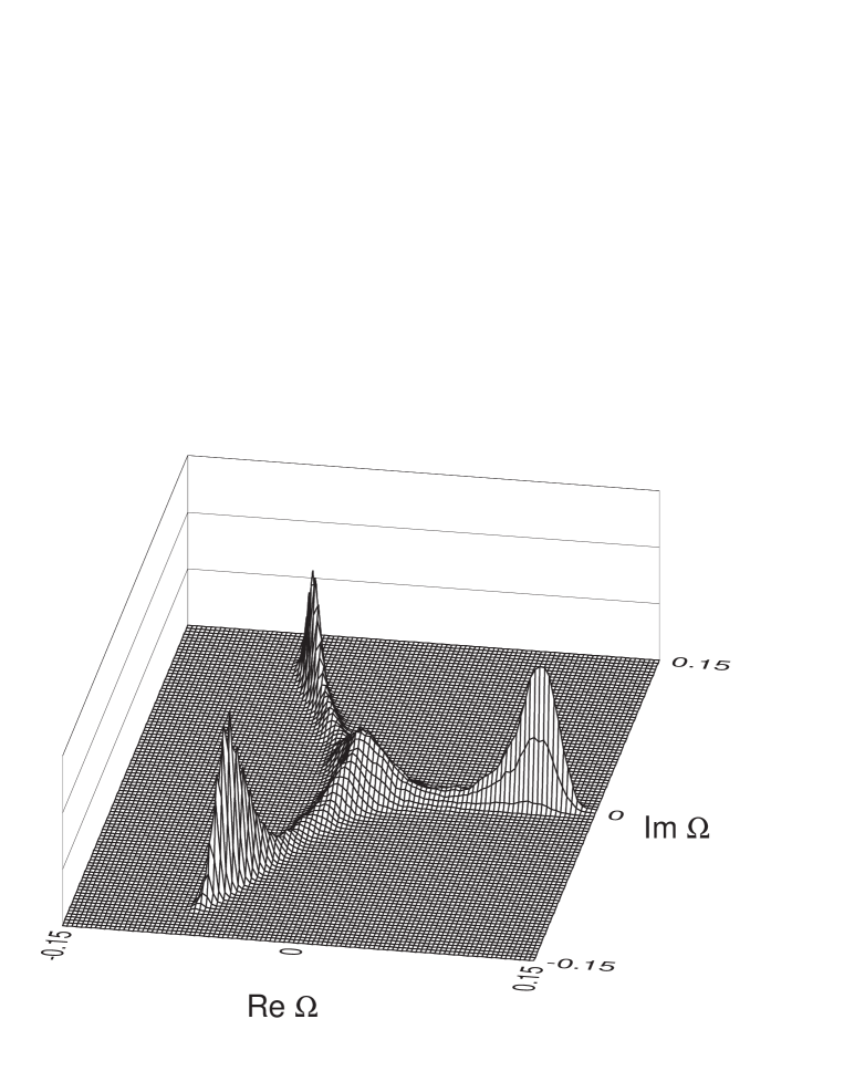
Fig. 4: Polyakov loop histogram in the SU(3) gauge theory at the deconfining transition point obtained on a $24^{2}\times 36\times 4$ lattice[44].

a) b)

Fig. 5: Polyakov loop histogram for $|\mathchar 28938\relax|$ at the deconfining transition point obtained on (a) $N_{t}=4$ and (b) 6 lattices [44]. The simulation temperature for the $24^{3}\times 6$ lattice is slightly lower than the transition temperature.

We may study the nature of the deconfining transition using an effective theory of the Polyakov loops in three dimensions. Because the order-disorder phase transition in a three dimensional Z(3) spin model (the Potts model) is first order, we may expect that the deconfining transition in the SU(3) gauge theory is also first order, when the interaction in the effective theory of $\mathchar 28938\relax_{\vec{x}}$ is short ranged[43].

Figure 4 is a result of the Polyakov loop histogram in the complex plane, obtained just at the deconfining transition temperature in the SU(3) gauge theory[44]. The peak at the center $\mathchar 28938\relax\sim 0$ is the contribution of the symmetric phase (low temperature confining phase) and the three peaks at non-zero $|\mathchar 28938\relax|$ with $\arg\mathchar 28938\relax\sim 0$ and $\pm 2\pi/3$ are from the Z(3) broken phases. Clear separation of these peaks, as well as the lattice volume dependence shown in Fig. 5, implies that the transition is of first order. The order of the transition is confirmed by a precise finite size scaling test[45, 44]. Accordingly, the short range nature of the effective interaction between the Polyakov loops is also shown[45].

4.2 Transition temperature

Precisely speaking, we have no real transition on a finite lattice. The transition point $\beta_{c}(N_{t})$ for each fixed $N_{t}$ can be computed by an extrapolation to the infinite spatial volume using a finite size scaling. The value of $\beta_{c}(N_{t})$ is translated into physical units by fixing the scale at this value of $\beta$.

In pure gauge theories, the scale is conventionally fixed with the string tension in a static quark potential $\sigma$ at zero temperature.

$$\sigma a^{2}=-\lim_{A\rightarrow\infty}\frac{1}{A}\,\ln\langle W(A)\rangle$$ (4.5)

where $W(A)=\prod_{\ell\in\partial A}U_{\ell}$ is the Wilson loop with area $A$. We then obtain $T_{c}/\sqrt{\sigma}=1/[N_{t}\sqrt{\sigma a^{2}(\beta_{c}(N_{t}))}]$. Using recent data[46] for $\sigma a^{2}$, we obtain $T_{c}/\sqrt{\sigma}\approx 0.63(1)$ in the continuum limit ($N_{t}\rightarrow\infty$) from the standard action[44, 47]. Results from various improved actions are $T_{c}/\sqrt{\sigma}\approx 0.62$–0.66 [39, 48, 49, 50]. Adopting a phenomenological value $\sigma=(427\mbox{MeV})^{2}$ from a charmoniun spectrum[51], we obtain $T_{c}\sim 270$MeV.

4.3 Thermodynamic quantities

In a phenomenological study of the quark-gluon plasma in heavy ion collisions and in the early Universe, it is important to evaluate thermodynamic quantities such as the energy density $\epsilon$ and the pressure $p$, near the transition temperature of the deconfining phase transition. These quantities are defined by derivatives of the partition function with respect to the temperature $T$ and the physical volume $V$ of the system

$$\epsilon=-\frac{1}{V}\,\frac{\partial\ln Z}{\partial T^{-1}},\hskip 22.76219ptp=T\,\frac{\partial\ln Z}{\partial V}.$$ (4.6)

On a lattice with the size $N_{s}^{3}\times N_{t}$, $V$ and $T$ are given by $V=(N_{s}a_{s})^{3}$ and $T=1/(N_{t}a_{t})$, with $a_{s}$ and $a_{t}$ the lattice spacings in spatial and temporal directions. Because $N_{s}$ and $N_{t}$ are discrete parameters, the partial differentiations in (4.6) are performed by varying $a_{s}$ and $a_{t}$ independently.

Anisotropy on the lattice is introduced by different coupling parameters in temporal and spatial directions. For an SU($N_{c}$) gauge theory, the standard plaquette action on an anisotropic lattice is given by

$$S=-\beta_{s}\sum_{x,\,i<j\neq 4}P_{x,ij}-\beta_{t}\sum_{x,\,i\neq 4}P_{x,i4},$$ (4.7)

where $P_{x,\mu\nu}$ is defined by (2.9). Then the energy density and pressure, renormalized at $T=0$, are given by[52, 53]

$$\epsilon a_{s}^{4} = 3\xi^{2}\left\{\frac{\partial\beta_{s}}{\partial\xi}\,\left(\langle P_{s}\rangle-\langle P\rangle_{0}\right)+\frac{\partial\beta_{t}}{\partial\xi}\,\left(\langle P_{t}\rangle-\langle P\rangle_{0}\right)\right\}$$ (4.8)

$$pa_{s}^{4} = \xi^{2}\left\{\left(\frac{\partial\beta_{s}}{\partial\xi}+\frac{a_{s}}{\xi}\frac{\partial\beta_{s}}{\partial a_{s}}\right)\,\left(\langle P_{s}\rangle-\langle P\rangle_{0}\right)\right.$$ (4.9)

$$\left.+\left(\frac{\partial\beta_{t}}{\partial\xi}+\frac{a_{s}}{\xi}\frac{\partial\beta_{t}}{\partial a_{s}}\right)\,\left(\langle P_{t}\rangle-\langle P\rangle_{0}\right)\right\},$$

where $\langle P_{s(t)}\rangle$ is the space(time)-like plaquette expectation value and $\langle P\rangle_{0}$ the plaquette expectation value at the same coupling parameters on a zero-temperature lattice. In these expressions, the variables $\xi\equiv a_{s}/a_{t}$ and $a_{s}$ are chosen to control the lattice spacings.

Therefore, in order to compute $\epsilon$ and $p$ from the results of simulations, the values for the derivatives of gauge coupling constants with respect to the anisotropic lattice spacings (the anisotropy coefficients) are required.

The calculation of these anisotropy coefficients in the lowest order perturbation theory was done by Karsch[53]. [Coefficients needed for the case with dynamical quarks are also computed perturbatively in Ref. ?.] However, the bare perturbation theory is not reliable for the values of $\beta$ where MC simulations are performed. Accordingly, the perturbative coefficients are known to lead to a pathological result of negative pressure at strong couplings used in the numerical simulations. In the case of SU(3) gauge theory, the transition is of first order. At a first order transition point, we have a finite gap for the energy density, the latent heat, but expect no gap for the pressure. It is known that the perturbative anisotropy coefficients have the problem of non-vanishing pressure gap at the deconfining transition point: $\mathchar 28929\relax p/T^{4}=-0.32(3)$ and $-0.14(2)$ on $24^{2}\times 36\times 4$ and $36^{2}\times 48\times 6$ lattices[44]. Therefore, we need non-perturbative values for the anisotropy coefficients.

We are mainly interested in the values of the anisotropy coefficients for the case of isotropic lattices ($\beta_{s}=\beta_{t}\equiv\beta$, i.e. $\xi=1$) because most simulations are performed in this case. At $\xi=1$, we have $\left(a_{s}\partial\beta_{s}/\partial a_{s}\right)_{\xi=1}=\left(a_{s}\partial\beta_{t}/\partial a_{s}\right)_{\xi=1}=a{\rm d}\beta/{\rm d}a$, where $a{\rm d}\beta/{\rm d}a$ is the beta-function. Furthermore, a combination of the remaining two anisotropy coefficients is known to be related to the beta-function[53]: $\left(\partial\beta_{s}/\partial\xi\right)_{\xi=1}+\left(\partial\beta_{t}/\partial\xi\right)_{\xi=1}=-(1/2)\,a{\rm d}\beta/{\rm d}a.$ Therefore, we need to estimate nonperturbative values of the beta-function $a{\rm d}\beta/{\rm d}a$ and one independent combination of the anisotropy coefficients.

In connection to this, it is useful to consider a combination $\epsilon-3p$ which is defined via a uniform scale transformation:

$$\epsilon-3p = -\frac{a^{4}}{V/T}\left(\frac{1}{T}\frac{\partial}{\partial(1/T)}+3V\frac{\partial}{\partial V}\right)\ln Z=-\frac{a^{4}}{V/T}\left(a_{t}\frac{\partial}{\partial a_{t}}+a_{s}\frac{\partial}{\partial a_{s}}\right)\ln Z$$ (4.10)

$$= -3T^{4}N_{t}^{4}\,a\frac{{\rm d}\beta}{{\rm d}a}\left(\langle P_{s}+P_{t}\rangle-2\langle P\rangle_{0}\right)$$

at $\xi=1$. Therefore, this combination depends only on the beta-function $a{\rm d}\beta/{\rm d}a$. Several non-perturbative values for the beta-function are available; from a MC renormalization group study[55], from a study of the transition temperature[47], or from the $\beta$-dependence of a physical quantity, such as the string tension[46].

a)

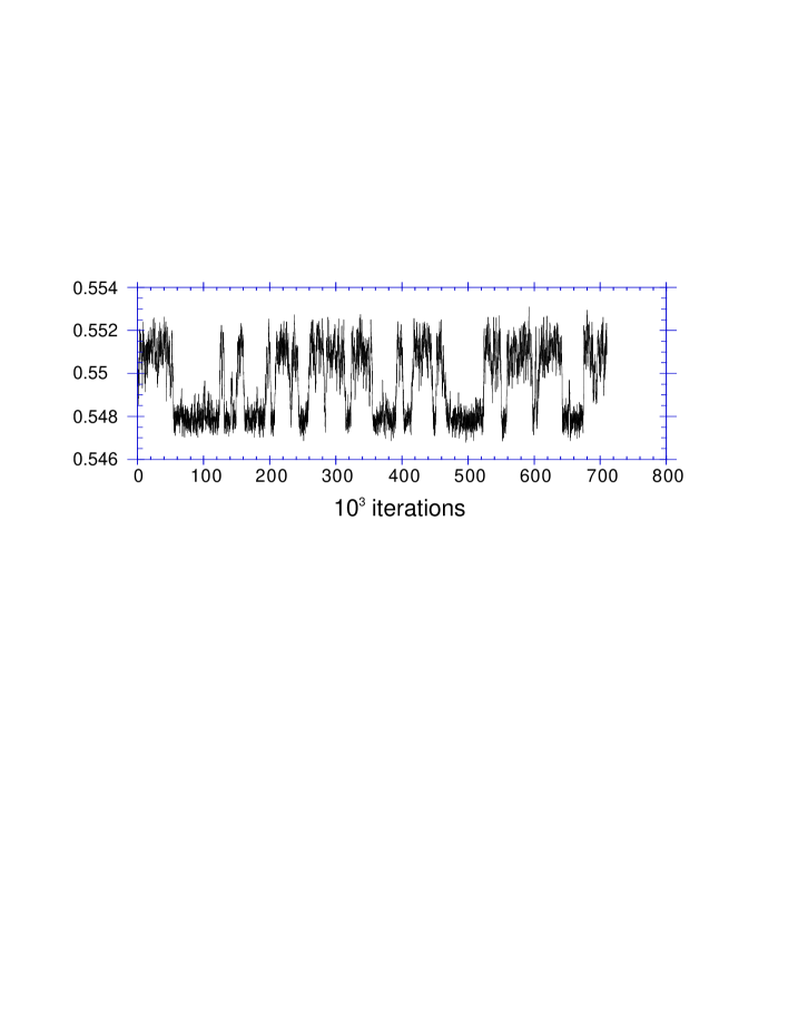
b)

Fig. 6: Plaquette history in the SU(3) gauge theory at the deconfining transition point obtained on (a) $24^{2}\times 36\times 4$ and (b) $36^{2}\times 48\times 6$ lattices[44].

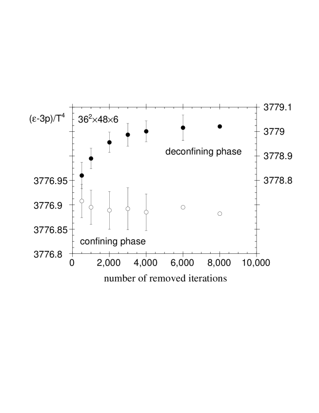
Fig. 7: $(\epsilon-3p)/T^{4}$ average in each of the confining and deconfining phases in the SU(3) gauge theory at the deconfining transition point obtained on a $36^{2}\times 48\times 6$ lattice[44], as a function of the removed iterations around the phase flip-flops shown in Fig. 6(b). $\epsilon-3p$ is defined by (4.10) using the perturbative beta-function.

As an application, we compute the energy gap $\mathchar 28929\relax\epsilon$, identified with $\mathchar 28929\relax(\epsilon-3p)$ because we expect $\mathchar 28929\relax p=0$, at the deconfining transition in the SU(3) gauge theory. In order to determine the expectation values in each phase, we first inspect the “flip-flops” between the confining and deconfining phases in Monte Carlo time histories (see Fig. 6 for example), and separate the runs into the two phases by the flip-flops. A sufficient number of iterations around the flip-flops and around the spikes should be removed to avoid contamination from transition stages. Fig. 7 shows an example of expectation values of observables in each phase as a function of the number of removed iterations. We can obtain stable results when a sufficiently large number of iterations from the transition stages are removed. Note that such unambiguous separation of two phases is possible only on large lattices where the persistence time of each phase is sufficiently long. Using the beta-function calculated from recent string tension data[46], we find that $\mathchar 28929\relax(\epsilon-3p)/T_{c}^{4}=2.072(43)$ and 1.578(42) for $N_{t}=4$ and 6, respectively, with the standard action[44]. Using Symanzik improved actions with $2\times 1$ loops, values of 1.57(12) and 1.40(9) are reported for tree-level and tadpole-improved actions on a $32^{3}\times 4$ lattice[56]. More data at larger $N_{t}$ are needed to make a reliable continuum extrapolation.

In order to determine $\epsilon$ and $p$ separately, we need one more input as discussed above. A non-perturbative determination of a combination of the anisotropy coefficients was attempted in Refs. ?, ?, ?, ? using a matching of space-like and time-like Wilson loops on anisotropic lattices (the matching method)[57]. Alternatively, we can evaluate a non-perturbative value of pressure directly from the Monte Carlo data by the integral method[61]: assuming homogeneity of the system, expected for the case of large spatial volume, we obtain the relation $p=-f$, where $f$ is the free energy density, $f=-\frac{T}{V}\ln Z$. For the case of pure gauge theory with the plaquette action, $f$ can be evaluated by integrating the plaquette $\langle P\rangle$ in term of $\beta$ on isotropic lattices, since $\frac{\partial}{\partial\beta}\ln Z=6N_{s}^{3}N_{t}\langle P\rangle$. The resulting value of the pressure, in turn, provides us with a non-perturbative estimate of a combination of the anisotropy coefficients[47, 61, 62, 63]. Recently, a new method, using a measurement of the finite temperature deconfining transition curve in the lattice coupling parameter space extended to anisotropic lattices, was proposed[64].

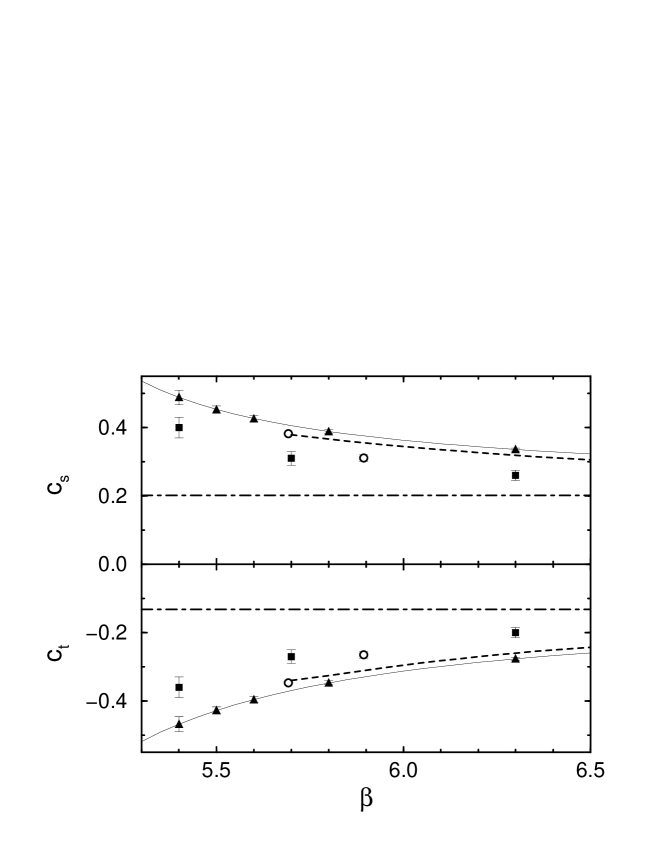
Fig. 8: Anisotropy coefficients (Karsch coefficients) in the SU(3) gauge theory. Dot-dashed lines are the results of the perturbation theory [53]. Filled squares are the results of a matching method obtained in Ref. ?. Filled triangles and thin lines are the results of a matching method [60] combined with the beta-function using a recent string tension data[46]. Dashed lines are the results of the integral method [47]. Open circles are the results of a new method using the transition curve in the coupling parameter space for anisotropic lattices [64].

Recent results for the anisotropy coefficients in the form

$$c_{s}=\left(\frac{\partial g_{s}^{-2}}{\partial\xi}\right)_{a_{s}:{\rm fixed},\,\xi=1},\hskip 22.76219ptc_{t}=\left(\frac{\partial g_{t}^{-2}}{\partial\xi}\right)_{a_{s}:{\rm fixed},\,\xi=1},$$ (4.11)

(Karsch coefficients) with $\beta_{s}=2N_{c}g_{s}^{-2}\xi^{-1}$ and $\beta_{t}=2N_{c}g_{t}^{-2}\xi$, are summarized in Fig. 8. Applying these results, we can reanalyze the pressure gap. At the deconfining transition point for $N_{t}=6$, we find $\mathchar 28929\relax p/T^{4}=-0.003(17)$ using the results of Ref. ? or $-0.040(43)$ using the result of Ref. ?. We find that the problem of a non-vanishing pressure gap is removed with non-perturbative anisotropy coefficients.

4.4 Interface tension

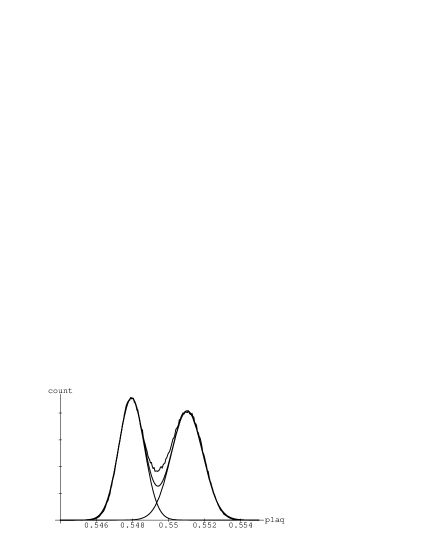
a) b)

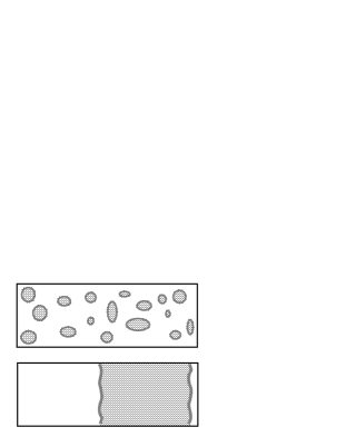
Fig. 9: (a) Plaquette histogram in the SU(3) gauge theory at the deconfining transition point obtained on a $24^{2}\times 36\times 4$ lattices[44]. See Fig. 6(a) for the corresponding time history. The two peaks are separately fitted with two Gaussian distributions. (b) Mix configurations at a first order transition point. Above: naive configuration with bubbles. Below: dominant configuration for two phase coexistence on a finite box with periodic boundary conditions.

Table I: Interface tension $\sigma_{I}/T_{c}^{3}$ computed using the histogram method for the data of $|\mathchar 28938\relax|$. Large spatial volume limit is taken, except for the results at $N_{t}=3$ where the spatial lattice volume is $12^{3}$.

$N_{t}$	standard	Symanzik action[56]		fixed point
	action[66]	tree-level	MF improved	action[68]
2	0.092(4)[67]
3		0.2434(24)	0.0158(11)	0.0307(8)
4	0.0295(21)	0.0152(26)	0.0152(20)	0.026(5)
6	0.0218(33)

Because the deconfining transition is first order for SU(3), we expect that hot and cold phases can coexist just at the transition temperature. When the transition is also of first order in full QCD, the value of the surface tension for the interface between two phases is important in a study of hadronic bubble formation in the cooling process of the quark gluon plasma at the early Universe, heavy ion collisions etc.. To gain experience for the study in full QCD, the interface tension has been measured in quenched QCD using various actions.

Recent numerical computations of the interface tension are based on the “histogram method”[65]: As shown in Fig. 6, the Monte Carlo time history of an observable that is sensitive to the transition shows flip-flops between two phases at the transition point. Accordingly, when we plot a histogram from the history, we obtain two peaks corresponding to the two phases, when the lattice size is sufficiently large. As shown in Fig. 9(a) for the case of the plaquette on a $24^{2}\times 36\times 4$ lattice, the valley between the two peaks is in general higher than that expected from an overlap of two distributions corresponding to the two peaks. This excess is due to the contribution of transition stages (mixed states) around the flip-flops discussed in Sec. 4.3. Naively, a mixed state would look like bubbles of one phase floating in the sea of another phase. With positive interface tension, however, the dominant contribution will be the configurations with minimum interface area. See Fig. 9(b). Then, because the interface area is approximately fixed from the lattice geometry, we can calculate the probability to have such a mixed state as a function of the interface tension. Comparing the result with the measured probability obtained from the histogram, we can compute the value of the interface tension[65].

The actual procedure in lattice QCD is much more complicated. We perform a finite size scaling analysis taking into account various corrections including those from capillary wave excitations on the interface[66]. Recent results from various actions are summarized in Table I. A naive continuum extrapolation using the data for $N_{t}=4$ and 6 from the standard action gives $\sigma_{I}/T_{c}^{3}=0.16(4)$, which is close to the values obtained with Symanzik improved actions at $N_{t}=4$[56], but slightly smaller than the value from a fixed point action[68].

5 Finite temperature QCD with dynamical quarks

Finally, let us study finite temperature QCD with dynamical quarks. As discussed in Sec. 2.6, a full QCD simulation requires several hundred times more computational time compared with a quenched simulation to achieve corresponding accuracy. Therefore, in many cases, results for full QCD are not yet quite quantitative.

In this lecture, we concentrate on the topics of the order of the finite temperature transition in full QCD. With dynamical quarks, the center Z($N_{c}$) transformation (4.4) is no longer a symmetry of the action. Therefore, although the Polyakov loop is still a good “indicator” of the deconfining transition (it sensitively changes its magnitude at the transition point), the group Z($N_{c}$) is no longer a good guide to study the nature of the QCD transition.

On the other hand, when quarks are light, we expect that the chiral symmetry, which is spontaneously broken in low temperatures, is recovered when the temperature is sufficiently large. Using the universality hypothesis, the nature of the finite temperature QCD transition near the chiral limit can be studied by a Ginzburg-Landau effective theory respecting the chiral symmetry of QCD, the effective $\sigma$ model. From a study of the effective $\sigma$ model at finite temperatures[69], the transition in the chiral limit (the chiral transition) is predicted to depend quite sensitively on the number of light quark flavors $N_{F}$. Let us consider QCD with $N_{F}$ degenerate light quarks. For $N_{F}\geq 3$, a first order transition is predicted from the sigma model. For $N_{F}=2$, on the other hand, the order of the transition is not quite definite in the effective $\sigma$ model; a first order transition is predicted when the anomalous axial U$\!{}_{A}$(1) symmetry is effectively restored at the transition temperature, while a second order transition is expected otherwise. However, because the U$\!{}_{A}$(1) breaking operator is a relevant operator whose coefficient grows towards the IR limit under a renormalization group transformation, the transition is more likely to be second order[71]. A non-perturbative study is required to determine the order of the transition for $N_{F}=2$ conclusively.

In nature, we know six flavors of quarks; u, d, s, c, b, and t. The lightest two quarks, u and d, are much lighter than the relevant energy scale for thermal processes near the critical temperature $T_{c}\simeq 100$–200 MeV: $m_{u}$, $m_{d}\ll T_{c}$. On the other hand, the last three quarks, c, b, and t, are sufficiently heavy that they are expected to play no appreciable roles in thermal processes near $T_{c}$. In the following, the case $N_{F}=2$ corresponds to the case where the third quark s is much heavier than the relevant energy scale; $m_{s}\gg T_{c}$, while the case $N_{F}\geq 3$ corresponds to the case $m_{s}\ll T_{c}$. Because $m_{s}\simeq 150$–200 MeV is just of the same order of magnitude as the expected values of $T_{c}$, in order to make a reliable prediction for the real world, we have to fine-tune the value of $m_{s}$ in the more realistic case of two light quarks and one heavy quark ($N_{F}=2+1$).

5.1 Chiral transition for $N_{F}=2$ QCD

Understanding the nature of the QCD transition for $N_{F}=2$ is an important step toward the clarification of the transition in the real world. When the transition in the chiral limit (the chiral transition) is second order, we expect that the transition turns into an analytic crossover at non-zero $m_{q}$, while when the chiral transition is first order, it will remain to be first order for small $m_{q}$. In order to confirm the expected crossover numerically, we have to study the lattice size dependence to see if the formation of a singularity (e.g. the increase of the peak height of a susceptibility with increasing the lattice volume) stops on sufficiently large lattices. However, it is difficult to numerically distinguish between a very weak first order transition and a crossover, especially at small $m_{q}$.

Here, the universality provides us with useful scaling relations that can be confronted with numerical results of QCD, in order to test the nature of the transition: It is plausible from an effective $\sigma$ model that, when the chiral transition is of second order, QCD with two flavors belongs to the same universality class as the three dimensional O(4) Heisenberg model[69]. The O(4) model is much simpler than the $\sigma$ model, and its scaling properties are well studied. For example, at small external field $h$ near the critical temperature $T_{c}$ for $h=0$, the pseudo-critical temperature $T_{pc}(h)$ and the peak height of the magnetic and thermal susceptibilities follow $T_{pc}-T_{c}\sim h^{z_{g}}$, $\chi_{m}^{\rm max}\sim h^{-z_{m}}$, and $\chi_{t}^{\rm max}\sim h^{-z_{t}}$, where $z_{g}=1/\beta\delta$, $z_{m}=1-1/\delta$, and $z_{t}=(1-\beta)/\beta\delta$ in terms of the O(4) critical exponents $\beta$ and $\delta$. Here the values of $\beta$ and $\delta$ for the O(4) model are well established[72]. In QCD, we identify $T\sim 6/g^{2}$, $h\sim m_{q}$, and $M\sim\langle\bar{\mathchar 28937\relax}\mathchar 28937\relax\rangle$.

In lattice QCD, an additional complication should be noted because no known lattice fermions have the full chiral symmetry on finite lattices, as discussed in Sec. 2. In particular, on a coarse lattice used in a finite temperature simulation, we sometimes encounter sizable deviations from the scaling behavior expected in the continuum limit. Therefore, the appearance of the O(4) scaling is also a useful touchstone to test the recovery of the chiral symmetry on the lattice when the chiral transition is of second order.

5.1.1 Results with staggered quarks

The O(4) scaling was first tested on the lattice for staggered quarks by the Bielefeld group[73]. Based on simulations on an $8^{3}\times 4$ lattice at $m_{q}a=0.02$, 0.0375, and 0.075 using the standard action, they obtained $z_{g}=0.77(14)$, $z_{m}=0.79(4)$, and $z_{t}=0.65(7)$, where the corresponding O(4) values[72] are 0.537(7), 0.794(1), and 0.331(7). The result for $z_{m}$ is consistent with the O(4) value while other exponents are in disagreement with the O(4) values.

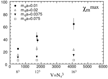
a) b)

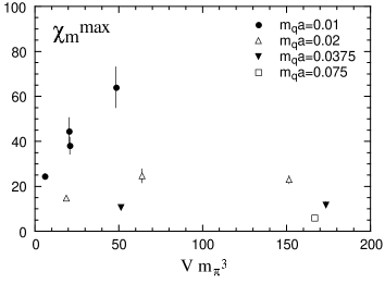
Fig. 10: (a) Peak height of the magnetic susceptibility for $N_{F}=2$ QCD with staggered quarks as a function of the spatial lattice volume $N_{s}^{3}$. (b) The same data as a function of the lattice volume rescaled by zero-temperature pion correlation length.

Possible causes of the discrepancy are (i) $m_{q}$ is not small enough to see the critical behavior in the chiral limit, and (ii) the spatial lattice volume is not large enough to obtain the observables in the thermodynamic limit. Two additional caveats are in order for $N_{F}=2$ staggered quarks: (iii) The symmetry in the chiral limit at $a>0$ is O(2) instead of O(4). Practically, however, the values of the O(2) exponents are almost indistinguishable from the O(4) values with the present numerical accuracy. (iv) The action is not local. Therefore, an assumption behind the universality argument can be violated so that some non-universal behavior may appear [13]. The correct continuum chiral limit with the O(4) symmetry will be obtained only when we first take the continuum limit $a\rightarrow 0$ and then take the chiral limit. In addition to these points, we also have to check technical details in the numerical simulation; the accuracy of the methods to simulate the system, such as the the finite step-size error and the dependence on the convergence criterion for fermion matrix inversion.

A systematic study of the quark mass dependence as well as the lattice volume dependence is in order. The JLQCD Collaboration performed a series of simulations on $8^{3}\times 4$, $12^{3}\times 4$, and $16^{3}\times 4$ lattices at $m_{q}a=0.01$, 0.02, 0.0375, and 0.075 [74]. The Bielefeld group also extended their study to larger spatial lattices [75]. The results obtained are consistent with each other. It turned out that determination of critical exponents on $8^{3}\times 4$ lattices suffers from a sizable finite lattice-size effect for $m_{q}a<0.0375$.

From the lattice-size dependence of the magnetic susceptibility $\chi_{m}$ for a fixed value of quark mass, shown in Fig. 10(a), we find that the transition is a crossover for $m_{q}a\geq 0.02$; the peak height $\chi_{m}^{\rm max}$ for $m_{q}a=0.02$ stabilizes on spatial lattices larger than $12^{3}$. For $m_{q}a=0.01$, on the other hand, $\chi_{m}^{\rm max}$ is increasing up to the largest spatial lattice of $16^{3}$. If this increase is maintained up to infinite volume, then the transition is first order at this quark mass. However, no clear indication of a first-order transition are found from the lattice volume dependence of Monte Carlo time histories and histograms at $m_{q}a=0.01$. Furthermore, when the lattice volume is rescaled by the zero-temperature pion correlation length, the lattice volume $16^{3}$ for $m_{q}a=0.01$ approximately corresponds to the volume $12^{3}$ for $m_{q}a=0.02$, where the increase of $\chi_{m}^{\rm max}$ terminates [see Fig. 10(b)]. Therefore, it is possible that the increase of $\chi_{m}^{\rm max}$ for $m_{q}a=0.01$ is a transient effect.

Assuming that the finite size effect is sufficiently small on the $16^{3}\times 4$ lattice, we fit the data at the four values of $m_{q}a$. We find $z_{g}=0.64(5)$, $z_{m}=1.03(9)$, and $z_{t}=0.82(12)$. (Removing the data for $m_{q}a=0.01$ gives slightly smaller but consistent values with larger errors.) The results for $z_{g}$ and $z_{m}$ deviate sizably from the O(2) or O(4) values. On the other hand, the identity $z_{g}+z_{m}-z_{t}=1$ expected for a second-order fixed point with two relevant operators is approximately satisfied. Thus, the exponents are consistent with a second-order transition at $m_{q}=0$.

In summary, we find that the determination of the nature of the two-flavor chiral transition with staggered quarks using the standard action to involve subtle problems. While the data so far do not contradict a second-order transition at $m_{q}=0$, the exponents take quite unexpected values, at least in the range $m_{q}a\geq 0.01$. Evidently further work, possibly on larger spatial sizes and smaller quark masses, is needed to clarify this important problem.

5.1.2 Results with Wilson quarks

Let us now study the issue using Wilson quarks. It turned out that Wilson quarks in the standard action lead to several unexpected phenomena on lattices with $N_{t}=4$ and 6: On these lattices, the transition becomes once very sharp when $m_{q}$ is increased from the chiral limit [76, 10], contrary to the expectation in the continuum limit that the chiral transition becomes weaker with larger $m_{q}$. Together with other strange behavior of physical quantities near the transition point, this phenomenon is identified as an effect of lattice artifacts [10].

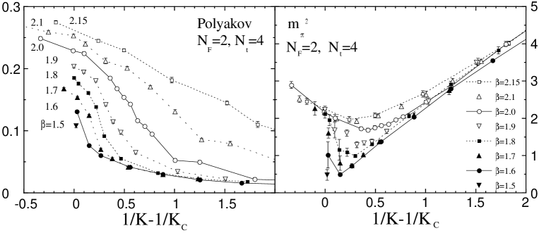
Fig. 11: The Polyakov loop and the pion screening mass obtained with Wilson quarks with a RG improved action [41]. In these figures, the conventional notation $\beta\equiv 6/g^{2}$ is used. Larger $\beta$ corresponds to a higher temperature. The horizontal axis $1/K-1/K_{C}$ is proportional to $m_{q}a$.

Therefore, the Tsukuba group applied an improved action [41]. Their action is the RG improved gauge action (3.8) with $c_{1}=-0.331$, coupled with the standard Wilson quark action. Although the quark part is not improved, the lattice artifacts observed with the standard action are shown to be well removed[41, 77]. They also find that the physical quantities are quite smooth around the transition point at $m_{q}>0$, as shown in Fig. 11. The straight line envelop of $m_{\pi}^{2}$ at finite temperature ($N_{t}=4$) shown in Fig. 11(b) agrees with $m_{\pi}^{2}$ obtained at low temperature ($N_{t}=8$), and corresponds to the PCAC relation $m_{\pi}^{2}\propto m_{q}$ expected in the low-temperature phase. The smoothness of the physical observables strongly suggests that the transition is a crossover at $m_{q}>0$.

Concerning the nature of the transition in the chiral limit, the transition becomes monotonically weaker with increasing $6/g^{2}$ (see Fig. 11). Because the transition point shifts to larger $6/g^{2}$ at larger $m_{q}$, increasing $6/g^{2}$ corresponds to increasing $m_{q}$ for the transition. In the chiral limit $m_{\pi}^{2}$ decreases monotonically to zero as the temperature is decreased from above, towards the chiral transition point. At the transition temperature for finite $m_{q}$, $m_{\pi}^{2}$ also shows a similar monotonic decrease with decreasing $m_{q}$. These results suggest that the chiral transition is continuous.

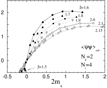
a) b)

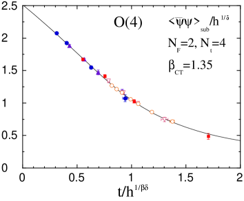
Fig. 12: (a) Chiral condensate as a function of $h=2m_{q}a$ for Wilson quarks with a RG improved action[41]. (b) Best fit for the scaling function with O(4) exponents with $\chi^{2}/df=0.61$, using the identification $h=2m_{q}a$ and $t=\beta-\beta_{ct}$, where $\beta\equiv 6/g^{2}$ and $\beta_{CT}$ is the value of $6/g^{2}$ at the chiral transition point. Do not confuse with the critical exponent $\beta$ appearing in the combination $t/h^{1/\beta\delta}$. The plot contains all data of (a) within the range $0<2m_{q}a<0.8$ and $6/g^{2}\leq 2.0$. Solid curve represents the scaling function obtained in an O(4) spin model.

For a more decisive test about the nature of the transition, a scaling study is required. From the universality argument, the magnetization $M$ in a spin model can be described by a single scaling function near a second order transition point:

$$M/h^{1/\delta}=f(t/h^{1/\beta\delta}),$$ (5.1)

where $h$ is the external magnetic field and $t=[T-T_{c}]/T_{c}$ the reduced temperature. When the QCD transition is of second order in the chiral limit, the chiral condensate should satisfy this scaling relation with O(4) exponents $1/\beta\delta=0.537(7)$ and $1/\delta=0.2061(9)$ [72] and also with the O(4) scaling function $f(x)$.

The magnetization $M$ is identified with the chiral condensate in QCD. For Wilson quarks, the naive definition of $\langle\bar{\psi}\psi\rangle$ for the chiral condensate is not adequate because the chiral symmetry is explicitly broken due to the Wilson term. A proper subtraction and a renormalization are required to obtain the correct continuum limit. A properly subtracted $\langle\bar{\psi}\psi\rangle$ can be defined via an axial Ward identity [7]:

$$\langle\bar{\psi}\psi\rangle_{\rm sub}=2m_{q}aZ\sum_{x}\langle\pi(x)\pi(0)\rangle$$ (5.2)

where $Z$ is the renormalization coefficient. For our purposes, it is enough to use the tree value, $Z=(2K)^{2}$. When the chiral symmetry is spontaneously broken, a singulariry in the pion propagator cancels the factor $m_{q}$ in the r.h.s. of (5.2), giving a finite value for $\langle\bar{\psi}\psi\rangle_{\rm sub}$ in the chiral limit.

The results of $M=\langle\bar{\psi}\psi\rangle_{\rm sub}$ around the deconfining transition/crossover for $N_{t}=4$ is shown in Fig. 12(a). Fig. 12(b) shows the result from a fit of $M$ to the scaling function obtained for an O(4) model [78], by adjusting the chiral transition point $\beta_{ct}$ and the scales for $t$ and $h$, with the exponents fixed to the O(4) values. The scaling ansatz works remarkably well with the O(4) exponents. A recent study shows that the situation holds also when data at $t\leq 0$ are included [77]. On the other hand, a change of the exponents quickly makes the fit worse: For example, fixing the exponents to the MF values, suggested by Kocić and Kogut as a possibility for two-flavor QCD[79], the data no longer falls on the MF scaling function.

The success of this scaling test with the O(4) exponents suggests strongly that the chiral transition is of second order in the continuum limit. It also indicates that the chiral violation due to the Wilson fermion action is sufficiently small with this improved action, for the values of $m_{q}$ and $6/g^{2}$ studied here.

5.2 Influence of the strange quark

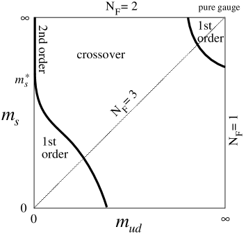
a) b)

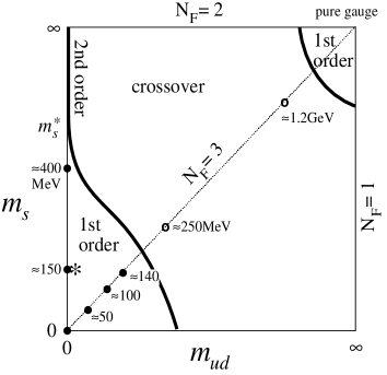
Fig. 13: (a) Map of expected nature of the QCD transition for $N_{F}=2+1$ QCD as a function of the u and d quark mass $m_{ud}$ and the s quark mass $m_{s}$. (b) The same figure with the results from Wilson quarks using the standard action [10]. First order signals are observed at the points marked by filled circles, while no clear two-state signals are found at the points represented by the open circles. The values of quark mass in physical units are computed using $a$ determined by $m_{\rho}(T\!=\!0)=770$ MeV. The real world corresponds to the point marked by the star.

In order to study the nature of the transition in the real world, we should study the influence of the s quark. Our expectation about the nature of the finite temperature transition as a function of quark masses is summarized in Fig. 13(a), neglecting the mass difference among u and d quarks ($N_{F}=2+1$). The limit $m_{s}=\infty$ corresponds to the case $N_{F}=2$ discussed in Sect. 5.1 where we found second order transition at $m_{ud}=0$. For $m_{ud}=m_{s}$ ($N_{F}=3$), the transition is of first order in the chiral limit. Therefore, on the axis $m_{ud}=0$, we have a tricritical point $m_{s}^{*}$ where the second order transition at large $m_{s}$ turns into first order [69]. For $m_{s}<m_{s}^{*}$, the second order edge of the first order transition region is suggested[80] to deviate from the vertical axis according to $m_{ud}\propto(m_{s}^{*}-m_{s})^{5/2}$. Our main goal of investigations with the s quark is to determine the position of the physical point in this map.

With staggered quarks, Brown et al. [81] found, for the degenerate $N_{F}=3$ case ($m_{ud}=m_{s}\equiv m_{q}$), a first order signal at $m_{q}a=0.025$, $\beta=5.132$. For $N_{F}=2+1$, they obtained a time history suggesting a crossover for $m_{ud}a=0.025$, $m_{s}a=0.1$ at $\beta=5.171$. Their study of hadron spectrum at this simulation point on a zero-temperature lattice leads to a $m_{K}/m_{\rho}$ smaller than the experimental value, suggesting that this $m_{s}$ is smaller than the physical value. At the same time, their large $m_{\pi}/m_{\rho}$ suggests that their $m_{ud}$ is larger than the physical value. This implies that the physical point is located in the crossover region unless the second order transition line, which has a sharp $m_{ud}$ dependence near $m_{s}^{*}$ (cf. Fig. 13(a)), crosses between the physical point and the simulation point. In order to obtain a more decisive conclusion, a study to systematically investigate a wider region of the parameter space in Fig. 13(a) is required.

The Tsukuba group studied the issue with Wilson quarks using the standard action [10]. They found first order signals for $m_{q}\mathop{\vtop{\halign{#\cr$\hfil\displaystyle{<}\hfil$\crcr\kern 0.5pt\nointerlineskip\cr$\sim$\crcr\kern 0.5pt\cr}}}\limits 140$ MeV, while no clear two state signals were observed for $m_{q}\mathop{\vtop{\halign{#\cr$\hfil\displaystyle{>}\hfil$\crcr\kern 0.5pt\nointerlineskip\cr$\sim$\crcr\kern 0.5pt\cr}}}\limits 250$ MeV, where the physical s quark mass, giving $m_{\phi}=1.02$ GeV, is about 150 MeV in their normalization of $m_{q}$. (The scale was fixed by $m_{\rho}$ at zero tmeperature.) For $N_{F}=2+1$, first order signals are observed for $m_{ud}\sim 0$ at both $m_{s}\sim 150$ and 400 MeV. A study of zero-temperature hadron spectroscopy for $N_{F}=2+1$ shows that $m_{\phi}\sim 1.03(5)$ GeV at the simulation point $m_{s}\sim 150$ MeV, verifying that this simulation point is very close to the physical point. The results are summarized in Fig. 13(b). The physical point is located in the first order region.

Although both staggered and Wilson simulations give a phase structure qualitatively consistent with Fig. 13(a), Wilson quarks tend to give larger values for critical quark masses (measured by $m_{\phi}/m_{\rho}$ etc.) than those with staggered quarks. This leads to the difference in the conclusions about the location of the physical point in Fig. 13(a). On the other hand, both of these studies discuss sizable deviation of several physical observables from the experimental values, meaning that the deviation from the continuum limit is large at $N_{t}=4$ where these simulations are done. We should certainly carry out a calculation at larger $N_{t}$ or with an improved action in order to draw a definite conclusion about the nature of the QCD transition in the real world.

6 Summary

With the present power of computers, we can perform reliable extrapolations to the continuum limit for several physical quantities in the quenched approximation of QCD. Precise values of the transition temperature, latent heat, interface tension, etc. obtained from detailed finite size scaling analyses are discussed in the literature. For full QCD simulations, however, several hundred times more computer time is required compared to quenched simulations. This corresponds to about 5–10 years difference in the development of computer speed. While a few projects to construct a computer with such a speed have been proposed, we are not simply waiting for new computers. Many theoretical developments, especially the progress in improving lattice actions, open us the possibility to begin realistic simulations of full QCD on present supercomputers. Applications of improved actions to full QCD at finite temperatures have just begun.[41, 77, 82, 83]

References

- [1] M. Creutz, “Quarks, Gluons and Lattices”, (Cambridge Univ. Press, 1983). H.J. Rothe, “Lattice Gauge Theories – An Introduction”, (World Sci., Lecture Notes in Physics Vol.43, 1992). I. Montvay and G. Münster, “Quantum Fields on a Lattice”, (Cambridge Univ. Press, 1994).
- [2] Proc. Lattice 97 [Nucl. Phys. B(Proc. Suppl.)63 (1998)]; Lattice 96 [ibid. 53 (1997)]; Lattice 95 [ibid. 47 (1996)]. For recent reviews on finite temperature lattice QCD, see A. Ukawa, Nucl. Phys. B(Proc. Suppl.)53 (1997), 106; E. Laermann, ibid. 63 (1998), 114.
- [3] K.G. Wilson, Phys. Rev. D10 (1974), 2445.
- [4] H.B. Nielsen and M. Ninomiya, Nucl. Phys. B185 (1981), 20; ibid. B193 (1981), 173.
- [5] K.G. Wilson, in New Phenomena in Subnuclear Physics, ed. A. Zichichi (Plenum, New York, 1977).
- [6] J. Kogut and L. Susskind, Phys. Rev. D11 (1975), 395.
- [7] M. Bochicchio, L. Maiani, G. Martinelli, G. Rossi and M. Testa, Nucl. Phys. B262 (1985), 331.
- [8] S. Itoh, Y. Iwasaki, Y. Oyanagi and T. Yoshié, Nucl. Phys. B274 (1986), 33.
- [9] CP-PACS Collaboration: S. Aoki et al., Nucl. Phys. B(Proc. Suppl.)63 (1998), 161; ibid. 60A (1998), 14.
- [10] Y. Iwasaki, K. Kanaya, S. Kaya, S. Sakai, and T. Yoshié, Phys. Rev. D54 (1996), 7010.
- [11] S. Aoki, Phys. Rev. D30 (1984), 2653; Phys. Rev. Lett. 57 (1986), 3136; Nucl. Phys. B314 (1989), 79.
- [12] S. Aoki, A. Ukawa, and T. Umemura, Phys. Rev. Lett. 76 (1996), 873. S. Aoki, Nucl. Phys. B(Proc. Suppl.)60A (1998), 206.
- [13] K. Kanaya, Nucl. Phys. B(Proc. Suppl.)47 (1996), 144.
- [14] N. Cabibbo and E. Marinari, Phys. Lett. B119 (1982), 387. M. Okawa, Phys. Rev. Lett. 49 (1982), 353.
- [15] A. Bartoloni et al., Nucl. Phys. B(Proc. Suppl.)63 (1998), 991.
- [16] D. Chen et al., Nucl. Phys. B(Proc. Suppl.)63 (1998), 997.
- [17] Y. Iwasaki, Nucl. Phys. B(Proc. Suppl.)60A (1998), 246. See also http://www.rccp.tsukuba.ac.jp/.
- [18] S. Duane, A.D. Kennedy, B.J. Pendleton and D. Roweth, Phys. Lett. B195 (1987), 216.
- [19] S. Gottlieb, W. Liu, D. Toussaint, R.L. Renken and R.L. Sugar, Phys. Rev. D35 (1987), 2531.
- [20] P. Hasenfratz, Nucl. Phys. B(Proc. Suppl.)63 (1998), 53. F. Niedermayer, ibid.53 (1997), 56.
- [21] G.P. Lepage, in the Proceedings of 1996 Schaladming Winter School on Perturbative and Nonperturbative Aspects of Quantum Field Theory (hep-lat/9607076).
- [22] K.G. Wilson, in “Recent Developments of Gauge Theories”, ed. G. ’tHooft et al. (Plenum, 1980).
- [23] K. Symanzik, Nucl. Phys. B226 (1983), 187; 205.
- [24] M. Lüscher and P. Weisz, Commun. Math. Phys. 97 (1985), 59; erratum, 98 (1985), 433.
- [25] P. Weisz, Nucl. Phys. B212 (1983), 1. P. Weisz and R. Wohlert, Nucl. Phys. B236 (1984), 397.
- [26] M. Alford, W. Dimm and G.P. Lepage, Phys. Lett. B361 (1995), 87. B. Beinlich, F. Karsch and E. Laermann, Nucl. Phys. B462 (1996), 415.
- [27] M. Lüscher and P. Weisz, Phys. Lett. 158B (1985), 250.
- [28] G.P. Lepage and P.B. Mackenzie, Phys. Rev. D48 (1993), 2250.
- [29] G. Parisi, in Proc. XX International Conference “High Energy Physics-1980”, ed. L. Durand and L. Pondrom, American Inst. of Physics (1981), 1531. F. Green and S. Samuel, Nucl. Phys. B194 (1982), 107. Yu.M. Makeenko and M.I. Polikarpov, Nucl. Phys. B205[FS5] (1982), 386. S. Samuel, O. Martin and K. Moriarty, Phys. Lett. B153 (1985), 87.
- [30] B. Sheikholeslami and R. Wohlert, Nucl. Phys. B259 (1985), 572.
- [31] P.B. Mackenzie, Nucl. Phys. B(Proc. Suppl.)30 (1993), 35.
- [32] M. Lüscher et al., Nucl. Phys. B491 (1997), 323.
- [33] P. Hasenfratz and F. Niedermayer, Nucl. Phys. B414 (1994), 785.
- [34] P. Hasenfratz, in these proceedings.
- [35] Ph. de Forcrand et al., Nucl. Phys. B(Proc. Suppl,)63 (1998), 928.
- [36] W. Bietenholz and U.-J. Wiese, Nucl. Phys. B464 (1996), 319. K. Orginos et al., Nucl. Phys. B(Proc. Suppl.)63 (1998), 904.
- [37] T. DeGrand et al., Nucl. Phys. B(Proc. Suppl.)53 (1997), 942.
- [38] Y. Iwasaki, Nucl. Phys. B258 (1985), 141. Univ. of Tsukuba report UTHEP-118 (1983), unpublished.
- [39] Y. Iwasaki, K. Kanaya, T. Kaneko, and T. Yoshié, Phys. Rev. D56 (1997), 151.
- [40] CP-PACS Collaboration: S. Aoki et al., Nucl. Phys. B(Proc. Suppl,)63 (1998), 221.
- [41] Y. Iwasaki, K. Kanaya, S. Kaya, and T. Yoshié, Phys. Rev. Lett. 78 (1997), 179.
- [42] A.M. Polyakov, Phys. Lett. B72 (1978), 477. L. Susskind, Phys. Rev. D20 (1979), 2610.
- [43] B. Svetisky and L.G. Yaffe, Nucl. Phys. B210[FS6] (1982), 423.
- [44] Y. Iwasaki, K. Kanaya, T. Yoshié, T. Hoshino, T. Shirakawa, Y. Oyanagi, S. Ichii, and T. Kawai, Phys. Rev. D46 (1992), 4657.
- [45] M. Fukugita, M. Okawa and A. Ukawa, Nucl. Phys. B337 (1990), 181
- [46] R.G. Edwards, U.M. Heller and T.R. Klassen, hep-lat/9711003.
- [47] G. Boyd et al., Phys. Rev. Lett. 75 (1995), 4169; Nucl. Phys. B469 (1996), 419.
- [48] T. DeGrand et al., Nucl. Phys. B454 (1995), 615.
- [49] D.W. Bliss, K. Hornbostel, and G.P. Lepage, hep-lat/9605041.
- [50] B. Beinlich, F. Karsch, E. Laermann and A. Peikert, hep-lat/9707023.
- [51] E. Eichten, K. Gottfried, T. Kinoshita, K.D. Lane and T.M. Yan Phys. Rev. D21 (1980), 203.
- [52] J. Engels, F. Karsch, H. Satz and I. Montvay, Nucl. Phys. B205 (1982), 545.
- [53] F. Karsch, Nucl. Phys. B205 (1982), 285.
- [54] R. Trinchero, Nucl. Phys. B227 (1983), 61. F. Karsch and I.O. Stamatescu, Phys. Lett. B227 (1989), 153.
- [55] QCDTARO Collaboration: K. Akemi et al., Phys. Rev. Lett. 71 (1993), 3063.
- [56] B. Beinlich, F. Karsch and A. Peikert, Phys. Lett. B390 (1997), 268.
- [57] G. Burgers, F. Karsch, A. Nakamura and I.O. Stamatesc, Nucl. Phys. B304 (1988), 587.
- [58] QCDTARO Collaboration: M. Fujisaki et al., Nucl. Phys. B(Proc. Suppl.)53 (1997), 426.
- [59] J. Engels, F. Karsch and T. Scheideler, Nucl. Phys. B(Proc. Suppl.)63 (1998), 427.
- [60] T.R. Klassen, hep-lat/9803010.
- [61] J. Engels, J. Fingberg, F. Karsch, D. Miller and M. Weber, Phys. Lett. B252 (1990), 625.
- [62] B. Beinlich, F. Karsch and E. Laermann, Nucl. Phys. B462 (1996), 415.
- [63] T. Blum, L. Kärkkäinen D. Toussaint and S. Gottlieb, Phys. Rev. D51 (1995), 5153.
- [64] S. Ejiri, Talk at YKIS97. S. Ejiri, Y. Iwasaki, K. Kanaya and T. Yoshié, “Non-perturbative determination of anisotropy coefficients in lattice gauge theories”, Tsukuba preprint UTCCP-P-36 (1998).
- [65] K. Binder, Z. Phys. B43 (1981), 119; Phys. Rev. A25 (1982), 1699.
- [66] Y. Iwasaki, K. Kanaya, L. Kärkkäinen, K. Rummukainen and T. Yoshié, Phys. Rev. D49 (1994), 3540.
- [67] B. Grossmann and M.L. Lauersen, Nucl. Phys. B408 (1993), 637.
- [68] A. Papa, hep-lat/9710091.
- [69] R. Pisarski and F. Wilczek, Phys. Rev. D29 (1984), 338. F. Wilczek, Int. J. Mod. Phys. A7 (1992), 3911. K. Rajagopal and F. Wilczek, Nucl. Phys. B399 (1993), 395.
- [70] Y. Iwasaki, K. Kanaya, S. Kaya, S. Sakai and T. Yoshié, “Quantum Chromodynamics with Many Flavors”, in these proceedings [Tsukuba preprint UTCCP-P-35 (1998)].
- [71] A. Ukawa, in the Proceedings of Uehling Summer School 1993 (World Sci., 1995).
- [72] K. Kanaya and S. Kaya, Phys. Rev. D51 (1995), 2404. P. Buetera and M. Comi, Phys. Rev. B52 (1995), 6185. H.G. Ballesteros, L.A. Fernández, V. Martín-Mayor and A. Muñoz Sudupe, Phys. Lett. B387 (1996), 125.
- [73] F. Karsch, Phys. Rev. D49 (1994), 3791. F. Karsch and E. Laermann, Phys. Rev. D50 (1994), 6954.
- [74] JLQCD Collaboration: S. Aoki et al., hep-lat/9710048 (to be published in Phys. Rev. D).
- [75] G. Boyd, F. Karsch, E. Laermann, and M. Oevers, in the Proceedings of “Problems of Quantum Field Theory”, May 1996, Crimea, Ukraine (hep-lat/9607046). E. Laermann, Nucl. Phys. B(Proc. Suppl.)60A (1997), 180.
- [76] C. Bernard et al., Phys. Rev. D49 (1994), 3574; ibid. D46 (1992), 4741. T. Blum et al., Phys. Rev. D50 (1994), 3377.
- [77] Y. Iwasaki et al., Nucl. Phys. B(Proc. Suppl.)42 (1995), 502. Y. Iwasaki et ai., Nucl. Phys. B(Proc. Suppl.)47 (1996), 515. S. Aoki et al., Nucl. Phys. B(Proc. Suppl.)63 (1998), 397.
- [78] D. Toussaint, Phys. Rev. D55 (1997), 362.
- [79] A. Kocić and J. Kogut, Phys. Rev. Lett. 74 (1995), 3112; Nucl. Phys. B455 (1995), 229.
- [80] K. Rajagopal, in Quark-Gluon Plasma 2, ed. R. Hwa (World Sci., 1995).
- [81] F.R. Brown et al., Phys. Rev. Lett. 65 (1990), 2491.
- [82] C. Bernard et al., Nucl. Phys. B(Proc. Suppl.)53 (1997), 446; Phys. Rev. D56 (1997), 5584.
- [83] J. Engels et al., Phys. Lett. B396 (1997), 210. A. Peikert et al., Nucl. Phys. B(Proc. Suppl.)63 (1998), 895.