HIP – 1998 – 19 / TH LTH – 422

Four-quark flux distribution and binding
in lattice SU(2)

P. Pennanen, A. M. Green^,

Helsinki Institute of Physics
$\,{}^{2}$Department of Physics
P.O. Box 9, FIN-00014 University of Helsinki, Finland

and C. Michael

Theoretical Physics Division, Dept. of Math. Sciences, University of Liverpool, Liverpool, UK.

The full spatial distribution of the color fields of two and four static quarks is measured in lattice SU(2) field theory at separations up to 1 fm at $\beta=2.4$. The four-quark case is equivalent to a $q\bar{q}q\bar{q}$ system in SU(2) and is relevant to meson-meson interactions. By subtracting two-body flux tubes from the four-quark distribution we isolate the flux contribution connected with the four-body binding energy. This contribution is further studied using a model for the binding energies. Lattice sum rules for two and four quarks are used to verify the results.

PACS numbers: 11.15.Ha, 12.38.Gc, 13.75.-n, 24.85,+p

1 Introduction

Monte Carlo simulations of lattice gauge theory are among the most powerful tools for investigating non-perturbative phenomena of QCD such as confinement. The potential $V(R)$ between two static quarks at separation $R$ in quenched QCD is a simple manifestation of confinement and has been studied intensively. At large $R$ the potential rises linearly as predicted by the hadronic string model. One can also measure the spatial distribution of the color fields around such static quarks in order to get a detailed picture of the confining flux tube. In Refs. [1, 2], which contain references to earlier work, this was done for the ground state and two excited states of the two-quark potential. Transverse and longitudinal profiles of chromoelectric and -magnetic fields were compared with vibrating string and dual QCD models for the flux tube, with the latter model reproducing quite well the shape of the energy profile measured on a lattice. Instead of SU(3), the gauge group used was SU(2), which is more manageable with present-day computer resources and is expected to have very similar features of confinement. This is reflected in the fact that the flux tube models considered do not distinguish between SU(2) and SU(3) and in the small $N_{c}$ dependence observed in the spectrum of pure gauge theories [3].

A more complicated situation is encountered with multi-quark systems, which are abundant in nature and whose understanding from first principles, i.e. from QCD, is at present very limited. This is mainly due to the failure of perturbation theory in this intermediate energy domain and the heavy computer requirements for Monte Carlo simulations. The simplest multi-quark system, this meaning more than a single meson or baryon, consists of four quarks and occurs e.g. in meson-meson scattering and bound states. Understanding the four-quark interaction would be the first step in deriving nuclear physics from QCD. Previously, static four quark systems have been extensively simulated in SU(2) lattice gauge theory and a phenomenological potential model containing a many-body interaction term $f$ has been developed to explain the observed binding energies [4, 5, references therein]. Here binding energies, which have values up to $\approx 100$ MeV, mean $E_{4}-[V_{2}(a)+V_{2}(b)]$, where $E_{4}$ is the total energy of four quarks and $V_{2}(a)+V_{2}(b)$ the energy of the lowest lying pairings ’$a$’ and ’$b$’ of the quarks. This so-called $f$-model with four independent parameters, and including the effect of excited gluonic states, has been found in Refs. [6, 7] to reproduce 100 measured energies of the six types of four-body geometries we have simulated.

In order to gain more insight into the binding of multi-quark systems we now look at the microscopic properties of the color fields around four static quarks. We are not aware of any serious theoretical model for the fields in this case. For this first study we treat a geometry where the quarks sit at the corners of a square. This geometry was chosen mainly because a simple version of the $f$-model using only two-body ground state potentials reproduces the observed binding energies.

This paper is organised as follows: The method we use to measure the fields is first presented in Sect. 2 along with the details of our simulation and data analysis techniques. The resulting potentials and binding energies are discussed in Sect. 3. These are input for the two- and four-body lattice sum rules presented in Sect. 4 which relate the energies to sums over flux distributions and help us to see when the measurement of the latter is accurate. Using the results from the sum rule check as a guide, flux distributions before and after subtracting two-body flux tubes from the four quark distribution are shown in Sect. 5. In Sect. 6 we analyse the fields using the simple $f$-model, and Sect. 7 contains our conclusions.

2 Measurement method

2.1 Color fields

The method used to study the color fields on a lattice is to measure the correlation of a plaquette $\Box\equiv{1\over N}{\rm Tr}U_{\Box}$ with the Wilson loop $W(R,T)$ that represents the static quark and antiquark at separation $R$. When the plaquette is located at $t=T/2$ in the $\mu,\ \nu$ plane, the following expression isolates, in the limit $T\to\infty$, the contribution of the color field at position ${\bf r}$:

$$f_{R}^{\mu\nu}({\bf r})=\left[{\langle W(R,T)\Box^{\mu\nu}_{\bf r}\rangle}-\langle W(R,T)\rangle\langle\Box^{\mu\nu}\rangle\over{\langle W(R,T)\rangle}\right].$$ (1)

Here $\langle\Box\rangle$ is taken in the gauge vacuum. Like all the other expectation values, it is averaged over all lattice sites.

In the naive continuum limit these contributions are related to the mean squared fluctuation of the Minkowski color fields by

$$f_{R}^{ij}({\bf r})\rightarrow-\frac{a^{4}}{\beta}B^{2}_{k}({\bf r})\quad{\rm with}\ i,\ j,\ k\ {\rm cyclic\ \ \ and}\quad f_{R}^{i4}({\bf r})\rightarrow\frac{a^{4}}{\beta}E^{2}_{i}({\bf r}).$$ (2)

The squares of the longitudinal and transverse electric and magnetic fields are identified as as

$${\cal E}_{x}=f^{41},\;{\cal E}_{y}=f^{42},\;{\cal E}_{z}=f^{43},\;{\cal B}_{x}=f^{23},\;{\cal B}_{y}=f^{31},\;{\cal B}_{z}=f^{12},$$ (3)

where the indices $1,2,3,4$ correspond to the directions $x,y,z,t$.

These can then be combined naively to give the action density

$$S({\bf r})=\sum_{i}({\cal E}_{i}+{\cal B}_{i})$$ (4)

and the energy density

$$E({\bf r})=\sum_{i}({\cal E}_{i}-{\cal B}_{i})$$ (5)

of the gluon field.

In the special case of two quarks lying on the same lattice axis, chosen here as the $x$-axis, we can identify the squares of the longitudinal and transverse electric and magnetic fields as

$${\cal E}_{L}={\cal E}_{x},\;{\cal E}_{T}={\cal E}_{y,z}\;{\rm and}\;{\cal B}_{L}={\cal B}_{x},\;{\cal B}_{T}={\cal B}_{y,z}.$$ (6)

Because the lattice breaks rotational symmetry, the fields were measured everywhere in space instead of only on the transverse lattice axis as in previous simulations. In Sect. 6 the flux tubes for quarks at the opposite corners of a square are also needed. However, assuming rotational invariance and interpolating on-axis results to off-axis (diagonal) points would introduce some error into the subtraction of two-body distributions from the four-body ones and render the results less reliable. The measured lack of rotational invariance of a $R=2$ on-axis flux tube is illustrated in Fig. 1 a) for the action density at $T=3$ in the transverse plane through a color source (i.e. at the quark). The contour lines are drawn using interpolation in units of GeV/fm³. These values in physical units are obtained by scaling the dimensionless lattice values by $\beta/a^{4}$, which equals $\approx 2418$ GeV/fm³ in this case. In Fig. 1 a) the rotational invariance is seen to be good except at the shortest distances; e.g. the value of the action density at point $(1,1)$ is achieved on-axis at a distance some 15% longer, while the $(2,2)$ value is achieved at about the same distance.

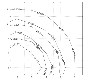
Figure 1: Lack of rotational invariance as illustrated by the action density at $T=3$ in the transverse plane at the quark for a) a two-body on-axis flux tube with separation $R=2$ and b) a two-body diagonal tube with separation $R=2,2$.

A similar plot for the corresponding off-axis tube is shown in Fig. 1 b). Because of the diagonal orientation of the tube on the lattice, the lattice spacings in the figure are different in the horizontal and vertical directions; on the horizontal axis they are $\sqrt{2}$ times the normal lattice spacing on the vertical axis. This is because the direction perpendicular to the line connecting the diagonal quarks, and in the same plane as the quarks, is also diagonal the lattice. For this off-axis situation the lack of rotational invariance seems to persist to longer distances. For example, the value marked by the outermost contour line at a distance of $\sqrt{10}$ is obtained at a distance about 10% longer on the horizontal axis. This suggests that significant error can be introduced if an on-axis flux tube is interpolated to an off-axis situation, or an off-axis tube is measured only on the transverse lattice axis.

The parts of the fields symmetrical with respect to the quarks were averaged in the measurement. For the two-body on-axis case this meant 16-fold averaging; each transverse plane has eight-fold symmetry, and the transverse planes with equal distance from the center of the quarks are the same. In the case of an off-axis flux tube the symmetry is only eight-fold due to the different lattice spacings in the two directions. For four quarks at the corners of the square we again have 16-fold symmetry; the quark plane is divided into eight symmetrical parts, and the parts above and below this plane are the same.

The quark distances we measured were $R=2,4,6,8$. For all these values, the energy and flux distribution measurement was performed for
a) two quarks on a lattice axis separated by $R$ lattice units,
b) two quarks on an axis diagonal with respect to the lattice axis and separated by $\sqrt{2}R$ units and
c) four quarks at the corners of a square with side length $R$.
Fig. 2 shows the measured areas in these three cases. In the on-axis case the microscopically measured volume consisted of 7 transverse planes at zero to six lattice units away from the center point in between the quarks, each covering a $6\times 6$ area with the region above the diagonal line removed because of symmetry. For the diagonal case 12 (diagonal) transverse planes of size $4\times 6$, starting $6\sqrt{2}$ lattice units away from the center point were measured. In the four-quark case we had 7 planes parallel to the quark plane and zero to six units outside it, each covering a $9\times 9$ area with the region above the diagonal line again removed. For the smaller $R=2$ system only 5, 8 planes were included in the on-axis and diagonal cases respectively, while in the four-quark case each plane covered only a $7\times 7$ area.

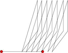
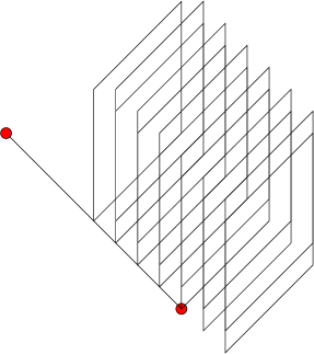
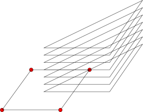
Figure 2: Area used for flux distribution measurement in the a) on-axis, b) diagonal and c) four-quark cases. The quarks are placed at $R=8$.

In addition to extracting the detailed structure of the color fields in space, there is also interest, when discussing sum rules, in the integrated values of these fields. Therefore we added the contributions from all measured points to get these integrated values. This is referred to as “sum 1” in Sect. 4 of this paper. In the simulations we also calculated the correlation of the total sum of all plaquettes on the lattice and the Wilson loop, and this will be referred to as “sum 2” below. The latter sum, therefore, includes a much larger volume than sum 1 and so should be a more realistic estimate. However, its error is expected to be larger due to the larger number of points.

2.2 Lattice operators for quarks

To explore the color fields around static quarks we need to find efficient lattice operators to represent the creation and destruction of the quarks. Here “efficient” means that the operators have a large overlap with the state we want to study and small overlap with other states. We use the same approach as previously when such operators were constructed for the measurement of the energies of two- and four-body systems. Each spatial link on the lattice is fuzzed, i.e. replaced by a normalised sum of $c$ times the link itself plus the surrounding four spatial U-bends or “staples”. Previous experience shows that $c=4$ is suitable. This is performed iteratively a number of times (the fuzzing level) until the operator is efficient.

By performing the measurements on lattices with different levels of fuzzing we obtain a variational basis, which is important for the minimization of the excited state contamination to the ground state signal. As we do not need information on the first excited two-body state with the same symmetry as the ground state, we are not worried by the fact that this second state, which we obtain after diagonalising our basis, also contains sizeable effects from the higher excited states as it effectively shields the ground state from too much contamination. The first excited state ($A_{1g}^{\prime}$) with ground-state symmetry has been studied in Ref. [2] using a three-state basis.

In the two quark case we initially used fuzzing levels 2 and 13. This choice gives good estimates of all 2-quark energies, even for the $R=8$ off-axis quark pair of length $8\sqrt{2}$ – the largest quark separation for the geometries considered. However, for the 2-quark flux tube profiles a problem emerged for this longest diagonal tube. At the midpoint of the tube the profile exhibited a valley – a feature not seen in any of the shorter tubes. This apparently arises, since the operator representing the diagonal flux tube is constructed from two L-shaped paths and our highest fuzzing level 13 was apparently not able to adequately reach the center of the L-shaped paths with side length 8 at $T=3,4$ – for higher $T$’s no useful signal was obtained. Changing the higher fuzzing level from 13 to 40 in a test run somewhat alleviated the problem, but our estimate of excited state contamination calculated from the energies and presented below in Table 3 of Sect. 3 did not show a significant decrease with this change in the fuzzing level. This further highlights how the inadequacy of the variational basis was only visible in the flux distribution and not in the energies, i.e. variational principles can give good energies but poor wavefunctions.

Unfortunately this change of fuzzing levels was still not enough to get a realistic signal in all cases for $R=8$. This would have required using a variational basis where the paths to be fuzzed were not simply L-shaped but closer to the diagonal in shape. Therefore, in the following, we did not use the $R=8$. For $R=6$ the transverse shape of the action in the diagonal flux tube was qualitatively correct, but even so it was still some $30\%$ lower in the middle than expected from the on-axis result.

For the case of four quarks the variational basis is obtained from the different ways to pair the four quarks, shown in Fig. 3, all at the same fuzzing level. For $R=2,4,8$ ($6$) we used fuzzing level 13 (40). With three basis states in hand we might have obtained better information on the first excited state, whose wavefunction is essentially $(|A\rangle-|B\rangle)/\sqrt{2}$. However, for the ground state [basically $(|A\rangle+|B\rangle)/\sqrt{2}$] the two and three basis state results are identical as was found earlier for the energies [4]. Thus we used only two basis states $A,B$ in most of the runs.

	A	B	C

Figure 3: Three ways to pair four quarks in the case of two colors.

2.3 Variance reduction

As there are many observables, each involving delicate cancellations, getting a good signal requires a large amount of computer time. One way to achieve this more easily is the so-called multihit or link integration method [8], where the statistical fluctuation of links in the Wilson loops is reduced by replacing the links by their thermal average. For calculating the expectation value of the link $U_{n\vec{\mu}}$ we only need to consider the part of the action involving this link – for the usual Wilson action, which uses just the plaquette operator, this is the sum $W$ of the six U-bends (staples) surrounding the link. In the case of SU(2) it can be shown that

$$<U_{n\vec{\mu}}>=\frac{\int dU_{n\vec{\mu}}U_{n\vec{\mu}}e^{-\frac{1}{N}\beta{\rm Tr}(UW^{\dagger})}}{\int dU_{n\vec{\mu}}e^{-\frac{1}{N}\beta{\rm Tr}(UW^{\dagger})}}=\frac{1}{d}\frac{I_{2}(\beta d)}{I_{1}(\beta d)}W,\;\;\;d={\rm det}W,$$ (7)

where the $I_{n}$’s are modified Bessel functions [9]. Their values were integrated numerically and stored as an array of 5000 points, the values given by analytical integration differing in the 7th or 8th decimal place. Using denser arrays did not change the Wilson loop correlations to an accuracy of 6 decimal places. The expectation value of a link is a real number times an SU(2) matrix, and the real numbers have to be stored for calculating correlations. The multi-hit algorithm cannot be used concurrently for links which are sides of the same plaquette, as the surrounding staples are kept fixed.

In our case we used multihit only on the time-like links of the Wilson loops. It is also possible to multihit all links of the Wilson loop and also the plaquette, but then the algorithm needs to be modified with several exceptions to avoid the problem just mentioned; this is discussed in Ref. [10]. The variance reduction we observe is presented in Table 1 for fuzzing levels 0,16,40 – the results for levels 2,13 being similar. These test runs used a $16^{3}\times 32$ lattice. As expected, the observed error reduction increases with time separation, as more links are then multi-hit. The reduction is also larger when the observables involve delicate cancellations; the error on the flux distributions calculated using Eq. 1 is reduced more than the error on the Wilson loop. In fact, as seen in the first four rows of the table, for the latter the effect is negligible. A rough estimate given in Ref. [11] of the error reduction for an unfuzzed Wilson loop by a factor of $(0.8)^{n}$ with $n$ links multihit, giving 0.26 for $T=3$ and 0.17 for $T=4$, is seen to be larger than what we observe for potentials obtained by diagonalizing a basis consisting of fuzzed loops.

An interesting question is the effect on the errors of multi-hit versus the choice of the variational basis. This is compared in Table 2 for the flux observables presented in the last eight rows of Table 1. In Table 2 “average error” refers to the average of the errors on the flux distribution measurements in Table 1 (and the corresponding one for fuzz levels 2,13). The error reduction is calculated both as the ratio of the average error with or without multihit and as the average of the error reductions of the field measurements in Table 1. The bottom row shows for the two choices of fuzzing levels the ratios of the time consumptions and the average errors. The choice of the variational basis can be seen to reduce errors by a magnitude comparable to the multi-hit algorithm. Switching off the use of multi-hit for the fuzzing level 2,13 case leads to a reduction in computing time by a factor of 0.90. This means that not using multi-hit on the time-links of the Wilson loop takes, in this case, 50% more computing time to achieve the same accuracy. This is a significant saving, but not as large as we first hoped would be achieved.

	error
observable	without	with	reduction
Potential, $R=4$, $T=3$	0.19 %	0.19 %	0.99
Potential, $R=4$, $T=4$	0.22 %	0.22 %	1.00
Potential, $R=8$, $T=3$	0.34 %	0.33 %	0.98
Potential, $R=8$, $T=4$	0.56 %	0.52 %	0.93
Action, $R=4$, $T=3$	1.19 %	0.73 %	0.61
Energy, $R=4$, $T=3$	2.21 %	1.59 %	0.72
Action, $R=4$, $T=4$	1.63 %	1.02 %	0.63
Energy, $R=4$, $T=4$	1.94 %	1.30 %	0.67
Action, $R=8$, $T=3$	3.70 %	2.91 %	0.79
Energy, $R=8$, $T=3$	6.68 %	6.30 %	0.94
Action, $R=8$, $T=4$	6.38 %	4.89 %	0.77
Energy, $R=8$, $T=4$	8.02 %	6.72 %	0.84

Table 1: Error reduction with multihit for potentials and flux in the center of $R=4,8$ flux tubes with fuzz levels 0,16,40. Errors are scaled to 1000 measurements.

		average error
Basis	time	without	with	ratio	average of reductions
0 16 40	7803 s	3.97 %	3.18 %	0.80	0.75
2 13	4108 s	4.81 %	3.70 %	0.77	0.78
ratio	0.52	0.83	0.86

Table 2: Error reduction with multihit and error reduction for a different variational basis, all for the same number of measurements (see text).

When the fields at or next to the color sources are measured, the plaquette touches the Wilson loop. In this case we cannot have any common link multihit in the Wilson loop and not multihit in the plaquette, as then we would use two different values of the same link in the same observable. Therefore, for correct measurements of the quark self-energies, which involve these links, we need to store versions of the Wilson loops with the appropriate links not multihitted. Neglecting this complication has resulted in erroneous measurements at the color sources in previous works [12].

Previously, a group in Wuppertal has measured four-quark flux distributions in SU(2) (unpublished and private communication). They employed a higher $\beta$ value and used larger lattices. However, their work is less suited for understanding the binding as the multihit algorithm was not switched off when a plaquette touched the Wilson loop, leading to unreliable self-energy measurement as discussed above. In addition, their diagonal flux tube was not measured directly, but instead the results for the on-axis tube, measured only on the transverse axis and not in full space, were interpolated to an off-axis situation. Also, no variational basis was employed for determining the two-body ground state. In view of the problem with our variational basis for the diagonal paths mentioned above it is not clear if the interpolation from the on-axis case does indeed produce worse results for the diagonal tube for large $R$’s.

2.4 Details of the simulation and analysis

The correlations in Eq. 1 were measured on a $20^{3}\times 32$ lattice with maximal time separation of the Wilson loops set to six lattice spacings. We averaged over all positions and orientations of the loops to improve statistics. The measurements were separated by one heatbath and three over-relaxation sweeps. Each measurement generated 4 MB of data and consumed 90 minutes of CPU time on a Cray C94 vector supercomputer. Sixteen or eight measurements were averaged into one block for $R=2,4$ and $R=6,8$ respectively, and 28 of these blocks were used for the final analysis. There the errors were estimated by using 100 bootstrap samples.

3 Energies and excited state contamination

The observed two-body potentials and four-quark binding energies, presented below in Tables 4–6, agree with previous results [4, references therein].

Since we use plaquettes in the middle of fuzzed Wilson loops in the time direction, we would like to know the excited state contamination at $t=T/2$. To estimate this contamination we use the method introduced for two-body potentials in Ref. [13]. From the Wilson loop ratios at each $R$-value, we define the effective two-body potential $V(T)=-\ln[W(T)/W(T-1)]$, since its rate of approach to a plateau as $T\to\infty$ enables us to estimate the excited state contamination to the ground state. A measure of this contamination is defined as

$$h(t)={c_{1}\over c_{0}}e^{-(V_{1}-V_{0})t}\ ,$$ (8)

which should be $\ll 1$. Here $V_{0}$ is the ground state potential and $V_{1}$ the potential of the first excited state with the same symmetry, and the $c_{i}$’s come from expanding a link operator that represents the creation or annihilation of two quarks at separation $R$ as $|R\rangle=c_{0}|V_{0}\rangle+c_{1}|V_{1}\rangle+\dots$ in terms of transfer matrix eigenstates. In practice $h$ is calculated from

$$|h(t=T/2)|\approx\frac{\lambda}{\lambda-1}\sqrt{V(T-1)-V(T)}=\lambda\frac{V(T-1)-V(T\rightarrow\infty)}{\sqrt{V(T-1)-V(T)}}.$$ (9)

Here the $T\rightarrow\infty$ extrapolated potential is defined as

$$V(T\rightarrow\infty)\equiv V(T)-\lambda\frac{V(T-1)-V(T)}{1-\lambda},\ \lambda\equiv e^{-(V_{1}-V_{0})}.$$

Table 3 shows the excited state contamination for the ground state of the two-body potential. The contamination at $t=1$ is calculated both from $T=1,2$ and $T=3,4$, the difference in the values reflecting the error in our estimates.

The contamination in the flux at $T$ is measured by $h(T/2)$, which should be small (e.g. $<0.1$). This suggests problems in the $R=8$ case, as already discussed in Sect. 2.2. In this case for $T=4$ the contamination is smaller, but the signal is then too noisy. In general, the consistency of results at larger $T$’s suggests that the effect from excited states is negligible.

	$R$	$t=1$ (a)	$t=1$ (b)	$t=1.5$	$t=2$
Fuzz levels 2 and 13
two-body	2	0.024	0.039	0.013	0.007
	4	0.065	0.071	0.030	0.019
	8	0.138	0.093	0.048	0.034
	2,2	0.035	0.048	0.015	0.009
	4,4	0.074	0.058	0.024	0.015
	8,8	0.273	0.078	0.051	0.039
Fuzz levels 2 and 40
two-body	4	0.079	0.105	0.038	0.028
	6	0.085	0.138	0.049	0.030
	8	0.159	0.155	0.061	0.051
	4,4	0.094	0.098	0.037	0.025
	6,6	0.113	0.107	0.043	0.025
	8,8	0.227	0.104	0.046	0.040

Table 3: Excited state contamination as measured by $h$. $t=1$ (a) refers to values calculated using $T=1,2$ energies, $t=1$ (b) to values using $T=3,4$ energies.

4 Sum rules for four static quarks

When a plaquette is used to probe the color flux with the Wilson gauge action, exact identities can be derived for the integrals over all space of the flux distributions. These sum rules [14, 15] relate spatial sums of the color fields measured using Eq. 1 to the energies of the system via generalised $\beta$-functions, which show how the bare couplings of the theory vary with the generalised lattice spacings $a_{\mu}$ in four directions. One can think of the sum rules as providing the appropriate anomalous dimension for the color flux sums. This normalises the color flux and provides a guide for comparing color flux distributions measured at different $a$-values. The full set of sum rules [15] allow these generalised $\beta$-functions to be determined at just one $\beta$-value [2, 13, and references therein].

A starting point for the sum rules is the identity

$$-{dE\over d\beta}=<1\,|\sum\Box|\,1>-<0\,|\sum\Box|\,0>=\sum\Box_{1-0},$$ (10)

derived in Ref. [14], which holds for ground-state energies $E$ obtained from the correlation of Wilson loops in the limit of large time separation. In Eq. 10 the symbol $\Box$ is the plaquette action ${1\over N}{\rm Tr}U_{\Box}$ which is summed over all plaquettes in a time slice, and the subscript $1-0$ refers to the difference of this sum in a state containing the observable system (1) and in the vacuum (0). For potentials between static sources the energy $E$ includes an unphysical lattice self-energy contribution which diverges in the continuum limit.

These relations can be trivially extended to the case of four static quarks. For a general configuration of four quarks the dimensionless energy $E(X,Y,Z,\beta)$ is a function of the coupling $\beta$ multiplying the plaquette action and distances in lattice units $X,Y,Z$ with physical lengths being $x=Xa$, $y=Ya$, $z=Za$, where $a$ is the lattice spacing. To remove the $\beta$-derivative from Eq. 10 we need to use the independence of a physical energy $E_{p}/a$ of $a$ as $a\rightarrow 0$ when $x,y,z$ are kept constant. That is, combining

$$0 = \left.{dE_{p}[x,y,z,\beta(a)]/a\over da}\right|_{x,y,z}$$

$$= -{E_{p}\over a^{2}}-\left.{X\over a^{2}}{\partial E_{p}\over\partial X}\right|_{Y,Z}-\left.{Y\over a^{2}}{\partial E_{p}\over\partial Y}\right|_{X,Z}-\left.{Z\over a^{2}}{\partial E_{p}\over\partial Z}\right|_{X,Y}+{1\over a}{d\beta\over da}\,\left.{\partial E\over\partial\beta}\right|_{X,Y,Z}$$

with Eq. 10 we get

$$E(x,y,z)+{\partial E\over\partial\ln X}+{\partial E\over\partial\ln Y}+{\partial E\over\partial\ln Z}+E_{0}=-{d\beta\over d\ln a}\,\sum\Box_{1-0},$$ (12)

where, unlike the physical energy, $E_{0}$ is a contribution from the unphysical self-energy that depends on $\beta$ and is not independent of $a$ in the continuum limit.

In the general case there are lattice spacings $a_{i}$ for all four directions $i=1,\ldots,4$, and couplings $\beta_{ij},\;i>j$ for all 6 orientations of a plaquette. As in Sect. 2, plaquettes with orientation 41,42,43,23,31,12 are labelled with ${\cal E}_{x},{\cal E}_{y},{\cal E}_{z},{\cal B}_{x},{\cal B}_{y},{\cal B}_{z}$ respectively. When $a_{i}=a$ for all $i$, derivatives of the couplings with respect to the lattice spacings fall into two classes

$${\partial\beta_{ij}\over\partial\ln a_{k}}=S\ \hbox{if}\ k=i\ \hbox{or}\ j\ \ \hbox{and}\ \ {\partial\beta_{ij}\over\partial\ln a_{k}}=U\ \hbox{if}\ k\neq i\ \hbox{or}\ j.$$ (13)

Using these equations and the invariance of $\frac{1}{a_{0}}E_{p}[X,Y,Z,\beta_{ij}(a_{k})]$ with respect to $a_{0}$, $a_{x}$, $a_{y}$, $a_{z}$ – in analogy to Eq.  4 – we get

$$E+E_{0}^{0} = -\sum S({\cal E}_{x}+{\cal E}_{y}+{\cal E}_{z})+U({\cal B}_{z}+{\cal B}_{y}+{\cal B}_{x})$$ (14)

$$X{\partial E\over\partial X}+E_{0}^{X} = -\sum S{\cal E}_{x}+U{\cal E}_{y}+U{\cal E}_{z}+S{\cal B}_{z}+S{\cal B}_{y}+U{\cal B}_{x}$$ (15)

$$Y{\partial E\over\partial Y}+E_{0}^{Y} = -\sum U{\cal E}_{x}+S{\cal E}_{y}+U{\cal E}_{z}+S{\cal B}_{z}+U{\cal B}_{y}+S{\cal B}_{x}$$ (16)

$$Z{\partial E\over\partial Z}+E_{0}^{Z} = -\sum U{\cal E}_{x}+U{\cal E}_{y}+S{\cal E}_{z}+U{\cal B}_{z}+S{\cal B}_{y}+S{\cal B}_{x}.$$ (17)

As for the $E_{0}$ in Eq. 12, the $E_{0}^{i}$’s on the LHS of these equations are self-energy contributions independent of $X,Y,Z$. Due to the isotropic nature of the self-energies we expect $E_{0}^{X}=E_{0}^{Y}=E_{0}^{Y}$. The negative sign on the RHS arises from our sign convention for the plaquette. In the case of a planar geometry, like the square we are now measuring, there is no extent in the direction perpendicular to the plane. If we choose this direction to be $z$, then Eq. 17 only has a self-energy term on the LHS.

In Ref. [2] the generalized $\beta$-functions $b\equiv\partial\beta/\partial\ln a=2(S+U)$ and $f\equiv(U-S)/(2\beta)$ were determined from two-body potentials and flux distributions using sum rules. From the best estimates of $b=0.312(15)$ and $f=0.65(1)$ at $\beta=2.4$ we get $S=-1.638(25),\;U=1.482(25)$ for Eqs. 14–17. Therefore, using the results for self-energies and -actions from Ref. [2], we get $E_{0}^{0}=0.14(5)$ – a number of interest when discussing Tables 4,5. With these values in hand we can use the above sum rules as a check on our flux distribution measurement.

Tables 4,5 shows the observed energies and corresponding energy sums for two and four quarks, respectively. Here “sum 1” means a sum over our microscopic measurements of the flux distribution, whereas “sum 2” denotes the correlation between the sum of all the plaquettes on the lattice and the Wilson loop(s). When our estimate of $E_{0}^{0}$ ($2E_{0}^{0}$) is added to the two (four) -body energies, the energy sums can be seen to agree with the observed energies especially for $T=2$.

The term $E_{0}^{0}$ can be removed by considering differences of flux-distributions, since then the self-energies cancel. Here we consider two such differences to be used later for a model of the binding energies; a) diagonal flux tubes subtracted from one-half times the flux tubes along the sides – $[F(AB)-F(C)]$ in Eq. 24 below – and b) one-half times the flux tubes along the sides of the square subtracted from the four-body distribution – $FB(4)$ in Eq. 24. These are shown in Table 6. In the first rows the differences of diagonal and on-axis potentials $V(R)-V(R,R)$ are compared to the difference of corresponding energy sums 1 and 2 in Table 4. The last rows contain four-body binding energies with a similar comparison. The agreement of these sums and the corresponding energy differences suggests correctness of our flux distribution measurement and subtractions, and proper cancellation of the self-energy distributions. One might expect the agreement of sum 2 with the energies to be slightly better than that of sum 1, since the area of our microscopic measurement always leaves a small tail-end of the signal unmeasured. In practice larger errors on sum 2 overcome this benefit in many cases. All the errors in these tables are from a bootstrap analysis.

We use Table 6 as a guide in the following for choosing the best $T$ value at which to look at the flux distribution measurement. The $R=4,6,8$ four-body binding energies and corresponding flux sums agree much better at $T=2$ than at higher $T$’s, where the large errors make the signal often consistent with zero. Therefore we use $T=2$ for these $R$’s and $T=3$ for $R=2$.

	$R$	observable	$T=2$	$T=3$	$T=4$
two-body	2	potential	0.56347(41)	0.56246(47)	0.56217(51)
		sum 1	0.4307(36)	0.4668(44)	0.4504(54)
		sum 2	0.443(17)	0.490(24)	0.487(32)
	2,2	potential	0.67123(79)	0.66954(97)	0.6689(11)
		sum 1	0.5216(77)	0.574(10)	0.548(12)
		sum 2	0.540(28)	0.610(42)	0.601(57)
	4	potential	0.78314(55)	0.77806(71)	0.77594(85)
		sum 1	0.6057(92)	0.685(14)	0.657(17)
		sum 2	0.640(26)	0.740(41)	0.692(49)
	4,4	potential	0.9267(10)	0.9178(13)	0.9144(15)
		sum 1	0.687(25)	0.822(37)	0.771(50)
		sum 2	0.759(57)	0.913(76)	0.914(15)
	6	potential	0.9454(16)	0.9368(18)	0.9336(20)
		sum 1	0.730(30)	0.832(52)	0.828(77)
		sum 2	0.780(81)	0.90(12)	0.86(17)
	6,6	potential	1.1567(32)	1.1346(32)	1.1268(39)
		sum 1	0.961(74)	1.08(12)	1.07(16)
		sum 2	1.01(17)	1.06(26)	0.86(36)
	8	potential	1.1293(15)	1.1077(22)	1.0968(34)
		sum 1	0.874(50)	1.008(65)	0.92(13)
		sum 2	0.88(10)	1.16(21)	1.19(30)
	8,8	potential	1.5829(34)	1.4893(54)	1.4343(87)
		sum 1	1.15(11)	1.29(23)	0.85(49)
		sum 2	1.30(22)	1.31(50)	–0.15(95)

Table 4: Measured energies and energy sums for two quarks (see text).

	$R$	observable	$T=2$	$T=3$	$T=4$
four-body	2	energy	1.06879(76)	1.06602(85)	1.06537(91)
		sum 1	0.815(10)	0.882(14)	0.858(18)
		sum 2	0.835(32)	0.927(46)	0.925(64)
	4	energy	1.5111(11)	1.5030(14)	1.4996(16)
		sum 1	1.161(32)	1.375(45)	1.323(54)
		sum 2	1.208(56)	1.423(71)	1.390(92)
	6	energy	1.8613(39)	1.8387(43)	1.8338(65)
		Sum 1	1.38(10)	1.72(18)	1.62(41)
		sum 2	1.37(19)	1.46(31)	1.00(60)
	8	energy	2.2421(29)	2.1953(56)	2.177(18)
		sum 1	1.71(14)	1.77(46)	3.4(1.2)
		sum 2	1.61(22)	1.66(75)	2.7(1.6)
four-body	2	energy	1.2706(11)	1.2650(13)	1.2638(12)
1st excited		sum 1	0.974(12)	1.074(21)	1.037(30)
state		sum 2	0.991(40)	1.094(65)	1.078(87)
	4	energy	1.6630(10)	1.6503(16)	1.6445(24)
		sum 1	1.305(31)	1.439(59)	1.23(11)
		sum 2	1.396(50)	1.62(10)	1.41(15)
	6	energy	1.9542(32)	1.9255(40)	1.91389(45)
		sum 1	1.495(96)	1.78(20)	2.02(44)
		sum 2	1.63(17)	2.08(38)	2.60(72)

Table 5: Measured energies and energy sums for four quarks.

	$R$	observable	$T=2$	$T=3$	$T=4$
two-body	2–2,2	potential	–0.10775(38)	–0.10708(50)	–0.10672(59)
		sum 1	–0.0910(44)	–0.1072(64)	–0.0974(85)
		sum 2	–0.097(12)	–0.120(19)	–0.114(27)
	4–4,4	potential	–0.14359(48)	–0.13978(65)	–0.13846(76)
		sum 1	–0.082(18)	–0.136(26)	–0.114(38)
		sum 2	–0.118(33)	–0.173(40)	–0.173(51)
	6–6,6	potential	–0.2113(17)	– 0.1978(17)	–0.1932(26)
		sum 1	–0.231(50)	–0.250(91)	–0.24(11)
		sum 2	–0.229(92)	–0.17(15)	–0.0(2)
	8–8,8	potential	–0.4536(21)	–0.3817(36)	–0.3375(71)
		sum 1	–0.271(77)	–0.28(20)	0.07(42)
		sum 2	–0.42(15)	–0.16(36)	–1.3(8)
four-body	2	energy	–0.05816(6)	–0.05889(10)	–0.05897(13)
binding		sum 1	–0.0467(41)	–0.0511(74)	–0.0424(99)
		sum 2	–0.0504(29)	–0.0543(67)	–0.0492(82)
	4	energy	–0.05521(9)	–0.05309(27)	–0.05229(44)
		sum 1	–0.051(18)	0.004(33)	0.009(42)
		sum 2	–0.073(12)	–0.056(40)	0.00(6)
	6	energy	–0.02957(93)	–0.0348(13)	–0.0335(37)
		sum 1	–0.080(58)	0.06(12)	–0.04(34)
		sum 2	–0.19(7)	–0.33(16)	–0.73(53)
	8	energy	–0.01662(95)	–0.0201(33)	–0.016(16)
		sum 1	–0.034(67)	–0.25(41)	1.5(1.0)
		sum 2	–0.14(11)	–0.65(53)	0.3(1.6)
four-body	2	energy	0.14363(30)	0.14007(41)	0.13946(58)
1st excited		sum 1	0.1125(61)	0.141(14)	0.136(22)
state		sum 2	0.1057(98)	0.113(26)	0.104(37)
	4	energy	0.09670(23)	0.09416(43)	0.0926(12)
		sum 1	0.094(18)	0.069(38)	–0.089(94)
		sum 2	0.115(23)	0.139(54)	0.03(10)
	6	energy	0.06329(53)	0.0519(15)	0.0466(36)
		sum 1	0.034(53)	0.12(14)	0.37(42)
		sum 2	0.074(64)	0.29(26)	0.88(59)

Table 6: Differences of measured energies and energy sums (see text)

The sum rules in Eqs. 16, 17 can also be used as checks of the measurements if the system has no extent in the $y,z$ directions, respectively. In the case of two on-axis quarks we average the transverse directions $y,z$ so that we get a radial and an azimuthal component. Therefore we have to add Eqs. 16,17 to get a zero sum rule. For the two-body diagonal and four-body cases we directly use Eq. 17. Results are shown in Table 7, from where we can see that $E_{0}^{Y}+E_{0}^{Z}=0.31(2)$ using the $R=2,4$ on-axis values and $E_{0}^{Z}=0.15(1)$ using $R=2,4$ diagonal and four-body values. These estimates agree with the expectation $E_{0}^{X}=E_{0}^{Y}=E_{0}^{Z}$. However, we are not aware of a reason for $E_{0}^{0}$ to be consistent with these as seems to be observed. In Table 8 we have subtracted sums of different observables to cancel these constant contributions. The “two-body” part of the table shows on-axis two-body tubes subtracted from each other, and the “four-body” part has off-axis tubes subtracted from the four-body distribution because the sum rule for the off-axis and four-quark cases is the same. This results in cancellations by an order of magnitude leaving sums that are, in most cases, consistent with zero.

	$R$	observable	$T=2$	$T=3$	$T=4$
two-body	2	sum 1	0.2947(55)	0.3037(73)	0.2817(88)
		sum 2	0.282(15)	0.282(22)	0.252(29)
	4	sum 1	0.3239(84)	0.339(12)	0.298(19)
		sum 2	0.331(17)	0.340(26)	0.246(34)
	6	sum 1	0.271(25)	0.319(42)	0.394(79)
		sum 2	0.295(79)	0.49(11)	0.85(18)
	8	sum 1	0.468(46)	0.416(65)	0.34(12)
		sum 2	0.530(98)	0.64(21)	0.66(34)
	2,2	sum 1	0.1490(63)	0.1479(86)	0.121(11)
		sum 2	0.138(15)	0.129(23)	0.096(30)
	4,4	sum 1	0.1845(96)	0.216(16)	0.177(26)
		sum 2	0.181(21)	0.185(27)	0.128(41)
	6,6	sum 1	0.139(36)	0.198(76)	0.35(11)
		sum 2	0.126(75)	0.27(13)	0.59(23)
	8,8	sum 1	0.266(79)	0.41(13)	0.34(53)
		sum 2	0.36(13)	0.70(25)	–0.05(97)
four-body	2	sum 1	0.2640(64)	0.2832(85)	0.2685(98)
		sum 2	0.255(14)	0.270(21)	0.256(26)
	4	sum 1	0.285(14)	0.330(19)	0.263(32)
		sum 2	0.292(22)	0.325(38)	0.197(60)
	6	sum 1	0.165(60)	0.33(11)	0.58(25)
		sum 2	0.12(11)	0.38(19)	1.05(38)
	8	sum 1	0.370(95)	0.65(25)	0.98(74)
		sum 2	0.43(16)	0.87(55)	2.2(1.5)

Table 7: Zero sum rule (see text).

	$R$	observable	$T=2$	$T=3$	$T=4$
two-body	4-2	sum 1	0.029(86)	0.036(13)	0.016(17)
		sum 2	0.049(23)	0.059(36)	–0.007(41)
	6-2	sum 1	–0.024(27)	0.015(43)	0.113(79)
		sum 2	0.013(79)	0.021(11)	0.60(18)
	8-2	sum 1	0.173(46)	0.112(66)	0.06(12)
		sum 2	0.249(97)	0.36(21)	0.41(35)
	6-4	sum 1	–0.053(26)	–0.020(35)	0.096(77)
		sum 2	–0.036(84)	0.15(11)	0.61(18)
	8-4	sum 1	0.144(46)	0.077(68)	0.04(12)
		sum 2	0.20(10)	0.30(21)	0.31(35)
	8-6	sum 1	0.197(49)	0.097(78)	–0.06(14)
		sum 2	0.24(12)	0.15(22)	–0.19(36)
four-body	2-2,2	sum 1	–0.0341(73)	–0.013(11)	0.026(14)
		sum 2	–0.020(17)	0.013(26)	0.065(37)
	4-4,4	sum 1	–0.084(13)	–0.101(29)	–0.090(49)
		sum 2	–0.070(31)	–0.045(50)	–0.059(73)
	6-6,6	sum 1	–0.114(39)	–0.07(12)	–0.12(21)
		sum 2	–0.138(85)	–0.16(23)	–0.14(47)
	8-8,8	sum 1	–0.16(13)	–0.18(29)	0.3(1.3)
		sum 2	–0.30(20)	–0.52(54)	2.3(2.3)

Table 8: Zero sum rule after subtraction (see text).

The limit $T\rightarrow\infty$ will always isolate the ground state contribution, but large $T$ values give large errors. However, the variational approach we use allows an accurate signal to be obtained from small $T$ values as the excited state contribution to the ground state signal is to a large extent removed. The remaining excited state contamination can be measured with $h$ as discussed in Sect. 3. In the case of distributions corresponding to the binding energy of four quarks the sum rule checks show that we have the best signal at $T=2$ in most cases.

5 Color field distributions

The ground-state energies of four quarks in a square geometry are the same when two (A,B) or three (A,B,C) basis states are used [4]. Since we did not know if this was true also for the ground state of the color fields, we initially started simulating with all three basis states. Another reason for this was an attempt to get a signal for the first excited state of four quarks. It was then found that, as for the ground state energy, the color field ground state was the same for the two and three basis states. Therefore we carried out most simulations with only two basis states.

We have visualized the spatial distribution of the color fields for two and four quarks using successive transparent isosurfaces, whose color gives the relative error. These color figures in GIF and EPS formats are available via WWW at http://www.physics.helsinki.fi/~ppennane/pics/. The color field combinations corresponding to the action, energy and the energy sum of Eq. 14 are shown. The distribution around four quarks – to be discussed later – is shown before and after subtracting the fluxtubes along the sides of the square.

As discussed in Sect. 4, the $S{\cal E}+U{\cal B}$ combination of the color fields in Eq. 14 corresponds to the distribution of the measured energy of the system. An observable easier to measure (involving one less delicate cancellation) is the action ${\cal E}+{\cal B}$. Below we will present both the energy (Eq. 14) and the action distributions by choosing various slices cutting through the different spatial distributions.

5.1 Two quarks

For comparison with the four-quark distributions below, the action distribution around two quarks on a lattice axis is presented in Fig. 4 and the energy (as in Eq. 14) distribution in Fig. 5.

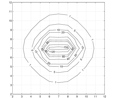
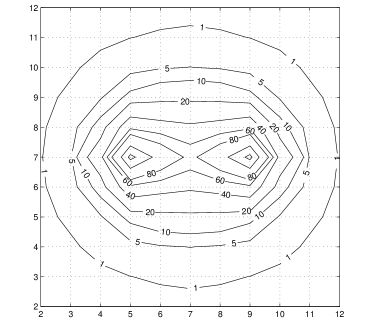
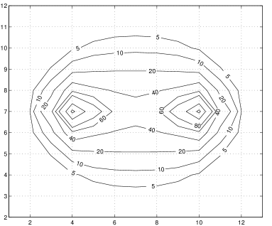
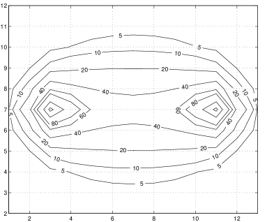
Figure 4: Two-quark action density at $T=3$ for a) $R=2$, b) $R=4$, c) $R=6$ and d) $R=8$. The units of isosurfaces are GeV/fm³.

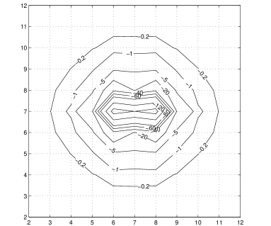
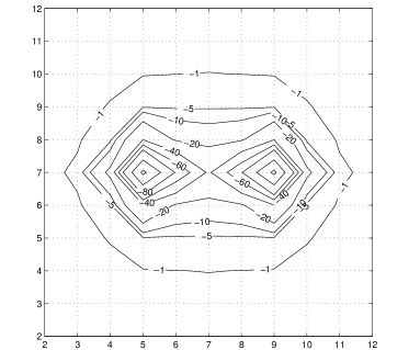
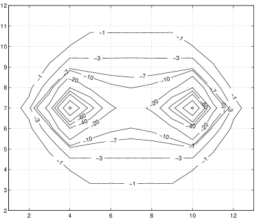
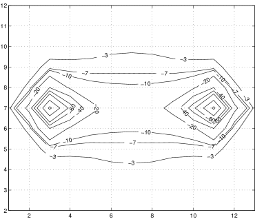
Figure 5: As in Fig. 4 but for the energy density (as in Eq. 14)

In these figures several points should be noted:

1) Both in the action and energy a flux tube structure clearly emerges as $R$ increases.

2) The action density is that given in Eq. 4 and is positive. However, for historical reasons, it is the ”negative” of the energy density that is plotted throughout this paper i.e. $\sum(S{\cal E}+U{\cal B})$ in the notations of Eq. 5 and 14.

3) At any given point, the magnitude of the energy field is a factor of about four less than that for the action.

4) The attractive potential between two quarks is responsible for the contours about a given quark being deformed. It is seen that these contours are more spread out in the direction of the second quark.

It should be added that all of these features are well known and can be found in Refs. [2, 10, 12]. The reason for repeating them here is to enable a comparison to be made with the four quark case to be discussed next.

5.2 Four quarks – before subtraction

We cut two-dimensional slices through the four-quark color field distributions to illuminate details. Let us first concentrate on the four-quark flux-distributions before any two-body contributions are subtracted from them. In Fig. 6 this is carried out for four quarks in the plane on which they lie. In Fig. 7 we look at the plane perpendicular to the one on which the quarks lie and cutting through the middle of the flux tubes along the sides. In Fig. 8 the plane is also perpendicular to the quark plane, but now cuts diagonally through two of the quarks. Figs. 9, 10, 11 show the same slices but for the energy distribution (as in Eq. 14). The $R=8$ data is taken in these three figures at $T=2$ because of a lack of signal at $T=3$.

Several points should be noted in these figures:

1) In Figs. 6 and 9 the self-actions and -energies in the neighborhoods of the four quarks clearly stand out, with the values at the actual positions of the quarks being given in Table 9, where they are compared with the corresponding two quark cases.

	$R=2$	4	6	8
4q action	0.0659(1)	0.0637(2)	0.0634(4)	0.0638(6)
energy	–0.0708(2)	–0.0680(4)	–0.0677(6)	–0.0684(9)
2q action	0.0652(1)	0.0639(1)	0.0635(1)	0.0634(2)
energy	–0.0718(1)	–0.0684(2)	–0.0679(2)	–0.0680(3)

Table 9: Self-energy peaks measured for two and four quarks at $T=2$. “Energy” refers to the combination in Eq. 14. The values are in lattice units.

2) As expected, most of the action and energy are contained in the area defined by the positions of the four quarks. This effect seems more pronounced as the sizes of the squares increase.

3) In Figs. 7 and 10 the flux tube profiles are seen to be distorted from that of two two-quark flux tubes. Furthermore, the distortion is such that the contours between the sides are more spread out than those outside the square. As mentioned in Sect. 5.1 a similar effect occurs with two quarks. This is a consequence of the additional attraction that arises when two two-quark flux tubes are brought together. As seen in Fig. 7, this attraction becomes very weak for $R\geq 8$, since then the flux tubes are essentially those of two independent flux tubes i.e. rotational invariance about their axes has been restored.

4) Figs. 8 and 11 show the self-actions and -energies at the end of the diagonals – the features are similar to those already seen in Figs. 7 and 10.

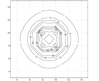
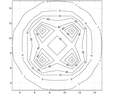
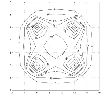
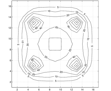
Figure 6: Four-quark action density at $T=3$ in the plane where the quarks lie for a) $R=2$, b) $R=4$, c) $R=6$ and d) $R=8$.

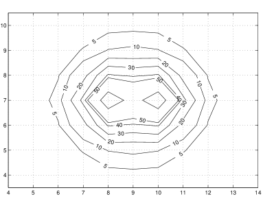
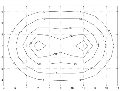
Figure 7: As in Fig. 6 but in the plane transverse to the quarks and in the middle of them.

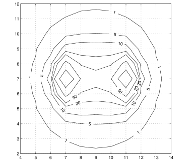
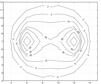
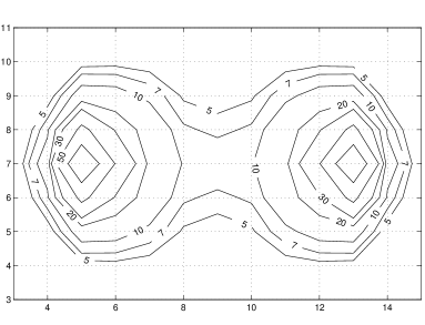
Figure 8: As in Fig. 6 but in the plane transverse to the quarks and cutting diagonally through them.

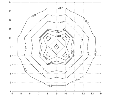
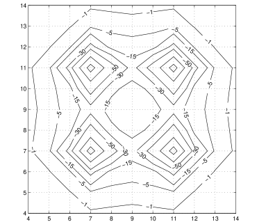
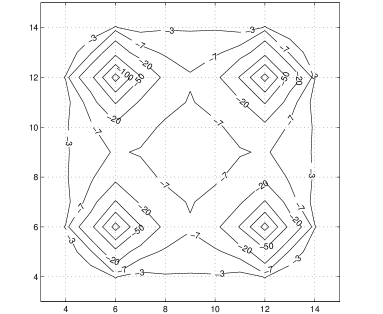
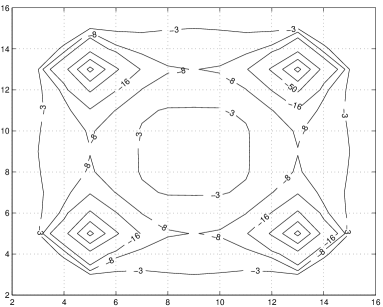
Figure 9: As in Fig. 6 but for the energy.

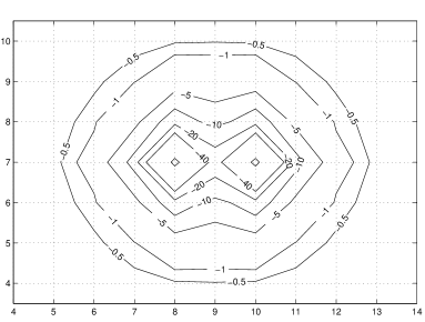
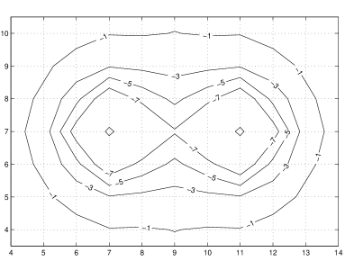
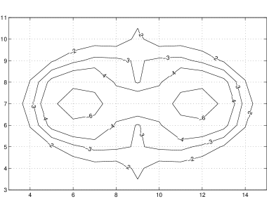
Figure 10: As in Fig. 7 but for the energy.

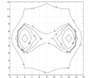
Figure 11: As in Fig. 8 but for the energy.

5.3 Four quarks – after subtraction

For a square of side $R$ the total four-quark energies $[E(4)]$ corresponding to Figs. 9–11 can be viewed as a combination of two terms:
1) The energy $E(AB)$ of two independent two-quark flux tubes of length $R$. This is simply $0.5[E(A)+E(B)]$ – due to the symmetry between the two partitions $A$ and $B$ depicted in Fig. 3.

2) The energy $[B(4)]$ binding the two two-quark systems i.e. $E(4)=E(AB)+B(4)$.

In practice $B(4)$ is only a few percent of $E(AB)$ as seen in Table 10.

	$R=2$	4	6	8
$E(4)$	1.069(1)	1.511(1)	1.861(4)	2.242(3)
$E(AB)$	1.127(1)	1.566(1)	1.891(2)	2.259(3)
$B(4)$	–0.058(1)	–0.055(3)	–0.030(1)	–0.017(1)

Table 10: Comparison of four-quark total and binding energies

Since energies are related to the profiles through Eq. 14 it is, therefore, natural to also view the flux tube energy profile $F(4)$ in Figs. 9–11 as being a combination of two terms $F(AB)+FB(4)$, where $F(AB)=0.5[F(A)+F(B)]$ is the average of the energy profiles for states $A$ and $B$ in Fig. 3. In other words, after subtracting the energy component of the two-body flux distributions $F(AB)$ of the two-body pairings, we get the distribution $FB(4)$, which can be considered as corresponding to the binding energy of the four quarks. The hope is that the form of $FB(4)$ will serve as a guide when constructing the type of model to be discussed in Sect. 6 – a model that only depends on the quark degrees of freedom. For the action there is no clear meaning to this subtraction, and so the action plots in this subsection are of an exploratory nature and will be compared to the energy plots to see what similarities exist.

Analogously to the unsubtracted case, Figs. 12–14 show the action densities for the three slices, while the energy densities are plotted in Figs. 15–17. Being guided by the sum rules in Table 6, the energy densities are taken at $T=2$ for $R=4,6$ and at $T=3$ for $R=2$.

As expected, there is again a large cancellation between $F(AB)$ and $F(4)$. However, as seen from Table 9, the dominant feature in both $F(4)$ and $F(AB)$ – the self-energies – are equal to within less than 1%. For the $R=2$ case the agreement in the table is worse, as the four-quark binding signal extends in this small system to the quark positions – as seen in Figs. 15–17. Therefore, the residual profile $FB(4)$ is expected to have a realistic signal not dominated by self-energy cancellation errors. This is seen in Fig. 15, where there is no particular structure at the positions of the four quarks. Elsewhere, $F(4)$ and $F(AB)$ cancel to leave $|FB(4)|\approx|F(AB)|/10$ over the area defined by the four quarks. In spite of this delicate cancellation, $FB(4)$ is seen to be everywhere positive for all the $R$’s considered. Therefore, due to our sign convention, $FB(4)$ represents a negative energy density – as expected for a bound state.

It is of interest to see in detail the contributions to $FB(4)$ from the five terms $F(4)$ and $F(AB)=0.5[F(12)+F(34)+F(13)+F(24)]$. These are given in Table 11 for three different points in the plane of the quarks. Here it is seen that at point (b) – in the middle of the line connecting quarks 1 and 2 – the cancellation is a complicated procedure with the resulting attraction arising from the combined effect of flux tubes (12), (13) and (24). The effect from (12) alone is not enough to overcome the signal in the four-quark distribution.

Position	$F(4)$	$0.5F(12)$	$0.5F(34)$	$0.5F(13)$	$0.5F(24)$	$FB(4)$
(a)	–0.00262(4)	–0.00076(1)	–0.00076(1)	–0.00076(1)	–0.00076(1)	0.00043(3)
(b)	–0.00834(3)	–0.00778(3)	–0.00002(1)	–0.00076(1)	–0.00076(1)	0.00098(2)
(c)	–0.06797(34)	–0.03420(8)	–0.00002(1)	–0.03420(8)	–0.00002(1)	0.00047(26)

Table 11: The contributions to $FB(4)$ at three points in the plane of the square with side $R=4$ (here the $T=2$ data is used). The positions are (a) – the center of the square, (b) – the middle of (12), (c) – at quark 1.

In Figs. 15–17, $FB(4)$ has a roughly spherical shape for $R=2$, with the shape getting more elongated when viewed from the side of the quark plane as in Fig. 16. For $R=4$ we observe a clear region of binding in between the quarks. In Fig. 15 b) it has the shape of a regular octagon bounded by the quarks, that extends outside the quark square in between two nearest neighbor quarks. In the latter region we can see maxima (with errors of 2–20%) that resemble the two-body flux-tubes. This is understandable as in the four-quark distributions before subtraction we observed that the fields were pulled towards the centerpoint, leaving a smaller contribution in the middle of the sides of the square. Therefore, when the two-body distributions are subtracted we are left with larger positive (binding in our sign convention) contributions at these points. The region inside the quark square has a constant density and thickness, except when viewed diagonally in Fig. 17 b), where the maxima at the sides do not contribute. A qualitatively similar situation is observed for $R=6$, with more contribution in the maxima at the sides and less in between them. An area of constant thickness in between the sides of the square can still be observed in Fig. 16 c). The drop in action density right at the center observed in Figs. 15 c), 16 c) can be at least partly attributed to the poor performance of our variational basis for this $R$ value at the center point as discussed in Sect. 2.2. With a better basis we would expect the hole in the center of Fig. 16 c) to disappear and Fig. 15 c) to have more contribution in the place of the valley in the center.

The exploratory plots for the action in Figs. 12–14 show a more complicated structure than the corresponding ones for the energy. For $R=4,6$ there is an area of negative (“binding”) density around the center, where the distribution has a positive sign. Positive contributions are also found outside the corners of the square. For $R=6$ the negative area is broken into four separate pieces. These complicated action distributions are in sharp contrast to the the simple connected regularity of the binding distributions in the energy case. This fits in with the clear physical interpretation of the energy distributions in this subtracted case, unlike the ones for the action.

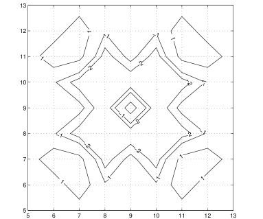
Figure 12: As in Fig. 6 but after subtracting two-body tubes along the sides.

Figure 13: As in Fig. 7 but after subtraction.

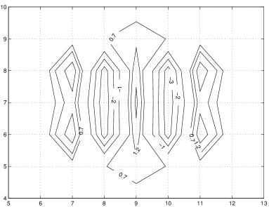
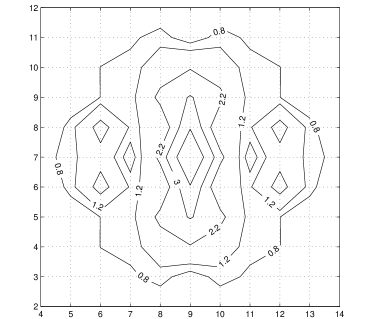
Figure 14: As in Fig. 8 but after subtraction.

Figure 15: As in Fig. 12 but for the energy – called $FB(4)$ in the text.

Figure 16: As in Fig. 13 but for the energy.

Figure 17: As in Fig. 14 but for the energy.

5.4 First excited state

The first excited state of four quarks is not bound, and its wavefunction is close to $(|A\rangle-|B\rangle)/\sqrt{2}$ both when two or three basis states are considered.

The energy distribution of this state is presented in Fig. 18 for $R=2,4$. These are taken at $T=3,2$ respectively, being again guided by Tables 4 and 6. Very little difference compared with the ground state pictures in Fig. 9 can be seen. However, after the ground-state two-body flux tubes are subtracted, a very different picture emerges – as seen in Figs. 19–21. The large negative contributions (due to our sign convention) in these three figures are evidence of the unbound nature of the state. Comparison of Figs. 19 and Fig. 15 shows clearly the different symmetry in this case; for the ground state a roughly spherical distribution is found with concentrated areas at the sides of the square, whereas for the excited state the distribution is concentrated in the corners of the square near the quarks and decreased at the middle of the sides, showing a cloverleaf-shaped structure. For $R=4$ the negative distribution is concentrated in the center with remnants outside the sides of the square, with a positive “cloverleaf” in between these regions, indicating a node in the wavefunction of the excited state. In Figs. 20 and 21 the distribution can be seen to have a larger extent outside the quark plane than the ground state.

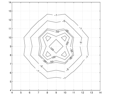
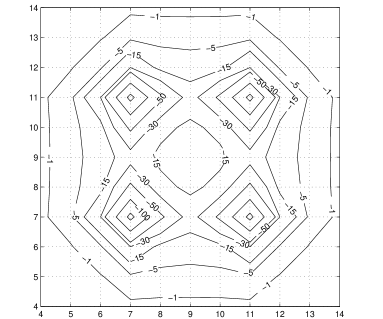
Figure 18: As in Fig. 9 but for the first excited state and $R=2,4$.

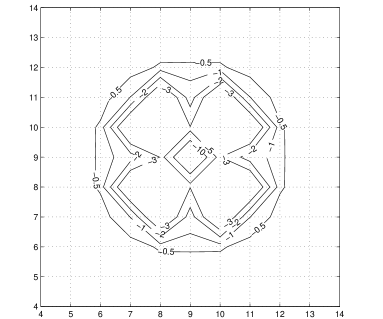
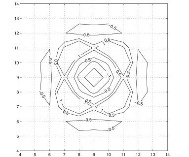
Figure 19: As in Fig. 15 but for the first excited state.

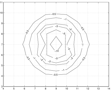
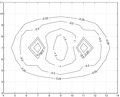
Figure 20: As in Fig. 16 but for the first excited state.

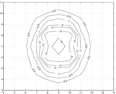
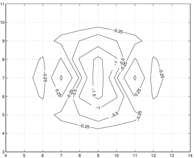
Figure 21: As in Fig. 17 but for the first excited state.

5.5 Chromomagnetic fields

As discussed in Sect. 2.1, we measure separately the spatial components of chromoelectric and -magnetic fields. However, full information on the direction of these fields is not available, as the measured quantities correspond to the squares of the components. Therefore the pictures in this section have been created by inserting the signs of the components by hand.

In Fig. 22 for two quarks the magnetic field in the plane perpendicular to the interquark axis and in the middle of the quarks is shown. The signs have been chosen so that the magnetic field rotates around a flux-tube. In Fig. 23 the magnetic field is shown for the four-quark case in the plane perpendicular to the quark plane and cutting through the middle as in Fig. 7. Comparison between Figs. 22 and 23 shows how the two-quark fields get distorted in the four-quark case – an effect already seen in earlier figures. The field in the middle of the four quarks can be seen to have a direction more perpendicular to the quark plane in the $R=8$ case than for $R=4$.

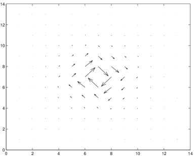
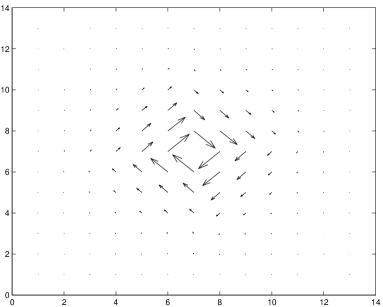
Figure 22: Magnetic field in the transverse plane in the middle of two quarks at separation a) $R=4$ and b) $R=8$.

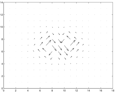
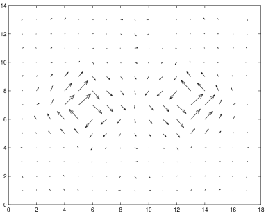
Figure 23: Magnetic field in the transverse plane in the middle of four quarks at separation a) $R=4$ and b) $R=8$.

6 Overlap of fluxes and a model for the energies

A simple version of the binding energy model in Ref. [16] using only two basis states (A,B) reproduces well the observed ground and excited state binding energies of four quarks at the corners of a square. Therefore it is interesting to see how the observed flux distributions corresponding to the binding energy relate to the model.

The two-state version of the model gives the energies as eigenvalues $E(4)$ of

$$\left[{\bf V}-E(4){\bf N}\right]=0,$$ (18)

where

$${\bf N}=\left(\begin{array}[]{ll}1&-f/N\\ -f/N&1\end{array}\right)\ \ {\rm and}\ \ {\bf V}=\left(\begin{array}[]{cc}v_{13}+v_{24}&\frac{f}{N}V_{AB}\\ \frac{f}{N}V_{BA}&v_{14}+v_{23}\end{array}\right),$$ (19)

and $v_{ij}$ are the static two-body potentials between quarks $i$ and $j$. The matrix element $V_{AB}$ ($=V_{BA}$) comes from the perturbative expression

$$V_{ij}=-\frac{1}{N^{2}-1}{\bf T_{i}}\cdot{\bf T_{j}}v_{ij}=-\left(v_{13}+v_{24}+v_{14}+v_{23}-v_{12}-v_{34}\right),$$ (20)

where for a color singlet state $[ij]^{0}$ the normalization is chosen to give
$\langle[ij]^{0}|V_{ij}|[ij]^{0}\rangle=v_{ij}$. The four-quark binding energies $B(4)$ are obtained by subtracting the internal energy of the basis state with the lowest energy, e.g.

$$B(4)=E(4)-(v_{13}+v_{24}).$$

In our case we take them from Table 10.

A central element in this model is the phenomenological factor $f$ appearing in the overlap of the basis states $\langle A|B\rangle=-f/N$ for $SU(N_{c})$. This factor is a function of the spatial coordinates of all four quarks, making the off-diagonal elements of ${\bf V}$ in Eq. 19 four-body potentials. It attempts to take into account the decrease of overlap from the weak coupling limit, where $\langle A|B\rangle=-1/N$, to the strong coupling limit where $\langle A|B\rangle=0$. Perturbation theory to $O(\alpha^{2})$ also produces the two-state model of Eqs. 18–20 with $f=1$ [17]. A working parameterization for $f$ is

$$f=e^{-k_{A}b_{S}A-k_{P}\sqrt{b_{S}}P}.$$ (21)

Here $b_{S}$ is the string tension and $k_{A},k_{P}$ parameters multiplying, respectively, the minimal area and its perimeter bounded by the four quarks. In a fit to energies of square and tilted rectangle geometries at $\beta=2.4$ in Ref. [5] the values of these parameters were $k_{A}=0.38(4),\;k_{P}=0.087(10)$. In a continuum extrapolation the $k_{A}$ increased to a value close to one and $k_{P}$ approached zero. Also in Ref. [7] a fit to many additional geometries, but with $k_{P}$ fixed at zero, yielded $k_{A}=0.57(1)$.

With this model, the ground state energy for a square geometry is

$$B(4)=\frac{f}{1+f/2}(v_{s}-v_{d}),$$ (22)

giving

$$f=\frac{B(4)}{v_{s}-v_{d}}(1-\frac{1}{2}\frac{B(4)}{v_{s}-v_{d}})^{-1}.$$ (23)

Here $v_{s},v_{d}$ are the two-body potentials $v_{ij}$ between quarks on one side and in the opposite corners of the square, respectively. This leads to the values of $f$ shown in Table 12. The expression in Eq. 22 can now be rewritten in terms of the sums over the corresponding field distributions $\sum F$ in Eq. 14 as

$$\sum FB(4)=\frac{f}{1+f/2}\sum\frac{1}{2}[F(AB)-F(C)]$$ (24)

Of course, if the sum rules were satisfied exactly, then this equation would add nothing new to our knowledge of $f$. However, as seen in Table 6 the errors on some of the sums can be quite large. Therefore, if Eq. 24 is used to extract $f$ values, the resultant numbers are found to be only meaningful for the $R=2$ case – as seen in Table 12.

Our original hope when embarking on this aspect of the study was that a comparison could be made between the integrands in Eq. 24, in order to say more about the form of $f$. However, this has had only limited success. The outcome is summarized in Figs. 24 and 25. Figure 24 shows the microscopic distribution of $FB(4)$ and $F(AB)-F(C)$, measured at the center point in between the four quarks and moving away a) along the quark plane through the flux tube in between two quarks or b) up in the direction normal to the plane of the quarks. Figure 25 shows the ratio $2FB(4)/[F(AB)-F(C)]$ on these same axes; the ratio $2FB(4)/[F(AB)-F(C)]/(1-FB(4)/[F(AB)-F(C)])$ which is analogous to Eq. 23, but involves the integrands instead of the integrals in Eq. 24, has similar profiles (not shown).

Figure 24: $FB(4)$ and $0.5[F(AB)-F(C)]$ away from the center point – a) on the quark plane for $R=2,4,6\;$ – b) moving up from the quark plane. The $R=2$ data is taken at $T=3$ and the $R=4,6$ data at $T=2$.

Figure 25: The ratio $2FB(4)/[F(AB)-F(C)]$ on the same axis as in Fig. 24.

In Figs. 24 a,b) it is seen that the $0.5[F(AB)-F(C)]$ profile drops away more rapidly than that for $FB(4)$. Therefore, if $-f/(1+0.5f)$ is interpreted as a form factor acting on the basic two-body profiles, it should not have a spatial extent larger than the profile it is modifying. This interpretation should become clearer for the larger values of $R$, where lattice artefacts play less of a role. Looking at $R=4,6$ it is seen that $0.5[F(AB)-F(C)]$, in fact, drops by almost an order of magnitude on reaching the side of the square. Therefore the ”extent” of $0.5[F(AB)-F(C)]$ is less than $R\times R$ – being more like $(R-1)\times(R-1)$. This suggests that the ”extent” of $-f/(1+0.5f)$ and, likewise, $f$ should have the same limit. Consequently, when $f$ is parametrized as in Eq. 21, it could be more realistic to use, in place of the area $A=R^{2}$ contained by the four quarks, an effective area that is somewhat less. This interpretation fits in with the value of $k_{A}<1$ in Eq. 21 obtained in Ref. [5]. In the continuum limit, however, $k_{A}$ was there found to approach one.

An alternative view that is more in line with the interpretation that $f$ is a form factor is to rewrite Eq. 21 as $f=\exp(-A/A_{\rm effective})$, where $A_{\rm effective}=(k_{A}b_{S})^{-1}$. Here the perimeter term has been forgotten. For the case of squares a sensible definition of ”range” is then $R_{\rm effective}=\sqrt{A_{\rm effective}}$. As stated after Eq. 21, in Ref. [7] for the two basis state model the value of $k_{A}$ is 0.57(1) giving $R_{\rm effective}=5.0$.

$R$	type	$T=2$	$T=3$	$T=4$
2	energy	0.7393(26)	0.7586(33)	0.7635(39)
	sum 1	0.69(12)	0.63(16)	0.56(21)
	sum 2	0.70(13)	0.59(17)	0.55(25)
4	energy	0.4760(23)	0.4688(36)	0.4655(56)
	sum 1	0.9(2.7)
	sum 2	0.9(3.9)	0.39(33)
6	energy	0.1504(61)	0.1931(81)	0.190(24)
	sum 1	0.42(81)
8	energy	0.0373(22)	0.0541(91)	0.048(48)

Table 12: The value of $f$ from energies and energy sums

However, the main weakness in the above comparison of integrands is that, although the two basis state model ($A,B$ in Fig. 3) is able to give a good fit to much of the four-quark data in Ref. [4], it is unable to explain other data – in particular that of four quarks at the corners of a regular tetrahedron. In Refs. [6, 7] it is shown that a more successful model utilizes six basis states – $A,B,C$ in Fig. 1 and $A^{*},B^{*},C^{*}$ where each quark pair is now in an excited gluonic state. For this model the $A^{*},B^{*},C^{*}$ contribution begins to dominate as the interquark distances increase. For example, with $\beta=2.4$ the $A,B,C$ component contributes only 40% (10%) to the binding energy of four quarks at the corners of a square with sides $R=4(6)$. Another feature of this extended version is that $k_{A}$ in Eq. 21 becomes 1.51(8), giving $R_{\rm effective}=3.1$. This implies that the longer range in the two basis state model is merely simulating the effect of $A^{*},B^{*},C^{*}$ and that, when these three states are treated explicitly, the basic interaction containing $f$ is of shorter range. But it is beyond the scope of the present study to pursue this further, since it requires ingredients that are not available from the present calculation – in particular for two quarks the profiles of fields where the glue is in an excited state with $E_{u}$ symmetry.

7 Conclusions

We have measured the full flux distributions of two quarks and four quarks at the corners of a square in quenched SU(2) lattice gauge theory with $\beta=2.4$ on a $20^{3}\times 32$ lattice. Multihit variance reduction was used to improve the signal on temporal links and switched off at the quark lines for proper measurement of self-energies. The effect from the multihit was helpful, but not as dramatic as expected. Using values of generalized $\beta$-functions from Ref. [2] we were able to use lattice sum rules, giving either the observed energy or zero, to see where the measurements were expected to be most accurate. This strategy was particularly useful after self-energies were removed by subtracting two distributions, and enabled us to choose the best data to analyse.

The four-quark distributions in Figs. 6–11 show how the interaction pulls the distribution to the middle of the quarks. This effect decreases when the quarks move further apart.

The distributions corresponding to the binding energies of the quarks, obtained by subtracting the distributions of the lowest-lying two-quark pairings from the four quark one, are shown in Figs. 15–17. They can be seen to form a “cushion” of approximately constant density and height in between the quarks with tubes of larger density in between nearest neighbor quarks.

For the first excited state of the four quarks we observe – after subtraction – an energy field structure that is much more complicated (Fig. 19) than that for the ground state (Fig. 15). This presumably arises because the states $A$ and $B$ are basically combined as $A+B$ in the ground state and $A-B$ in the excited state, the latter leading naturally to cancellations. As a general statement it is seen that the energy profiles in Figs. 15–21 show an increasing amount of fine detail – all of which is ’real’ in the sense of being larger than the statistical errors. This data is a real challenge for any model that claims to simulate the original gauge field theory. Unfortunately, at present, such theories are in their infancy. For example, the dual model of Ref. [18] has had some success in describing – for two quarks – the energy profile for the gluon field in its ground state. However, so far it has been unable to say anything about four quarks or excited gluon fields in the two-quark case.

Our original hope was that these residual fields would give some guidance when constructing models that are explicitly dependent only on the quark positions. In the case of the model presented in Sect. 6 the main conclusion was that the model was seen to be qualitatively consistent with the data. The data was unable to say anything about the actual form of the multi-quark interaction term $f$ in Eq. 21 besides the fact that it should be contained inside the area of the four quarks – suggesting an effective interaction area somewhat smaller than the full $R^{2}$ area of the square. Such a smaller area is consistent with our earlier fit results. However, only when the six basis state model has replaced the two basis state analysis of Section 6 can more definite statements be made.

Apart from this paper, we are not aware of any theoretical attempts to understand the four-quark flux distribution. Hopefully the data presented here will be useful for such attempts.

8 Acknowledgement

The authors wish to thank P. Kurvinen for developing much of the analysis code. Funding from the Finnish Academy and M. Ehrnrooth foundation (P.P) is gratefully acknowledged. Our simulations were performed on the Cray C94 at the Center for Scientific Computing (CSC) in Espoo. We thank M. Gr hn from CSC for help in visualizing the color fields.

References

- [1] A. M. Green, C. Michael and P. S. Spencer, Phys. Rev. D55 1216 (1997), hep-lat/9610011.
- [2] P. Pennanen, A. M. Green and C. Michael, Phys. Rev. D56 3903–3916 (1997), hep-lat/9705033.
- [3] M. Teper, Phys. Lett. B397 223 (1997), hep-lat/9701003.
- [4] A. M. Green, J. Lukkarinen, P. Pennanen and C. Michael, Phys. Rev. D53 261–272 (1996), hep-lat/9508002.
- [5] P. Pennanen, Phys. Rev. D55 3958–3965 (1997), hep-lat/9608147.
- [6] A. M. Green and P. Pennanen, to be published in Phys. Lett. B (1998), HIP–1997–55 / TH, hep-lat/9709124.
- [7] A. M. Green and P. Pennanen, preprint HIP–1998–01 / TH (1998), hep-lat/9804003.
- [8] G. Parisi, R. Petronzio and F. Rapuano, Phys. Lett. 128B 418 (1983).
- [9] R. Brower and P. Rossi, Nucl. Phys. B 190, 699 (1981).
- [10] R. W. Haymaker, V. Singh, Y.-C. Peng and J. Wosiek, Phys. Rev. D53 389 (1996), hep-lat/9406021.
- [11] C. Michael, Nucl. Phys. B259, 58 (1985).
- [12] G. S. Bali, K. Schilling and C. Schlichter, Phys. Rev. D51 5165–5198 (1995), hep-lat/9409005.
- [13] C. Michael, A. M. Green and P. S. Spencer, Phys. Lett. B 386, 269 (1996).
- [14] C. Michael, Nucl. Phys. B 280, 13 (1987).
- [15] C. Michael, Phys. Rev. D53 4102–4105 (1996), hep-lat/9504016.
- [16] A. M. Green, C. Michael and J. E. Paton, Nucl. Phys. A554 701–720 (1993), hep-lat/9209019.
- [17] J. T. A. Lang, J. E. Paton and A. M. Green, Phys. Lett. B366 18–25 (1996), hep-ph/9508315.
- [18] M. Baker, J. S. Ball and F. Zachariasen, Int. J. Mod. Phys. A11, 343–360 (1996).