UTCCP-P-33 MPI-PhT/98-15 UTHEP-380 Perturbative Renormalization Factors of Bilinear Quark Operators for Improved Gluon and Quark Actions in Lattice QCD

Abstract

We calculate one-loop renormalization factors of bilinear quark operators for gluon action including six-link loops and $O(a)$-improved quark action in the limit of massless quark. We find that finite parts of one-loop coefficients of renormalization factors diminish monotonically as either of the coefficients $c_{1}$ or $c_{2}+c_{3}$ of the six-link terms are decreased below zero. Detailed numerical results are given, for general values of the clover coefficient, for the tree-level improved gluon action in the Symanzik approach $(c_{1}=-1/12,c_{2}=c_{3}=0)$ and for the choices suggested by Wilson $(c_{1}=-0.252,c_{2}=0,c_{3}=-0.17)$ and by Iwasaki $(c_{1}=-0.331,c_{2}=c_{3}=0$ and $c_{1}=-0.27,c_{2}+c_{3}=-0.04)$ from renormalization-group analyses. Compared with the case of the standard plaquette gluon action, finite parts of one-loop coefficients are reduced by 10–20% for the Symanzik action, and approximately by a factor two for the renormalization-group improved gluon actions.

I Introduction

Lattice QCD calculations of hadron matrix elements require values of renormalization factors which relate operators on the lattice to those in the continuum. For the standard plaquette gluon action, perturbative calculation of renormalization factors for massless quark has been carried out to one-loop order for bilinear and four-quark operators, both for the Wilson quark action[1, 2, 3, 4, 5, 6] and for the $O(a)$-improved “clover” action [7, 8, 9, 10, 11, 12] originally suggested by Sheikholeslami and Wohlert[13, 14]. With developments of our full QCD simulations[15] employing an improved gluon action[16], we find it necessary to extend these calculations. In this article we report results for renormalization factors of bilinear quark operators at the one-loop level for the gluon action improved by addition of six link loops to the plaquette term. For the quark action we treat both the Wilson and $O(a)$-improved actions, taking the limit of massless quark. We evaluate numerical values of the one-loop coefficients of renormalization factors for the case of tree-level improved action in the Symanzik approach[17, 18], and for several cases of renormalization-group improved actions[16, 19]. We also examine how the one-loop coefficients vary for general values of the coefficients of the six-link loop terms.

In Sec. II we write down the action we treat and the Feynman rule to fix our conventions. The structure of renormalization factors related to fermion self-energy is discussed in Sec. III, and that for bilinear quark operators in Sec. VI. Numerical results for one-loop coefficients are given in Sec. V. Since the procedure of calculation is by now standard, we shall be brief on this point. Expressions for one-loop integrands are listed in Appendix A. In Appendix B we collect one-loop results for the relation between the renormalized and bare coupling constants for various choices of gluon and quark actions.

II Action and Feynman rule

The gluon action we consider is defined by

$$S_{\rm gluon}=\frac{1}{g^{2}}\left\{c_{0}\sum_{plaquette}{\rm Tr}U_{pl}+c_{1}\sum_{rectangle}{\rm Tr}U_{rtg}+c_{2}\sum_{chair}{\rm Tr}U_{chr}+c_{3}\sum_{parallelogram}{\rm Tr}U_{plg}\right\},$$ (1)

where the first term represents the standard plaquette term, and the remaining terms are six-link loops formed by a $1\times 2$ rectangle, a bent $1\times 2$ rectangle (chair) and a 3-dimensional parallelogram. The coefficients $c_{0},\cdots,c_{3}$ satisfy the normalization condition

$$c_{0}+8c_{1}+16c_{2}+8c_{3}=1.$$ (2)

For the quark action we consider

$$S_{\rm quark}=S_{\rm W}+S_{\rm C},$$ (3)

where $S_{\rm W}$ is the Wilson action given by

$$S_{\rm W}=a^{3}\sum_{n}\frac{1}{2}\sum_{\mu}\left(\overline{\psi}_{n}(-r+\gamma_{\mu})U_{n,\mu}\psi_{n+\hat{\mu}}+\overline{\psi}_{n}(-r-\gamma_{\mu})U^{\dagger}_{n-\mu,\mu}\psi_{n-\hat{\mu}}\right)+(am_{0}+4r)\overline{\psi}_{n}\psi_{n}$$ (4)

with $a$ the lattice spacing, and $S_{\rm C}$ represents the “clover” term defined by

$$S_{\rm C}=-c_{\rm SW}a^{3}\sum_{n}\sum_{\mu,\nu}ig\frac{r}{4}\overline{\psi}_{n}\sigma_{\mu\nu}P_{\mu\nu}(n)\psi_{n}.$$ (5)

For the field strength $P_{\mu\nu}$ we adopt the definition given by

$$P_{\mu\nu}(n)=\frac{1}{4}\sum_{i=1}^{4}\frac{1}{2ig}\left(U_{i}(n)-U^{\dagger}_{i}(n)\right),$$ (6)

$$U_{1}(n)=U_{n,\mu}U_{n+\hat{\mu},\nu}U^{\dagger}_{n+\hat{\nu},\mu}U^{\dagger}_{n,\nu},$$ (7)

$$U_{2}(n)=U_{n,\nu}U^{\dagger}_{n-\hat{\mu}+\hat{\nu},\mu}U^{\dagger}_{n-\hat{\mu},\nu}U_{n-\hat{\mu},\mu},$$ (8)

$$U_{3}(n)=U^{\dagger}_{n-\hat{\mu},\mu}U^{\dagger}_{n-\hat{\mu}-\hat{\nu},\nu}U_{n-\hat{\mu}-\hat{\nu},\mu}U_{n-\hat{\nu},\nu},$$ (9)

$$U_{4}(n)=U^{\dagger}_{n-\hat{\nu},\nu}U_{n-\hat{\nu},\mu}U_{n+\hat{\mu}-\hat{\nu},\nu}U^{\dagger}_{n,\mu}.$$ (10)

Our $\gamma$ matrix convention is as follows:

$$\gamma_{i}=\pmatrix{0&-i\sigma^{i}\cr i\sigma^{i}&0\cr},\quad\gamma_{4}=\pmatrix{0&1\cr 1&0\cr},$$ (11)

$$\gamma_{5}\equiv\gamma_{1}\gamma_{2}\gamma_{3}\gamma_{4}=\pmatrix{1&0\cr 0&-1\cr},$$ (12)

$$\sigma_{\mu\nu}=\frac{1}{2}\left[\gamma_{\mu},\gamma_{\nu}\right].$$ (13)

Weak-coupling perturbation theory is developed by writing

$$U_{n,\mu}=\exp(igaA_{\mu}(n+\frac{1}{2}\hat{\mu})).$$ (14)

We adopt a covariant gauge fixing with a gauge parameter $\alpha$ defined by

$$S_{\rm GF}=a^{4}\sum_{n}\frac{1}{2\alpha}\left(\nabla_{\mu}A_{\mu}^{a}(n+\frac{1}{2}\hat{\mu})\right)^{2},$$ (15)

where $\nabla_{\mu}f_{n}\equiv(f_{n+\hat{\mu}}-f_{n})/a$. The free part of the gluon action takes the form

$$S_{0}=\frac{1}{2}\int_{-\pi/a}^{+\pi/a}\frac{d^{4}k}{(2\pi)^{4}}\sum_{\mu,\nu}A_{\mu}^{a}(k)G_{\mu\nu}A_{\nu}^{a}(-k),$$ (16)

where

$$G_{\mu\nu}=\hat{k}_{\mu}\hat{k}_{\nu}+\sum_{\rho}(\hat{k}_{\rho}\delta_{\mu\nu}-\hat{k}_{\mu}\delta_{\rho\nu})q_{\mu\rho}\hat{k}_{\rho}$$ (17)

with

$$\hat{k}_{\mu}=\frac{2}{a}\sin\frac{k_{\mu}a}{2}$$ (18)

and $q_{\mu\nu}$ is defined as

$$q_{\mu\nu}=(1-\delta_{\mu\nu})\left(1-(c_{1}-c_{2}-c_{3})a^{2}(\hat{k}_{\mu}^{2}+\hat{k}_{\nu}^{2})-(c_{2}+c_{3})a^{2}\hat{k}^{2}\right).$$ (19)

The gluon propagator can be written as

$$D_{\mu\nu} = (\hat{k}^{2})^{-2}\left[\hat{k}_{\mu}\hat{k}_{\nu}+\sum_{\sigma}(\hat{k}_{\sigma}\delta_{\mu\nu}-\hat{k}_{\nu}\delta_{\mu\sigma})\hat{k}_{\sigma}A_{\sigma\nu}\right]-(1-\alpha)\frac{\hat{k}_{\mu}\hat{k}_{\nu}}{(\hat{k}^{2})^{2}}$$ (20)

$$= (\hat{k}^{2})^{-2}\left[(1-A_{\mu\nu})\hat{k}_{\mu}\hat{k}_{\nu}+\delta_{\mu\nu}\sum_{\sigma}\hat{k}_{\sigma}^{2}A_{\nu\sigma}\right]-(1-\alpha)\frac{\hat{k}_{\mu}\hat{k}_{\nu}}{(\hat{k}^{2})^{2}},$$ (21)

where $A_{\mu\nu}$ is a function of $q_{\mu\nu}$ and $\hat{k}_{\mu}$ whose form we refer to the original literatures[16, 17].

The free quark propagator is given by

$$S_{\rm q}(p)=\frac{-i\sum_{\mu}\gamma_{\mu}\overline{p}_{\mu}+W(p)}{\sum_{\mu}\overline{p}_{\mu}^{2}+W(p)^{2}},$$ (22)

where

$$\bar{k}_{\mu} = \frac{1}{a}\sin k_{\mu}a$$ (23)

$$W(p) = m+\frac{r}{a}\sum_{\mu}(1-\cos ap_{\mu}).$$ (24)

To calculate renormalization factors of bilinear quark operators to one-loop order, we need only one- and two-gluon vertices with quarks. The vertices originating from the Wilson quark action are given by

$$V_{1\mu}^{a}(k,p) = -igT^{a}\{\gamma_{\mu}\cos\frac{a}{2}(-k_{\mu}+p_{\mu})-ir\sin\frac{a}{2}(-k_{\mu}+p_{\mu})\},$$ (25)

$$V_{2\mu\nu}^{ab}(k,p) = \frac{a}{2}g^{2}\frac{1}{2}\{T^{a},T^{b}\}\{i\gamma_{\mu}\sin\frac{a}{2}(-k_{\mu}+p_{\mu})-r\cos\frac{a}{2}(-k_{\mu}+p_{\mu})\}\delta_{\mu\nu},$$ (26)

and the interaction due to the clover term has the form

$$V_{{\rm C}1\mu}^{a}(k,p)=-c_{\rm SW}g\frac{r}{2}\left(\sum_{\nu}\sigma_{\mu\nu}\sin a(p_{\nu}+k_{\nu})\right)\cos\frac{a}{2}(p_{\mu}+k_{\mu})T^{a}.$$ (27)

Our momentum assignments for the vertices are depicted in Fig. 1. The two-gluon vertex with quarks from the clover term gives no contribution to diagrams we evaluate, and is hence omitted.

III Quark serf-energy

Let us write the inverse full quark propagator as

$$S_{\rm q}^{-1}(p)=i\gamma_{\mu}\bar{p}_{\mu}+W(p)-\Sigma(p).$$ (28)

Calculating the quark self-energy $\Sigma(p)$ to one-loop order on the lattice and making an expansion of form

$$\Sigma(p)=\Sigma(0)+\frac{\partial\Sigma(0)}{\partial p_{\mu}}p_{\mu}+O(p^{2}),$$ (29)

we find

$$S_{q}^{-1}(p) = i\gamma_{\mu}p_{\mu}\left[1-\frac{g^{2}}{16\pi^{2}}C_{F}\left\{\log(\lambda a)^{2}+\Sigma_{1}+(\alpha-1)(\log(\lambda a)^{2}+\Sigma_{\alpha})\right\}\right]$$ (31)

$$+m\left[1-\frac{g^{2}}{16\pi^{2}}C_{F}\left\{4\log(\lambda a)^{2}+\Sigma_{2}+(\alpha-1)(\log(\lambda a)^{2}+\Sigma_{\alpha})\right\}\right],$$

where

$$m=m_{0}-\frac{g^{2}}{16\pi^{2}}C_{F}\frac{\Sigma_{0}}{a}.$$ (32)

In (31) the coefficients of $i\gamma_{\mu}p_{\mu}$ and $m$ are evaluated with $m_{0}=0$. The infrared divergence that appears in this case is regularized by a gluon mass $\lambda$ introduced in the gluon propagator as described in Appendix A. Of the finite constants $\Sigma_{i}(i=0,1,2,\alpha)$, $\Sigma_{\alpha}$ is independent of the clover coefficient $c_{SW}$ nor does it depend on the improved part of the gluon action. The other constants $\Sigma_{i}(i=0,1,2)$ depend quadratically on the clover coefficient $c_{SW}$, and we write

$$\Sigma_{i} = \Sigma_{i}^{(0)}+c_{SW}\Sigma_{i}^{(1)}+c_{SW}^{2}\Sigma_{i}^{(2)}.$$ (33)

Let us recall that the hopping parameter $K$ is related to the bare quark mass $m_{0}$ through

$$K=\frac{1}{2(m_{0}a+4)}$$ (34)

The critical hopping parameter corresponding to massless quark is given by

$$K_{c}=\frac{1}{8}\left(1-\frac{g^{2}}{16\pi^{2}}C_{F}\frac{\Sigma_{0}}{4}\right).$$ (35)

In the continuum we employ the $\overline{MS}$ scheme with naive dimensional regularization. The one-loop self-energy in the continuum has the same form as (31) with, however, the replacements,

$$\log(\lambda a)^{2} \to \log(\lambda/\mu)^{2},$$ (36)

$$\Sigma_{1} \to \Sigma_{1}^{\overline{MS}}=1/2,$$ (37)

$$\Sigma_{2} \to \Sigma_{2}^{\overline{MS}}=-2,$$ (38)

$$\Sigma_{\alpha} \to \Sigma_{\alpha}^{\overline{MS}}=-1.$$ (39)

Let us define the quark wave function renormalization factor needed for converting the lattice field to the continuum field in the $\overline{MS}$ scheme by

$$\psi^{\overline{MS}}=Z_{\psi}\psi^{lat}.$$ (40)

To one-loop order we then find that

$$Z_{\psi}(\mu a)=1+\frac{g^{2}}{16\pi^{2}}C_{F}\left[-\log(\mu a)^{2}+z_{\psi}+(\alpha-1)(-\log(\mu a)^{2})\right].$$ (41)

where

$$z_{\psi}=\Sigma_{1}^{\overline{MS}}-\Sigma_{1}+(\alpha-1)(\Sigma_{\alpha}^{\overline{MS}}-\Sigma_{\alpha}).$$ (42)

The quark mass renormalization factor defined by

$$m^{\overline{MS}}(\mu)=Z_{m}(\mu a)m$$ (43)

is given by

$$Z_{m}(\mu a)=1+\frac{g^{2}}{16\pi^{2}}C_{F}\left[-3\log(\mu a)^{2}+z_{m}\right].$$ (44)

with

$$z_{m}=(\Sigma_{2}^{\overline{MS}}-\Sigma_{2})-(\Sigma_{1}^{\overline{MS}}-\Sigma_{1}).$$ (45)

It is worth noting that the critical hopping parameter $K_{c}$ and the quark mass renormalization factor $Z_{m}$ do not depend on the gauge parameter $\alpha$.

IV Bilinear operators

We consider bilinear quark operators in the following form[10]:

$$O_{\Gamma}(z)=[1+ram_{0}(1-z)]\bar{\psi}\Gamma\psi+z\bar{\psi}\Gamma^{\otimes}\psi-z^{2}\bar{\psi}\Gamma^{\prime}\psi,$$ (46)

Here $\Gamma$ denotes appropriate $\gamma$ matrices, and the additional operators in the second and the third term needed for improvement are defined by

$$\bar{\psi}\Gamma^{\otimes}\psi \equiv \frac{r}{4}\left[(\bar{\psi}_{n+\mu}U_{n,\mu}^{\dagger}-\bar{\psi}_{n-\mu}U_{n-\mu,\mu})\gamma_{\mu}\Gamma\psi_{n}-\bar{\psi}_{n}\Gamma\gamma_{\mu}(U_{n,\mu}\psi_{n+\mu}-U_{n-\mu,\mu}^{\dagger}\psi_{n-\mu})\right],$$ (47)

$$\bar{\psi}\Gamma^{\prime}\psi \equiv \frac{r^{2}}{16}\left[(\bar{\psi}_{n+\mu}U_{n,\mu}^{\dagger}-\bar{\psi}_{n-\mu}U_{n-\mu,\mu})\gamma_{\mu}\Gamma\gamma_{\nu}(U_{n,\nu}\psi_{n+\nu}-U_{n-\nu,\nu}^{\dagger}\psi_{n-\nu})\right].$$ (48)

At the one-loop order, on-shell matrix elements of $O_{\Gamma}(z)$ do not have terms of $O(a)$ or $O(g^{2}a\log a)$[14]. To remove terms of $O(g^{2}a)$, the coefficients of the added operators as well as that of $am_{0}$ in (46) have to be corrected by an $O(g^{2})$ term. For vector and axial vector currents, an addition of a total derivative operator with an $O(g^{2})$ coefficient is also necessary[11]. Evaluating these coefficients is outside the scope of this article.

We calculate the renormalization factor of $O_{\Gamma}(z)$ for massless quark. The on-shell vertex functions for the three operators in (46), for a quark and an antiquark with momenta $p=p^{\prime}=0$ as external states, take the form,

$$T_{\Gamma} = \left[1+\frac{g^{2}C_{F}}{16\pi^{2}}\left\{-\frac{h_{2}(\Gamma)}{4}\log(\lambda a)^{2}+V_{\Gamma}+(\alpha-1)\left(-\log(\lambda a)^{2}+V_{\alpha}\right)\right\}\right]\Gamma$$ (49)

$$T_{\Gamma^{\otimes}} = \frac{g^{2}C_{F}}{16\pi^{2}}V_{\Gamma^{\otimes}}\Gamma,$$ (50)

$$T_{\Gamma^{\prime}} = \frac{g^{2}C_{F}}{16\pi^{2}}V_{\Gamma^{\prime}}\Gamma,$$ (51)

where $\lambda$ is the gluon mass, and $h_{2}(\Gamma)$ is an integer given by

$$h_{2}(\Gamma)=4(A),4(V),16(P),16(S),0(T)$$ (52)

for various Dirac channels. The finite constants $V_{i}(i=\Gamma,\Gamma^{\otimes},\Gamma^{\prime})$ depend quadratically on the clover coefficients $c_{SW}$, and we write

$$V_{\Gamma} = V_{\Gamma}^{(0)}+c_{SW}\cdot V_{\Gamma}^{(1)}+c_{SW}^{2}V_{\Gamma}^{(2)},$$ (53)

$$V_{\Gamma^{\otimes}} = V_{\Gamma^{\otimes}}^{(0)}+c_{SW}\cdot V_{\Gamma^{\otimes}}^{(1)}+c_{SW}^{2}V_{\Gamma^{\otimes}}^{(2)},$$ (54)

$$V_{\Gamma^{\prime}} = V_{\Gamma^{\prime}}^{(0)}+c_{SW}\cdot V_{\Gamma^{\prime}}^{(1)}+c_{SW}^{2}V_{\Gamma^{\prime}}^{(2)}.$$ (55)

The constant $V_{\alpha}$ satisfies $V_{\alpha}=-\Sigma_{\alpha}$.

In the continuum, the on-shell vertex function to one-loop order is given in the $\overline{MS}$ scheme by

$$T_{\Gamma}^{\overline{MS}}=\left[1+\frac{g^{2}C_{F}}{16\pi^{2}}\left\{\frac{h_{2}(\Gamma)}{4}\log(\mu/\lambda)^{2}+V_{\Gamma}^{\overline{MS}}+(\alpha-1)\left(\log(\mu/\lambda)^{2}+1\right)\right\}\right]\Gamma$$ (56)

with

$$V_{\Gamma}^{\overline{MS}}=\frac{3h_{2}(\Gamma)}{8}+j(\Gamma),$$ (57)

where

$$j(\Gamma)=-2(-6)(A),-2(-2)(V),-4(4)(P),-4(-4)(S),0(0)(T)$$ (58)

for the anti-commuting and ’tHooft-Veltman definition of $\gamma_{5}$, with values for the latter in parentheses.

Combining the above results and including self-energy corrections, the relation between the continuum operator in the $\overline{MS}$ scheme and the lattice operator is given by

$$O_{\Gamma}^{\overline{MS}}(\mu)=Z_{\Gamma}\left[\left[1+rma(1-z)\right]\bar{\psi}\Gamma\psi+z\bar{\psi}\Gamma^{\otimes}\psi-z^{2}\bar{\psi}\Gamma^{\prime}\psi\right],$$ (59)

where

$$Z_{\Gamma}=1+\frac{g^{2}C_{F}}{16\pi^{2}}\left[\left(\frac{h_{2}(\Gamma)}{4}-1\right)\log(\mu a)^{2}+z_{\Gamma}\right]$$ (60)

and

$$z_{\Gamma}=Z_{\Gamma}^{\overline{MS}}-Z_{\Gamma}^{lat}$$ (61)

with

$$Z_{\Gamma}^{\overline{MS}} = \frac{3h_{2}(\Gamma)}{8}+j(\Gamma)+1/2,$$ (62)

$$Z_{\Gamma}^{lat} = V_{\Gamma}+\Sigma_{1}+(1-z)r\Sigma_{0}+zV_{\Gamma^{\otimes}}-z^{2}V_{\Gamma^{\prime}}.$$ (63)

For evaluating values of renormalization factors, estimating the renormalized coupling constant for a given value of the bare coupling constant often becomes necessary. We collect one-loop results needed for such an estimation for various choices of gluon and quark actions in Appendix B.

V Numerical results

A Calculational procedure

We calculate renormalization factors of bilinear quark operators for massless quark with the Wilson parameter $r=1$. Two methods are employed to calculate the finite parts of lattice amplitudes. In the first method Dirac algebra of Feynman integrands are carried out by hand, and the momentum integration is performed by a mode sum for a periodic box of a size $L^{4}$ after transforming the momentum variable through $p_{\mu}=q_{\mu}-\sin q_{\mu}$. We employ the size $L=48$ for integrals which are infra-red finite, and sizes up to $L=128$ for those whose infra-red divergence is regularized by subtraction of the leading singular terms for small loop momenta. In the second method, a Mathematica program is written to perform Dirac algebra. The output is converted into a FORTRAN code, also by Mathematica, and the momentum integration is carried out by the Monte Carlo routine VEGAS, using 10 samples of 50000 points each. The agreement of results from the two methods is used as a check of our calculations. In Appendix A we list explicit forms of integrands, and explain how we regularize infrared divergence.

B Results for representative gluon actions

At the one-loop level, the choice of the gluon action is specified by the pair of numbers $c_{1}$ and $c_{23}=c_{2}+c_{3}$. As representative cases, we report numerical results for renormalization factors for (i) the tree-level improved action in the Symanzik approach $c_{1}=-1/12,c_{23}=0$[17, 18], and (ii) three choices suggested by an approximate renormalization-group analysis, $c_{1}=-0.331,c_{23}=0$ and $c_{1}=-0.27,c_{23}=-0.04$ by Iwasaki[16], and $c_{1}=-0.252,c_{23}=-0.17$ by Wilson[19]. We also include results for the standard plaquette action $c_{1}=0,c_{23}=0$ to facilitate comparison with the cases above, and also as a check of our results with those in literature [1, 2, 3, 8, 9, 10, 20].

Since one-loop renormalization factors are quadratic polynomials in the clover coefficient $c_{SW}$, we tabulate results for the coefficients of the polynomial.

In Table I we list the finite constants for quark self-energy for the choices of gluon action described above. The contribution of the tadpole diagram is also listed for $\Sigma_{0}$ and $\Sigma_{1}$. Errors from numerical integration are at most in the last digit written. Combining values in this table, we find the finite part $z_{m}$ for the quark mass renormalization factor, which is tabulated in Table II.

Results for finite parts for lattice bilinear operators are given in Table III ($V_{\Gamma}$), IV ($V_{\Gamma^{\otimes}}$) and V ($V_{\Gamma^{\prime}}$). For local operators ($z=0$ in (46) and (59)), these values lead to the finite part $z_{\Gamma}$ listed in Table VI where we adopt the anti-commuting definition for $\gamma_{5}$.

Looking at numerical values in these tables we observe that the one-loop coefficients are reduced by 10–20% for the tree-level Symanzik action compared to those for the plaquette action. The reduction of magnitude is enhanced to a factor of about two for the renormalization-group improved actions.

C Dependence on $c_{1}$ and $c_{2}+c_{3}$

The results above lead to a natural question how renormalization factors vary on the $(c_{1},c_{23})$ plane. To examine this point, we calculate the lattice part of one-loop coefficients for $-1\leq c_{1},c_{23}\leq 0$ in steps of 0.05. Choosing the tree level value $c_{SW}=1$ and adding the three terms of the quadratic polynomial in $c_{SW}$, we find the results plotted in Figs. 4 – 4. These plots show that the renormalization factors are monotonic functions of $c_{1}$ and $c_{23}$, becoming smaller as either $c_{1}$ or $c_{23}$ is decreased below zero.

Appendix A

In this appendix we list explicit forms of one-loop integrands for the quark self-energy and vertex functions. The lattice spacing is set $a=1$ for simplicity.

We first consider the quark self-energy. Using the same notation as in text we find

$$\Sigma_{0}^{(n)} = -16\pi^{2}\left[4rT\delta_{n,0}+\int\frac{1}{F_{0}}I_{0}^{(n)}\frac{1}{G_{0}}\right]$$ (64)

for $n=$0, 1, 2, where

$$\int = \int_{-\pi}^{\pi}\frac{d^{4}k}{(2\pi)^{4}},\qquad G_{0}=(\hat{k}^{2})^{2}\qquad F_{0}=\sum_{\nu}\sin^{2}k_{\nu}+M^{2},\qquad W=r\sum_{\nu}(1-\cos k_{\nu}).$$ (65)

Here $T$ represents the tadpole integral for the improved action, which is given by

$$T = \int\frac{\sum_{\nu}\hat{k}_{\nu}^{2}\bar{A}_{\mu\nu}}{2G_{0}},$$ (66)

where $\bar{A}_{\mu\nu}=\delta_{\mu\nu}+A_{\mu\nu}$ with $A_{\mu\nu}$ as defined in text. The integrand $I_{0}^{(n)}$ is expressed as

$$I_{0}^{(0)} = -8r^{3}\Delta_{1}^{3}-16r\Delta_{3}\Delta_{1}+32r\Delta_{1}\Delta_{1,0}^{\mu},$$ (67)

$$I_{0}^{(1)} = 16\Delta_{3}^{2}-4\Delta_{1,1}^{\mu}-16(4\Delta_{3}-s_{\mu}^{2})\Delta_{1,0}^{\mu},$$ (68)

$$I_{0}^{(2)} = \frac{r}{2}\Delta_{1}I_{0}^{(1)},$$ (69)

where we define

$$s_{\mu} = \sin k_{\mu},\quad c_{\mu}=\cos k_{\mu},\quad c=\sum_{\nu}c_{\nu},\quad\Delta_{1}=\frac{1}{4}\hat{k}^{2},\quad\Delta_{3}=\frac{1}{4}\sum_{\nu}s_{\nu}^{2},\quad\Delta_{4}=\sum_{\nu}c_{\nu}s_{\nu}^{2},$$ (70)

$$\Delta_{1,1}^{\mu} = \sum_{\nu}\bar{A}_{\mu\nu}s_{\mu}^{2}s_{\nu}^{2}\quad\Delta_{1,0}^{\mu}=\sum_{\nu}\bar{A}_{\mu\nu}\cos^{2}\frac{k_{\mu}}{2}\sin^{2}\frac{k_{\nu}}{2}.$$ (71)

Note that no sum is taken over the index $\mu$ for $\Delta_{1,1}^{\mu}$ and $\Delta_{1,0}^{\mu}$.

Similarly we find

$$\Sigma_{2}^{(n)} = -16\pi^{2}\int\left[\frac{1}{F_{0}}\left\{I_{2}^{(n)}-\frac{4r\Delta_{1}I_{0}^{(n)}}{F_{0}}\right\}\frac{1}{G_{0}}-\frac{4}{(k^{2})^{2}}\theta(\pi^{2}-k^{2})\delta_{n,0}\right]-4\log\pi^{2}\delta_{n,0},$$ (72)

where

$$I_{2}^{(0)} = -4r^{2}\Delta_{1}^{2}+16\Delta_{1,0}^{\mu},\quad I_{2}^{(1)}=0,\quad I_{2}^{(2)}=\frac{I_{0}^{(1)}}{4},$$ (73)

and

$$\Sigma_{\alpha} = -16\pi^{2}\int\left[\frac{1}{G_{0}}-\frac{1}{(k^{2})^{2}}\theta(\pi^{2}-k^{2})\right]-\log\pi^{2}.$$ (74)

These formula illustrate how we regularize infrared divergence.

Finally we have

$$\Sigma_{1}^{(n)} = 16\pi^{2}T\delta_{n,0}-16\pi^{2}\int\left[\frac{1}{F_{0}}\left\{I_{1}^{(n)}+\frac{J_{1}^{(n)}}{F_{0}}\right\}\frac{1}{G_{0}}-\frac{1}{(k^{2})^{2}}\theta(\pi^{2}-k^{2})\delta_{n,0}\right]-\log\pi^{2}\delta_{n,0},$$ (75)

where

$$I_{1}^{(0)} = 4\Delta_{1}\Delta_{3}+4r^{2}\Delta_{1}^{3}+r^{2}c\Delta_{1}^{2}+4(c-4r^{2}\Delta_{1}-2c_{\mu})\Delta_{1,0}^{\mu},$$ (76)

$$J_{1}^{(0)} = (\Delta_{4}+8r^{2}\Delta_{1}\Delta_{3})(2r^{2}\Delta_{1}^{2}+4\Delta_{3}-8\Delta_{1,0}^{\mu})+4(c_{\mu}+2r^{2}\Delta_{1})(4s_{\mu}^{2}\Delta_{1,0}^{\mu}-\Delta_{1,1}^{\mu}),$$ (77)

$$I_{1}^{(1)} = 2r\left[-4\Delta_{3}^{2}+\Delta_{1,1}^{\mu}+(16\Delta_{3}-4s_{\mu}^{2})\Delta_{1,0}^{\mu}\right],$$ (78)

$$J_{1}^{(1)} = 4r\Delta_{1}\left[(\Delta_{4}+8r^{2}\Delta_{1}\Delta_{3})(\Delta_{3}-4\Delta_{1,0}^{\mu})+(c_{\mu}+2r^{2}\Delta_{1})(4s_{\mu}^{2}\Delta_{1,0}^{\mu}-\Delta_{1,1}^{\mu})\right],$$ (79)

$$I_{1}^{(2)} = \Delta_{3}\Delta_{4}-c\Delta_{3}^{2}+\left(\frac{1}{4}c-c_{\mu}\right)\Delta_{1,1}^{\mu}+\left[(4c_{\mu}-c)s_{\mu}^{2}-2\Delta_{4}+4\Delta_{3}(c-2c_{\mu})\right]\Delta_{1,0}^{\mu},$$ (80)

$$J_{1}^{(2)} = (\Delta_{4}+8r^{2}\Delta_{1}\Delta_{3})\left[-2\Delta_{3}^{2}+\frac{1}{2}\Delta_{1,1}^{\mu}+2(4\Delta_{3}-s_{\mu}^{2})\Delta_{1,0}^{\mu}\right].$$ (81)

For quark bilinear operators, we parametrize $V_{\Gamma}$, $V_{\Gamma^{\otimes}}$ and $V_{\Gamma^{\prime}}$ as follows:

$$V_{\Gamma} = A^{(1)}+h_{1}(\Gamma)A^{(2)}+h_{2}(\Gamma)A^{(3)}+c_{SW}h_{3}(\Gamma)A^{(4)}+c_{SW}^{2}\left[h_{4}(\Gamma)A^{(5)}+h_{1}(\Gamma)A^{(6)}\right],$$ (82)

$$V_{\Gamma^{\otimes}} = \biggl{(}1+\frac{1}{4}h_{1}(\Gamma)\biggr{)}B^{(1)}+\biggl{(}h_{2}(\Gamma)-16\biggr{)}B^{(2)}+c_{SW}\left[h_{3}(\Gamma)B^{(3)}+\biggl{(}1+\frac{1}{4}h_{1}(\Gamma)\biggr{)}B^{(4)}\right]$$ (83)

$$+ c_{SW}^{2}\biggl{(}h_{1}(\Gamma)-\frac{1}{3}h_{4}(\Gamma)\biggr{)}B^{(5)},$$ (84)

$$V_{\Gamma^{\prime}} = C^{(1)}+\frac{1}{4}h_{1}(\Gamma)C^{(2)}+\frac{1}{12}\biggl{(}h_{2}(\Gamma)-16\biggr{)}C^{(3)}+\frac{1}{12}h_{4}(\Gamma)C^{(4)}+c_{SW}\left[\frac{1}{4}h_{1}(\Gamma)C^{(5)}+\frac{1}{12}h_{3}(\Gamma)C^{(6)}\right]$$ (85)

$$+ c_{SW}^{2}\left[\frac{h_{1}(\Gamma)}{4}C^{(7)}+\frac{h_{4}(\Gamma)}{12}C^{(8)}\right].$$ (86)

where $h_{i}(\Gamma)(i=1,\cdots,4)$ are given in Table VII. The explicit form of $A^{(n)}$ is given by

$$A^{(n)}=16\pi^{2}\int\left[\frac{1}{F_{0}^{2}}a^{(n)}\frac{1}{G_{0}}-\frac{1}{(k^{2})^{2}}\theta(\pi^{2}-k^{2})\delta_{n,3}\right]+\log\pi^{2}\delta_{n,3},$$ (87)

where

$$a^{(1)} = 16\left(\Delta_{3}+r^{2}\Delta_{1}^{2}\right)^{2}+\frac{16}{3}\left\{\Delta_{3}^{2}-\Delta_{1,1}^{\mu}+4\left(s_{\mu}^{2}-\Delta_{3}\right)\Delta_{1,0}^{\mu}\right\},$$ (88)

$$a^{(2)} = 4r^{2}\Delta_{1}^{2}\left[\Delta_{3}-4\Delta_{1,0}^{\mu}\right],$$ (89)

$$a^{(3)} = \frac{1}{3}\left[-4\Delta_{3}^{2}+\Delta_{1,1}^{\mu}+\left(16\Delta_{3}-4s_{\mu}^{2}\right)\Delta_{1,0}^{\mu}\right]=\frac{1}{6r}I_{1}^{(1)},$$ (90)

$$a^{(4)} = -2r\Delta_{1}\cdot a^{(3)},$$ (91)

$$a^{(5)} = -r^{2}\Delta_{1}^{2}\cdot a^{(3)},$$ (92)

$$a^{(6)} = -3\Delta_{3}\cdot a^{(3)}.$$ (93)

The $B^{(n)}$ terms have the form

$$B^{(n)}=16\pi^{2}\int\frac{1}{F_{0}}\left\{\frac{b_{0}^{(n)}}{F_{0}}+b_{1}^{(n)}\right\}\frac{1}{G_{0}}$$ (94)

with

$$b_{0}^{(1)}= 32\Delta_{3}\left[-r\Delta_{3}\Delta_{1}+4r\Delta_{1}\Delta_{1,0}^{\mu}\right],\quad b_{1}^{(1)}=2r\Delta_{1}\left(4\Delta_{3}-16\Delta_{1,0}^{\mu}\right),$$ (95)

$$b_{0}^{(2)}= 2r\Delta_{1}\cdot a^{(3)},\quad b_{1}^{(2)}=0,$$ (96)

$$b_{0}^{(3)}= 2(\Delta_{3}-r^{2}\Delta_{1}^{2})\cdot a^{(3)},\quad b_{1}^{(3)}=0,$$ (97)

$$b_{0}^{(4)}= 0,\quad b_{1}^{(4)}=6a^{(3)},$$ (98)

$$b_{0}^{(5)}= -6r\Delta_{1}\Delta_{3}\cdot a^{(3)},\quad b_{1}^{(5)}=0,$$ (99)

and the terms $C^{(n)}$ are written as

$$C^{(n)} = -16\pi^{2}r^{2}\int\frac{1}{F_{0}}\left\{\frac{c_{0}^{(n)}}{F_{0}}+c_{1}^{(n)}\right\}\frac{1}{G_{0}},$$ (100)

where

$$c_{0}^{(1)}= -16r^{2}\Delta_{1}^{2}\Delta_{3}^{2},\quad c_{1}^{(1)}=0,$$ (101)

$$c_{0}^{(2)}= 16r^{2}\Delta_{1}^{2}\left[r^{2}\Delta_{3}\Delta_{1}^{2}-4r^{2}\Delta_{1}^{2}\Delta_{1,0}^{\mu}\right],\quad c_{1}^{(2)}=0,$$ (102)

$$c_{0}^{(3)}= 4r^{2}\Delta_{1}^{2}\left[-4\Delta_{3}^{2}+\Delta_{1,1}^{\mu}-4s_{\mu}^{2}\Delta_{1,0}^{\mu}\right],\quad c_{1}^{(3)}=0,$$ (103)

$$c_{0}^{(4)}= -64r^{2}\Delta_{1}^{2}\Delta_{3}\Delta_{1,0}^{\mu},\quad c_{1}^{(4)}=0,$$ (104)

$$c_{0}^{(5)}= 0,\quad c_{1}^{(5)}=6r\Delta_{1}\cdot a^{(3)}$$ (105)

$$c_{0}^{(6)}= 24r\Delta_{1}\Delta_{3}\cdot a^{(3)},\quad c_{1}^{(6)}=0,$$ (106)

$$c_{0}^{(7)}= -12r^{2}\Delta_{1}^{2}\Delta_{3}\cdot a^{(3)},\quad c_{1}^{(7)}=0,$$ (107)

$$c_{0}^{(8)}= -12\Delta_{3}^{2}\cdot a^{(3)},\quad c_{1}^{(8)}=0.$$ (108)

Appendix B

In this appendix we collect results for the one-loop relation between the $\overline{MS}$ and the bare coupling constant. This relation has a general form

$$\frac{1}{g^{2}_{\overline{MS}}(\mu)}=\frac{1}{g^{2}}+(d_{g}+\frac{22}{16\pi^{2}}\log(\mu a))+N_{f}(d_{f}-\frac{4}{48\pi^{2}}\log(\mu a)),$$ (109)

where $d_{g}$ only depends on the gauge action [21, 22, 23, 24, 25, 26] (see Table VIII), and $d_{f}$ only depends on the fermion action : $d_{f}=0.0066949$ for massless Wilson quark action[23] and $d_{f}=0.0314917$ for massless clover quark action with $c_{SW}=1$[27]. Using the average value of plaquette at one-loop,

$$P=1-c_{p}g^{2},$$ (110)

we may rewrite the relation as[28]

$$\frac{1}{g^{2}_{\overline{MS}}(\mu)}=\frac{P}{g^{2}}+(d_{g}+c_{p}+\frac{22}{16\pi^{2}}\log(\mu a))+N_{f}(d_{f}-\frac{4}{48\pi^{2}}\log(\mu a)).$$ (111)

Numerical values of $c_{p}$ are also collected in Table VIII.

TABLE I.: Finite constants for quark self-energy. Coefficients of the term $c_{SW}^{n}(n=0,1,2)$ are given in the column marked as $(n)$. Tadpole contributions are also listed.

gauge action		$\Sigma_{0}$				$\Sigma_{1}$				$\Sigma_{2}$			$\Sigma_{\alpha}$
$c_{1}$	$c_{23}$	(0)	tad	(1)	(2)	(0)	tad	(1)	(2)	(0)	(1)	(2)
0	0	-51.435	-48.932	13.733	5.715	13.352	12.233	-2.249	-1.397	-2.100	-9.987	-0.017	-4.793
-1/12	0	-40.444	-40.518	11.948	4.663	9.731	10.130	-2.015	-1.242	-2.376	-8.851	0.125
-0.331	0	-26.073	-29.928	9.015	3.106	4.825	7.482	-1.601	-0.973	-2.533	-6.902	0.293
-0.27	-0.04	-27.214	-30.754	9.283	3.219	5.208	7.689	-1.644	-1.005	-2.552	-7.098	0.287
-0.252	-0.17	-24.688	-28.937	8.698	2.884	4.294	7.234	-1.566	-0.963	-2.572	-6.731	0.324
$\overline{MS}$		0	-	-	-	1/2	-	-	-	-2	-	-	-1

TABLE II.: Finite part $z_{m}$ of renormalization factor for quark mass. Coefficients of the term $c_{SW}^{n}(n=0,1,2)$ are given in the column marked as $(n)$.

gauge action		$z_{m}$
$c_{1}$	$c_{23}$	(0)	(1)	(2)
0	0	12.953	7.738	-1.380
-1/12	0	9.607	6.835	-1.367
-0.331	0	4.858	5.301	-1.267
-0.27	-0.04	5.260	5.454	-1.292
-0.252	-0.17	4.366	5.166	-1.287

TABLE III.: Finite part $V_{\Gamma}$ for local operators. Coefficients of the term $c_{SW}^{n}(n=0,1,2)$ are given in the column marked as $(n)$. Terms proportional to $c_{SW}^{1}$ are zero for pseudoscalar $P$. Values for $\overline{MS}$ scheme are for anti-commuting and ’tHooft-Veltman definition of $\gamma_{5}$ (latter in parentheses).

gauge action		$V$			$A$
$c_{1}$	$c_{23}$	(0)	(1)	(2)	(0)	(1)	(2)
0	0	7.265	-2.497	0.854	2.444	2.497	-0.854
-1/12	0	6.872	-2.213	0.778	2.808	2.213	-0.778
-0.331	0	6.275	-1.725	0.637	3.367	1.725	-0.637
-0.27	-0.04	6.332	-1.775	0.652	3.315	1.775	-0.652
-0.252	-0.17	6.231	-1.683	0.625	3.414	1.683	-0.625
$\overline{MS}$		-1/2	-	-	-1/2	-	-
		(-1/2)	-	-	(-9/2)	-	-

gauge action		$S$			$P$		$T$
$c_{1}$	$c_{23}$	(0)	(1)	(2)	(0)	(2)	(0)	(1)	(2)
0	0	2.100	9.987	0.017	11.743	3.433	4.166	-1.665	-0.575
-1/12	0	2.376	8.851	-0.125	10.502	2.987	4.307	-1.475	-0.477
-0.331	0	2.533	6.902	-0.293	8.348	2.254	4.615	-1.150	-0.327
-0.27	-0.04	2.552	7.098	-0.287	8.584	2.321	4.575	-1.183	-0.339
-0.252	-0.17	2.572	6.731	-0.324	8.208	2.175	4.633	-1.122	-0.309
$\overline{MS}$		2	-	-	2	-	0	-	-
		(2)	-	-	(10)	-	(0)	-	-

TABLE IV.: Finite part $V_{\Gamma^{\otimes}}$ for improved operators. Coefficients of the term $c_{SW}^{n}(n=0,1,2)$ are given in the column marked as $(n)$. Values for pseudoscalar $P$ are zero.

gauge action		$V$			$A$			$S$			$T$
$c_{1}$	$c_{23}$	(0)	(1)	(2)	(0)	(1)	(2)	(0)	(1)	(2)	(0)	(1)	(2)
0	0	-9.786	3.416	0.885	-19.372	10.317	-0.885	-19.172	13.801	-3.538	-16.244	6.855	0.590
-1/12	0	-8.234	3.112	0.756	-15.852	8.836	-0.756	-15.235	11.448	-3.025	-13.518	6.058	0.504
-0.331	0	-5.881	2.547	0.546	-10.741	6.468	-0.546	-9.720	7.842	-2.183	-9.461	4.703	0.364
-0.27	-0.04	-6.085	2.608	0.564	-11.156	6.675	-0.564	-10.143	8.135	-2.257	-9.804	4.833	0.376
-0.252	-0.17	-5.640	2.498	0.521	-10.189	6.200	-0.521	-9.098	7.403	-2.084	-9.036	4.565	0.347

TABLE V.: Finite part $V_{\Gamma^{\prime}}$ for improved operators. Coefficients of the term $c_{SW}^{n}(n=0,1,2)$ are given in the column marked as $(n)$.

gauge action		$V$			$A$
$c_{1}$	$c_{23}$	(0)	(1)	(2)	(0)	(1)	(2)
0	0	-3.525	1.973	-0.412	3.296	-1.973	0.412
-1/12	0	-2.717	1.575	-0.338	2.549	-1.575	0.338
-0.331	0	-1.646	1.007	-0.225	1.552	-1.007	0.225
-0.27	-0.04	-1.715	1.045	-0.233	1.613	-1.045	0.233
-0.252	-0.17	-1.496	0.921	-0.209	1.402	-0.921	0.209

gauge action		$S$			$P$			$T$
$c_{1}$	$c_{23}$	(0)	(1)	(2)	(0)	(1)	(2)	(0)	(1)	(2)
0	0	4.981	-2.177	0.288	-8.660	5.715	-1.361	0.461	-0.590	0.179
-1/12	0	3.751	-1.638	0.205	-6.780	4.663	-1.145	0.393	-0.504	0.157
-0.331	0	2.171	-0.923	0.097	-4.225	3.106	-0.804	0.280	-0.364	0.118
-0.27	-0.04	2.260	-0.962	0.102	-4.396	3.219	-0.831	0.288	-0.376	0.121
-0.252	-0.17	1.925	-0.801	0.078	-3.870	2.884	-0.758	0.261	-0.347	0.113

TABLE VI.: Finite part $z_{\Gamma}$ of renormalization factor for local bilinear quark operators ($z=0$ in (46) and (59)). Coefficients of the term $c_{SW}^{n}(n=0,1,2)$ are given in the column marked as $(n)$.

gauge action		$V$			$A$
$c_{1}$	$c_{23}$	(0)	(1)	(2)	(0)	(1)	(2)
0	0	30.817	-8.988	-5.172	35.638	-13.981	-3.464
-1/12	0	23.841	-7.720	-4.199	27.904	-12.146	-2.642
-0.331	0	14.974	-5.689	-2.770	17.881	-9.140	-1.496
-0.27	-0.04	15.674	-5.865	-2.866	18.691	-9.414	-1.562
-0.252	-0.17	14.163	-5.450	-2.546	16.981	-8.815	-1.297

gauge action		$S$			$P$			$T$
$c_{1}$	$c_{23}$	(0)	(1)	(2)	(0)	(1)	(2)	(0)	(1)	(2)
0	0	38.482	-21.471	-4.335	28.839	-11.484	-7.751	34.417	-9.820	-3.743
-1/12	0	30.837	-18.784	-3.296	22.710	-9.933	-6.408	26.905	-8.458	-2.944
-0.331	0	21.215	-14.316	-1.840	15.400	-7.414	-4.387	17.134	-6.264	-1.806
-0.27	-0.04	21.954	-14.737	-1.927	15.922	-7.639	-4.535	17.931	-6.456	-1.875
-0.252	-0.17	20.322	-13.864	-1.597	14.687	-7.133	-4.096	16.261	-6.011	-1.613

TABLE VII.: Factors for $\gamma$ matrix contractions. Values in parentheses are for ’tHooft-Veltman definition of $\gamma_{5}$; others are for anti-commuting $\gamma_{5}$.

$\Gamma$	$h_{1}(\Gamma)$	$h_{2}(\Gamma)$	$h_{3}(\Gamma)$	$h_{4}(\Gamma)$	$j(\Gamma)$	$3h_{2}/8+j$	$1+h_{1}/4$	$h_{2}-16$	$h_{1}-h_{4}/3$
$\gamma_{\mu}\gamma_{5}$	2	4	-6	0	-2(-6)	-1/2(-9/2)	3/2	-12	2
$\gamma_{\mu}$	-2	4	6	0	-2	-1/2	1/2	-12	-2
$\gamma_{5}$	-4	16	0	-12	-4(4)	2(10)	0	0	0
1	4	16	-24	-12	-4	2	2	0	8
$\sigma_{\mu\nu}$	0	0	4	4	0	0	1	-16	-4/3

TABLE VIII.: One-loop corrections for coupling constant $d_{g},d_{f}$ and plaquette $c_{p}$.

gauge action		$d_{g}$	$c_{p}$
$c_{1}$	$c_{23}$
0	0	-0.4682	1/3
-1/12	0	-0.2361	0.2442
-0.331	0	0.1000	0.1402
-0.27	-0.04		0.1472
-0.252	-0.17	0.1196	0.1286

FIG. 1.: Quark-gluon vertices needed for our one-loop calculations.

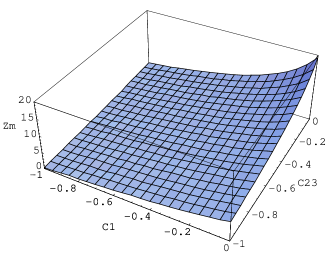
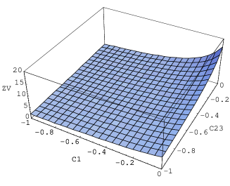
FIG. 2.: Lattice finite part $z_{m}$ for quark mass renormalization factor as a function of $c_{1}$ and $c_{23}$ for clover quark action with $c_{SW}=1$.

FIG. 3.: Lattice finite part $z_{V}$ for vector current as a function of $c_{1}$ and $c_{23}$ for clover quark action with $c_{SW}=1$.

FIG. 4.: Lattice finite part $z_{A}$ for axial vector current as a function of $c_{1}$ and $c_{23}$ for clover quark action with $c_{SW}=1$.

REFERENCES

[1] A. Gonzales-Arroyo, F. J. Yndurain and G. Martinelli,
Phys. Lett. 117B (1982) 437.
[2] G. Martinelli and Y. Zhang,
Phys. Lett. 123B (1983) 433.
[3]R. Groot, J. Hoek and J. Smit,
Nucl. Phys. B237 (1984) 111.
[4] G. Martinelli,
Phys. Lett. 141B (1984) 395.
[5]C. Bernard, A. Soni and T. Draper,
Phys. ReV. D36 (1987) 3224.
[6]G. Curci, E. Franco, L. Miani and G. Martinelli,
Phys. Lett. B202 (1988) 363.
[7]H. Hamber and C. M. Wu,
Phys. Lett. 133B (1983) 351.
[8]E. Gabrielli, G. Martinelli, C. Pittori, G. Heatlie,
and C. T. Sachrajda,
Nucl. Phys. B362 (1991) 475.
[9]R. Frezzotti, E. Gabrielli, C. Pittori and G. C. Rossi,
Nucl. Phys. B373 (1992) 781.
[10]A. Borrelli, C. Pittori, R. Frezzotti and E. Gabrielli,
Nucl. Phys. B409 (1993) 382.
[11] M. Lüscher and P. Weisz,
Nucl. Phys. B479 (1996) 429.
[12] S. Sint and P. Weisz, hep-lat/9704001.
[13]B. Sheikholeslami and R. Wohlert,
Nucl. Phys. B259 (1985) 572.
[14] G. Heatlie, C. T. Sachrajda, G. Martinelli, C. Pittori
and G. C. Rossi,
Nucl. Phys. B352 (1991) 266
[15]CP-PACS Collaboration, S. Aoki, G. Boyd, R. Burkhalter,
S. Hashimoto, N. Ishizuka, Y. Iwasaki, K. Kanaya, T. Kaneko,
Y. Kuramashi, M. Okawa, A. Ukawa and T. Yoshi,̈
Nucl. Phys. B(Proc. Suppl.)60A (1998) 335;
hep-lat/9710059.
[17]P. Weisz,
Nucl. Phys. B212 (1983) 1;
P. Weisz and R. Wohlert,
Nucl. Phys. B236 (1984) 397 ; erratum, ibid. B247 (1984) 544
[18]M. Lüscher and P. Weisz,
Commun. Mth. Phys. 97 (1985) 59.
[19]K. G. Wilson, in Recent Development of Gauge
Theories, eds. G. ’tHooft et al. (Plenum, New York, 1980).
[20] S. Sint, unpublished report.
[21] A. Hasenfratz and P. Hasenfratz,
Phys. Lett. 93B (1980) 165; Nucl. Phys. B193 (1981) 210.
[22] R. Dashen and D. Gross,
Phys. Rev. D23 (1981) 2340.
[23] H. Kawai, R. Nakayama and K. Seo,
Nucl. Phys. B189 (1981) 40.
[24] P. H. Weisz,
Phys. Lett. 100B (1981) 331.
[25] A. Ukawa and S.-K. Yang,
Phys. Lett. 137B (1984) 201
[26] Y. Iwasaki and S. Sakai,
Nucl. Phys. B248 (1984) 441;
Y. Iwasaki and T. Yoshie,
Phys. Lett. 143B (1984) 449.
[27]S. Sint and R. Sommer,
Nucl. Phys. B465 (1996) 71.
[28]A. X. El-Khadra, G. M. Hockney, A. S. Kronfeld and
P. B. Mackenzie,
Phys. Rev. Lett. 69 (1992) 729.