Probing the QCD Vacuum with Static Sources
in Maximal Abelian Projection

1 Introduction

The mechanism of colour confinement is deeply connected with the structure of the QCD vacuum. In the scenario of ’t Hooft and Mandelstam, confinement is viewed as the strong interaction analogue of the well known Meißner effect, in a dual superconductor[1, 2].

As we heard in the introductory lectures by Prof. DiGiacomo during this workshop, the underlying idea is that the QCD vacuum is filled by a chromo-magnetic monopole condensate. Thus, if we insert static colour charges in form of a heavy quark-antiquark pair, $Q\overline{Q}$, the monopole condensate will expel the chromo-electric field from the vacuum. This would then provide the mechanism for chromo-electric flux tube formation and the ensuing linearly rising potential.

On the level of the potential this picture has been verified with progressively refined techniques of lattice gauge theory, ever since the seminal paper of Creutz[3], both in pure gauge theory[4] and full QCD[5].

We would expect that a detailed determination of the flux tube profile between static quarks offers additional insight into the understanding of quark confinement. According to the above scenario, we should observe a normal conducting vortex string that distorts the surrounding superconducting vacuum inside a penetration region of size characterised by the inverse “dual photon” mass, $\lambda$. It is this very transition region between the normal conducting vortex and the undistorted vacuum which is supposed to reveal the interesting physics.

In particular one would hope to gain, from a study of such surface phenomena at the boundary of a dual superconductor, another insight on the second physical scale of spontaneous symmetry breaking, namely the coherence length $\xi$ which is related to the Abelian Higgs mass behind the monopole condensate. This prospect would be highly welcome, as it appears not at all straightforward to attain the Higgs mass directly from correlators between monopole creation/annihilation operators in the purely gluonic sector. Needless to say, though, that the viability of the response-to-source-insertion approach needs to be demonstrated.

It is to be noted that a numerical investigation of the ’t Hooft-Mandelstam scenario requires recourse to an Abelian gauge, such as the maximal Abelian gauge projection (MAGP) proposed in Ref.[7], in order to make contact to Abelian monopoles. In an impressive series of studies the Kanazawa group has established that MAGP indeed accounts for most of the string tension[8]. Moreover, it was shown recently that uncertainties on this result, due to gauge ambiguities in the actual projection procedure on the lattice, can be largely excluded; in fact it was shown that the Abelian part of the string tension accounts for 92 % of the confinement part in the static lattice potential[9].

Another important observation is that expectation values of field distributions suffer much less from stochastic fluctuations after MAGP[10]. As we can demonstrate in Fig. 1, this feature enables us to study string formation over separations as large as $2$ fm in SU(2) gauge theory. This is to be compared to standard SU(2) analyses, where so far energy density distributions of the flux tube disappeared in the noise at string elongations beyond $0.7$ fm[6].

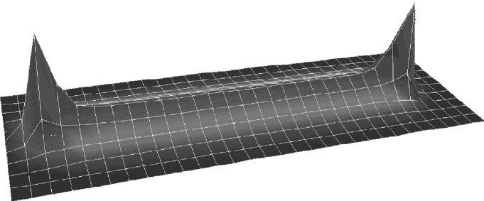
Fig. 1: Energy distribution within a flux tube of length $2$ fm between a $Q\overline{Q}$ pair in MAGP.

First attempts to determine the transverse flux tube profiles in MAGP were launched some years ago in a number of pioneering papers by Haymaker[11] et al. as well as by the Bari[12] and Kanazawa[13] groups. However, these authors had to work with relatively small lattices and $Q\overline{Q}$ separations where the flux tube has not yet fully developed, or non-optimised noise-reduction techniques; as a result previous estimates for the penetration length $\lambda$ and the Ginzburg-Landau coherence length $\xi$[14] suffered from uncontrolled systematic errors and were by far not conclusive.

In the work reported here which is based on the thesis of one of us (Ch.S.), we will try to go much beyond these early attempts, by performing a simulation on a $32^{4}$ lattice at $\beta=2.5115$ (with the SU(2) Wilson action). The salient features of our analysis are: (a) we are well positioned in the scaling regime; (b) we operate at fairly fine lattice spacing, $a=0.086$ fm as to resolve the penetration region (estimated from the string tension $\sqrt{\kappa}=440$ MeV); (c) we are working on a lattice large enough to attain $1$ fm separations between the sources.

We thus expect to meet a fair chance for establishing an observational window towards the boundary phenomena in quest, being safely located between the Scylla and Charybdis regimes of lattice artefacts and poor signal-to-noise ratios.

2 Measuring the Flux Tube

Our present work is based on 116 independent SU(2) gauge configurations that are gauge fixed and projected onto maximal Abelian gauge according to the procedures described in Ref.[9].

After MAGP, the static $Q\overline{Q}$ sources are implemented by considering smeared $R\times T$ Wilson loops, $W(R,T)$, placed between time slices $0$ and $T$ on the lattice. The field distributions around these static objects are determined by measuring correlations with suitable operators, say probes $O({\mathbf{x}},T/2)$. Thus, by varying $\mathbf{x}$ we can survey the environment of two static sources separated by a physical distance $Ra$ from each other. Depending on the choice of the local probe $O$ we can measure the distributions of ${\mathbf{E}}$, ${\mathbf{B}}$, magnetic current ${\mathbf{k}}$ and their curls, divergences etc.

The physics information is retrieved from correlators of type,

$$\langle O({\mathbf{x}},T)\rangle=\frac{\langle O({\mathbf{x}},T/2)W(R,T)\rangle}{\langle W(R,T)\rangle}-\langle O\rangle,$$ (2.1)

in the limit of large $T$. Note that we use smeared Wilson loops in order to achieve good signals (plateaus) at small values of $T$[6, 16].

2.1 Prerequisites: Checking Dual London Equations

At the outset we might wonder whether we are sensitive enough to spot the origin of the chromo-electric fields to the locations of the $Q\overline{Q}$ pair. In fact we find $\mbox{div}\,{\mathbf{E}}$ to vanish nicely outside these sources, as illustrated in Fig. 2.

Fig. 2: Checking the localisations of $\mbox{div}\,\mathbf{E}$ on source and sink, at $R=15$.

An important ingredient of the dual theory is given by the magnetic monopole current, $\mathbf{k}$, which we assume to be defined on our lattice by the standard DeGrand-Toussaint prescription[17]. The expectation is, of course, that this current is a solenoidal (i.e. azimuthal) supercurrent, stabilising the normal conducting vortex core, and fulfilling the dual Ampère Law,

$${\mathbf{k}}=\mbox{curl}\,{\mathbf{E}}$$ (2.2)

Indeed we find $\mathbf{E}$ to be longitudinal and both, $\mbox{curl}\,{\mathbf{E}}$ and ${\mathbf{k}}$, to be purely azimuthal in the centre-plane between the sources. Moreover the equality, Eq. (2.2) is strikingly well obeyed by our data, as visualised in Fig. 3, which exemplifies the situation for $R=8$. This finding provides both support for the superconductivity scenario and an a posteriori justification of the underlying construction of the Abelian monopole current!

Fig. 3: Checking the dual Ampère Law, Eq. (2.2).

In the dual situation, the Cooper pairs from standard superconductivity are replaced by a condensate of magnetic monopoles, and their linear extension is now transcribed into a correlation length, $\xi$. The latter can be retrieved either from the monopole correlator or the coherence length characteristic to the condensate wave function as described by the effective dual Ginzburg-Landau (GL) theory[14]. For small $\xi/\lambda$ ratios, we find ourselves in the deep dual London limit, where $\mathbf{k}$ is directly connected to the chromo-electric vector field, being related to the electric vector potential $\mathbf{A}$ through,

$${\mathbf{E}}=\mbox{curl}\,\mathbf{A}.$$ (2.3)

We consider a colour electric string between charges $Q$ and $\overline{Q}$ placed on the $z$-axis, at $z=0$ and $R$. Let $x$ denote the radial distance of points from the $z$-axis. Combining the London equation in presence of this string,

$$\mbox{curl}\,{\mathbf{k}}=-\frac{1}{\lambda^{2}}\left({\mathbf{E}}-\frac{\mathchar 28936\relax}{2\pi}\delta(x){\mathbf{e}_{z}}\right),$$ (2.4)

with the dual Ampère law, Eq. (2.2), one finds the relation for the $\mathbf{E}$-component, longitudinal to the vortex direction connecting the locations of $Q$ and $\overline{Q}$:

$$E_{z}(x)-\lambda^{2}\mathchar 28929\relax_{2}E_{z}(x)=\frac{\mathchar 28936\relax}{2\pi}\delta^{2}(x),$$ (2.5)

the solution of which is the profile function,

$$E_{z}(x)=\frac{\mathchar 28936\relax}{2\pi\lambda^{2}}K_{0}(x/\lambda).$$ (2.6)

Here $K_{0}$ is the textbook Bessel function, and $\mathchar 28936\relax$ denotes the electric flux associated to the centre vortex.

Fig. 4: Fit of the $E_{z}$-data to the London prediction, Eq. (2.6).

Table I: Fitting $E_{z}$ to Eq. (2.6) at $R=8$, $T=6$ and various fit ranges. $\mu=(\lambda^{2}k)^{-1/2}$ is the dual photon mass, in units of the string tension $k$.

Fit range	$\mathchar 28936\relax$	$\lambda$	$\mu$	$\chi^{2}/{dof}$
1…7.07	1.6(2)	3.6(5)	1.54(21)	1700
2…7.07	1.2(1)	2.4(1)	2.31(10)	150
3…7.07	1.2(1)	2.0(1)	2.77(14)	6
3.1…7.07	1.3(1)	2.0(1)	2.77(14)	9
3.6…7.07	1.4(1)	1.9(1)	2.92(15)	4
4…7.07	1.5(1)	1.88(6)	2.95(09)	1.8
4.2…7.07	1.4(1)	1.82(7)	3.05(12)	1.2
4.5…7.07	1.5(1)	1.82(8)	3.05(13)	1.1
5…7.07	1.5(1)	1.66(7)	3.34(17)	0.7

For the $Q\overline{Q}$ separation $Ra=8a\approx 0.7$ fm, which is well within the flux tube domain, we display the centre-plane distribution of $E_{z}$ in Fig. 4. Our data reveals that these field distributions are well described by the prediction of the dual London theory, Eq. (2.6), iff $x$ is chosen sufficiently deep in vacuo, see Table I. We emphasise that with appropriate lower bounds in the $x$-fit range we gain stable values of $\mathchar 28936\relax$ and $\lambda$. We are therefore in the position to quote rather precise fit values from our dual London limit analysis,

$$\mathchar 28936\relax=1.44(8),\quad\lambda=1.82(7).$$ (2.7)

Note, however, that the value of the chromo-electric flux is far off its (naively) anticipated size which is $\mathchar 28936\relax=1$ for our quarks, carrying one unit of charge! This discrepancy is due to the fact that the parametrisation overestimates the electrical field strength at small $x$.

2.2 Ginzburg-Landau Analysis

The failure of Eq. (2.6) to account for the entire set of $E_{z}$-data hints at the existence of another mass scale, in addition to the dual photon mass, $\lambda^{-1}$. The extraction of this second scale will now be tackled in the framework of the effective dual GL-approach. In our specific axial geometry, the modulus of the wave function, $f$, depends on $x$ alone,

$$\psi=\psi_{\infty}f(x){\rm e}^{i\theta(x)}.$$ (2.8)

Deep inside the vacuum, at $x=\infty$, $f$ is normalised to one. Apart from that, it is controlled by the non-linear GL-equations[15],

$$f(x) = f(x)^{3}+\xi^{2}\left[\left(\frac{1}{x}-\frac{2\pi A_{\theta}(x)}{\mathchar 28936\relax}\right)^{2}-\frac{1}{x}\frac{d}{dx}\left(x\frac{d}{dx}\right)\right]f(x),$$ (2.9)

$$k_{\theta}(x) = \frac{f(x)^{2}}{\lambda^{2}}\left[\frac{\mathchar 28936\relax}{2\pi x}-A_{\theta}(x)\right].$$ (2.10)

Note that previous QCD analyses of these equations were based on modelling the condensate wave function with the ansatz,

$$f(x)=\tanh(x/\alpha)\quad\mbox{with}\quad\quad\alpha=\xi/\nu.$$ (2.11)

In the literature one finds $\nu$ treated as ‘fudge factor’ with ad hoc value chosen to be one. Mind that this arbitrariness in $\nu$ affects the reliability of the value of $\xi$. An examination reveals that the nonlinear character of the GL-equations implies the constraint, from the b.c. at $x=0$:

$$\nu=\sqrt{\frac{3}{8}}\left[1-\frac{3\pi}{4\mathchar 28936\relax}E_{z}(0)\alpha^{2}\right]^{-1/2}.$$ (2.12)

In order to acquire a reliable number for $\nu$, one would evidently need information about $E_{z}(0)$, safe from lattice artefacts — a difficult enterprise.

We will therefore opt for an alternative strategy by utilising the Monte Carlo data (on $\mathbf{E}$ and $\mathbf{k}$) to extract $f$ directly from the GL-equations. To this end we choose parametrisations on $E_{z}$ and $k_{\theta}$ that respect the constraints from the boundary conditions on $f$. In this way we gain access to the physical quantities of interest: $\xi$, $\lambda$, and $\mathchar 28936\relax$, making full use of the structure of the effective dual GL-equations in the continuum.

While for large $x$, $f$ should asymptotically reach the value one, Eq. (2.9) requires $f$ to vanish linearly with $x$ at the centre of the vortex.

Let us remark that at this stage already, $\xi$ is likely to be smaller than $\approx 4$: the reason being that the pure London ansatz proved to be successful in the regime $x\geq 4.2$. Thus our data appear to provide no room for another length scale beyond this point.

To proceed from our data we must first determine $\mathbf{A}$. This is achieved by simple integration over the chromo-electric flux:

$$A_{\theta}(x)=\frac{1}{x}\int_{0}^{x}\!dx^{\prime}x^{\prime}E_{z}(x^{\prime})=\frac{1}{2\pi x}\int\!d^{2}\!f\,E_{z},$$ (2.13)

where $A_{\theta}$ complies with the limiting behaviours,

$$A_{\theta}(x)=\frac{\mathchar 28936\relax}{2\pi x}\quad\quad(x\rightarrow\infty)\quad\mbox{and}\quad A_{\theta}(x)=\frac{E_{z}(0)}{2}x\quad(x\rightarrow 0).$$ (2.14)

Remember that our analysis basically starts out from the second GL-equation, Eq. (2.10) and determines the condensate wave function $f$ from fits to our data for $E_{z}$ (and induced $k_{\theta}$), by use of parametrisations satisfying the boundary conditions on $f$. Eq. (2.10) can be solved for $f/\lambda$,

$$\frac{f(x)}{\lambda}=k^{1/2}_{\theta}(x)\left[\frac{\mathchar 28936\relax}{2\pi x}-A_{\theta}(x)\right]^{-1/2},$$ (2.15)

and cast by use of Eqs. (2.3) and (2.4) into the form

$$f^{2}(x)\int_{x}^{\infty}\!dx^{\prime}x^{\prime}E_{z}(x^{\prime})=-\lambda^{2}x\frac{dE_{z}}{dx}.$$ (2.16)

Fig. 5: Fitting $E_{z}$ with the ansatz, Eq. (2.21), and comparing with data on $E_{z}$ and $k_{\theta}$.

We will now exploit this relation for the determination of $f(x)$. Before we can reach this goal we must find a parametrisation for $E_{z}(x)$ that meets the requirements induced through the boundary conditions on $f$, as set by the GL-equations. Far away from the vortex, where $f\rightarrow 1$, one recovers,

$$E_{z}(x)=-\lambda^{2}\frac{1}{x}\frac{d}{dx}x\frac{dE_{z}}{dx}.$$ (2.17)

From the previous deep London limit solution, $K_{0}(x/\lambda)$, one concludes the asymptotic behaviour $\sim\exp(-x/\lambda)$ for $x\rightarrow\infty$. A good parametrisation for $E_{z}$, which is non singular throughout the entire $x$-interval reads therefore,

$$E_{z}(x)=\frac{\mathchar 28936\relax}{4\pi C_{a}\lambda^{2}}\cosh^{-1}(x/\lambda),$$ (2.18)

where the Catalan constant $C_{a}$ assures the flux to be normalised to $\mathchar 28936\relax$:

$$C_{a}=\sum_{j=0}^{\infty}\frac{\left(-1\right)^{j}}{\left(2j+1\right)^{2}}=0.91596559\ldots.$$ (2.19)

In the vicinity of $x=0$ we expect $f(x)=x/\alpha$. This induces, by Eq. (2.16), the differential equation

$$E_{z}(x)=\alpha^{2}\lambda^{2}\frac{1}{x}\frac{d}{dx}\frac{1}{x}\frac{dE_{z}}{dx},\quad\mbox{with solution}\quad E_{z}(x)=\frac{\mathchar 28936\relax}{\pi\delta^{2}}\exp\left(-\frac{x^{2}}{\delta^{2}}\right),$$ (2.20)

where $\delta=\sqrt{2\alpha\lambda}$. These considerations suggest the following global four-parameter ansatz for our further fitting:

$$E_{z}(x) = \frac{\mathchar 28936\relax}{2\pi}\left[\frac{b}{2C_{a}\lambda^{2}}\frac{1}{\cosh\left(x/\lambda\right)}+\frac{2(1-b)}{\delta^{2}}\exp\left(-\frac{x^{2}}{\delta^{2}}\right)\right],$$ (2.21)

$$k_{\theta}(x) = \frac{\mathchar 28936\relax}{2\pi}\left[\frac{b}{2C_{a}\lambda^{3}}\frac{\tanh(x/\lambda)}{\cosh(x/\lambda)}+\frac{4(1-b)x}{\delta^{4}}\exp\left(-\frac{x^{2}}{\delta^{2}}\right)\right].$$ (2.22)

Fig. 6: $xA_{\theta}$ from numerical integration and from the parametrisation, Eqs. (2.21), (2.23).

Fitting just the data for $E_{z}$ alone results in $\chi^{2}/N_{DF}=21.4/16$, with the parameter values

$$\mathchar 28936\relax=1.08(2),\quad\lambda=1.84(8),\quad\delta=3.28(23),\quad b=0.71(6).$$ (2.23)

Note that the value of $\mathchar 28936\relax$ is now very close to the expectation, yet $\lambda$ being fully consistent with the London limit result, Eq. (2.7). The quality of this fit on $E_{z}$ is exhibited in Fig. 5. However, this very figure also shows that the $k_{\theta}$-data in the region $x\leq 2.2$ are not overly well reproduced with the parameters quoted in Eq. (2.23), despite our convincing confirmation of the dual Ampére Law on the lattice. This, however, is not really unexpected since lattice artefacts are likely to enter the game in this region.

Fig. 7: The boundary region as seen by $E_{z}$ and $f$. $E_{z}$ as in Fig. 5 and $f$ from Eq. (2.15).

To expose the uncertainties from lattice artefacts, we allow next for different values of $\delta$ (say $\delta_{E}$, $\delta_{k}$) in the $E_{z}$ and $k_{\theta}$ parametrisations, Eq. ( 2.21) and obtain a slightly different set of parameter values,

$$\mathchar 28936\relax=1.10(2),\quad\lambda=1.99(5),\quad\delta_{E}=3.03(9),\quad\delta_{k}=3.24(9),\quad b=0.67(3).$$ (2.24)

from a combined fit to the $E_{z}$ and $k_{\theta}$ distributions. The curve in Fig. 3 corresponds to the above parameter values. Although the fit has a reasonable value of $\chi^{2}/N_{DF}=21.4/16$ it is physically not really sensible since it goes along with an unstable, non-monotonic behaviour of $f(x)$, as $\delta_{E}\neq\delta_{k}$. Nevertheless, it provides us with an estimate of discretisation errors.

Before solving Eq. (2.15) for $f$, we numerically integrate $E_{z}$, in order to obtain $xA_{\theta}$. A comparison between numerically integrated data points and integrated parametrisation, Eq. (2.21), is displayed in Fig. 6. The result on $f$ is shown in Fig. 7. The rhs of Eq. (2.15) has been multiplied by $\lambda$ as obtained from a two parameter fit of the data to a $\tanh(x/\alpha)$ ansatz. The parameter values are,

$$\alpha=3.33(5),\quad\lambda=1.62(2),\quad(\chi^{2}/N_{DF}=10.0/17).$$ (2.25)

Fig. 7 visualises the two characteristic scales governing the transverse flux tube profile, one being carried by $E_{z}$, the other being borne by the wave function $f$. Note that the statistical errors on $f$ explode in the region $x>4$, which was indistinguishable from the London limit.

We decide to interprete the differences between the $\lambda$ values above as a systematic uncertainty which we include into the error of our estimate,

$$\lambda=1.84^{+20}_{-24}.$$ (2.26)

Fig. 8: Effective $\xi$ as a function of $x$ with error bands relating to uncertainties in $\alpha$ and $\lambda$.

Let us finally compute $\xi$ from the first GL-equation, Eq. (2.9), by inserting the $\tanh(x/\alpha)$ ansatz for $f(x)$, with $\alpha$ from the fit, Eq. (2.25), and solving Eq. (2.9) locally for $\xi_{\mbox{eff}}(x)$. It is of course not at all guaranteed that the numerical outcome of this procedure is $x$-independent, as it should be: any deviation in $\xi_{\mbox{eff}}(x)$ from a constant reflects systematic uncertainties. In fact we do observe a 30 % variation of $\xi$ as we travel through the transition region, as depicted in Fig. 8. The two error bands correspond to statistical and systematic errors, respectively. This very figure also indicates the window of observation, $2.2<x<4.2$, where we expect to be sensitive to the structure of the wave function. Data obtained at smaller $x$ is unreliable due to lattice artefacts while for large $x$, the uncertainty on $f$ and therefore $\xi$ certainly exceeds the error band suggested by the tanh-parametrisation. Within this window, we find the effective $\xi$ to be

$$\xi=3.10^{+43}_{-35}.$$ (2.27)

This estimate would indicate a GL-parameter $\kappa=\lambda/\xi=0.59^{+13}_{-14}$ which is somewhat below the breakpoint $\kappa=1/\sqrt{2}$ between type II and type I superconductor as indicated in Fig. 8. Our estimate on $\sqrt{2}\lambda$ from Eq. (2.26) is included as the “?” transition region.

3 Discussion

We have verified the validity of the dual Ampère Law in maximal Abelian gauge projection of SU(2) gauge theory. In the London limit analysis of the penetration region around an Abrikosov vortex built up by a static $Q\overline{Q}$ pair, we have found a value of the dual photon mass, $\mu a^{-1}=(\lambda a)^{-1}\approx 3\sqrt{\kappa}$ (Table I), which is well within the ball-park of the known SU(2) glueball masses. In a Ginzburg-Landau analysis, the value of the chromo-electric flux $\mathchar 28936\relax$ is in qualitative agreement with the expected value one while the $\lambda$-value is in accord with the penetration length from the London limit analysis.

We find a small window, $2.2<x<4.2$, within the transition region between vortex and superconducting vacuum from which we can view the GL-wave function and determine the coherence length of the chromo-magnetic condensate. While the wave function varies by about a factor two within this window, the effective value of $\xi$ is constant within 10 %, yielding the value quoted in Eq. (2.27). This appears to be distinctly above the limit $\sqrt{2}\lambda$, indicating that we are faced with a type I superconductor scenario, contrary to previous expectations.

This can only be taken as a tentative conclusion. In order to settle the issue one might study flux profiles with more than one unit of chromo-electric flux involved. It goes without saying that a final answer would require a scaling study as well.

References

- [1] G. ’t Hooft, in High Energy Physics, ed. A. Zichichi (Editorice Compositori Bologna, 1976).
- [2] S. Mandelstam, Phys. Rep. 23C (1976), 245.
- [3] M. Creutz, Phys. Rev. D21 (1974), 2445.
- [4] G.S. Bali and K. Schilling, Phys. Rev. D47 (1993), 661; D46 (1992), 2636; G.S. Bali, K. Schilling, and A. Wachter, Phys. Rev. D56 (1997), 2566.
- [5] SESAM-Collaboration: U. Glässner, S. Güsken, H. Hoeber, Th. Lippert, G. Ritzenhöfer, K. Schilling, G. Siegert, A. Spitz, and A. Wachter, Phys. Lett. B383 (1996), 98.
- [6] G.S. Bali, K. Schilling, and Ch. Schlichter, Phys. Rev. D51 (1995), 5165.
- [7] A.S. Kronfeld, G. Schierholz, and U.-J. Wiese, Nucl. Phys. B293 (1987), 461.
- [8] S. Ejiri, S. Kitahara, T. Suzuki, and K.Yasuta, Phys. Lett. B400 (1997), 163; T. Suzuki, Nucl. Phys. B53 (1997), 531; H. Shiba and T. Suzuki Phys. Lett. B351 (1995), 519.
- [9] G.S. Bali, V. Bornyakov, M. Müller-Preussker, and K. Schilling, Phys. Rev. D54 (1996), 2863.
-
[10]
Ch. Schlichter, Quark Confinement im Szenario
der dualen Supraleitung,
PhD Thesis Wuppertal University, October 1997. - [11] V. Singh, R.W. Haymaker, and D.A. Browne, Phys. Rev. D47 (1993), 1715; Nucl. Phys. B[Proc.Suppl.]30 (1993), 568; Phys. Lett. B306 (1993), 115.
- [12] P. Cea and L. Cosmai, Phys. Rev. D52 (1995), 5152.
- [13] Y. Matsubara, S. Ejiri, and T. Suzuki, Nucl. Phys. B[Proc.Suppl.]34 (1994), 176.
- [14] V.L. Ginzburg and L.D. Landau, Zh. Eksperim. i Teor. Fiz. 20 (1950), 1064.
- [15] see e.g. M. Tinkham, Introduction to Superconductivity, McGraw-Hill, 1975.
- [16] G.S. Bali, Ch. Schlichter and K. Schilling, to be published.
- [17] T.A. DeGrand and D. Toussaint, Phys. Rev. D22 (1980), 2478.