Abstract: Non-perturbative predictions and numerical simulations in supersymmetric Yang-Mills (SYM) theories are reviewed.

1 Introduction

The investigation of non-perturbative properties of supersymmetric (SUSY) gauge theories is presently a rather theoretical subject: it is not known whether (broken) supersymmetry is realized in nature or not. Moreover, the simple (“minimal”) supersymmetric extensions of the standard model do not involve strong interactions near or above the scale of supersymmetry breaking, hence the knowledge of the non-perturbative supersymmetric dynamics is not directly required. In spite of this there is a continuing interest in studying strongly interacting quantum field theories with supersymmetry. (For an early review of the subject see ref. [1].)

The motivation to investigate non-perturbative features of supersymmetric gauge theories is partly coming from the desire to understand relativistic quantum field theories better in general: the supersymmetric points in the parameter space of all quantum field theories are very special since they correspond to situations of a high degree of symmetry. As recent work of Seiberg and Witten [2] and other related papers showed, there is a possibility to approach non-perturbative questions in four dimensional quantum field theories by starting from exact solutions in some highly symmetric points and treat the symmetry breaking as a small perturbation. Beyond this, the knowledge of non-perturbative dynamics in supersymmetric quantum field theories can also be helpful in understanding the greatest puzzle of the standard model, with or without supersymmetric extensions, namely the existence of a large number of seemingly free parameters. As we know from QCD, strong interactions in non-abelian gauge theories are capable to reproduce from a small number of input parameters a large number of dynamically generated parameters for quantities characterizing bound states. This is a possible solution also for the parameters of the standard model if new strong interactions are active beyond the electroweak symmetry breaking scale.

1.1 $N=1$ SYM

The simplest supersymmetric gauge theory is the supersymmetric extension of Yang-Mills theory. The action of Yang-Mills theory with $N=1$ supersymmetry is conventionally given as

$$\int d^{4}x\,d^{2}\theta\,{\rm Tr}(W^{\alpha}W_{\alpha})$$

$$=\int d^{4}x\,{\rm Tr}\left\{-\frac{1}{2}F_{\mu\nu}F^{\mu\nu}+{i\over 2}F_{\mu\nu}\tilde{F}^{\mu\nu}-i\lambda\sigma^{\mu}(D_{\mu}\bar{\lambda})+i(D_{\mu}\bar{\lambda})\bar{\sigma}^{\mu}\lambda+D^{2}\right\}\ ,$$ (1)

where the first line is written in terms of the spinorial field strength superfield $W(x,\theta,\bar{\theta})_{\alpha}$ which depends on the four-coordinate $x$ and the anticommuting Weyl-spinor variables $\theta_{\alpha},\bar{\theta}_{\dot{\alpha}}$ ($\alpha,\dot{\alpha}=1,2$). After performing the Grassmannian integration on $\theta$, one obtains the second form in terms of the component fields. The field strength tensor $F_{\mu\nu}$ and its dual are defined, as usual, as

$$F_{\mu\nu}(x)\equiv-igF_{\mu\nu}^{r}(x)T_{r}\ ,\hskip 30.00005pt\tilde{F}_{\mu\nu}\equiv\frac{1}{2}\epsilon_{\mu\nu\rho\sigma}F^{\rho\sigma}\ .$$ (2)

$\lambda,\bar{\lambda}$ represent a Majorana fermion field in the adjoint representation and $D$ is an auxiliary field.

The action in (1) includes a $\Theta$-term, therefore it is natural to introduce the complex coupling

$$\tau\equiv\frac{\Theta}{2\pi}+\frac{4\pi i}{g^{2}}$$ (3)

and then, with arbitrary $\Theta$, the $N=1$ SYM action becomes:

$$\frac{1}{4\pi}\Im\left\{\tau\int d^{4}x\,d^{2}\theta\,{\rm Tr}(W^{\alpha}W_{\alpha})\right\}$$

$$=\frac{1}{g^{2}}\int d^{4}x\,{\rm Tr}\left[-\frac{1}{2}F_{\mu\nu}F^{\mu\nu}-i\lambda\sigma^{\mu}(D_{\mu}\bar{\lambda})+i(D_{\mu}\bar{\lambda})\bar{\sigma}^{\mu}\lambda+D^{2}\right]$$

$$+\frac{\Theta}{16\pi^{2}}\int d^{4}x\,{\rm Tr}\left[F_{\mu\nu}\tilde{F}^{\mu\nu}\right]\ .$$ (4)

The remarkable feature of the action in (4) is that, after performing the trivial Gaussian integration over the auxiliary field $D$, it is nothing else than an ordinary Yang-Mills action with a massless Majorana fermion in the adjoint representation. This shows that this theory is “automatically” supersymmetric. Introducing a non-zero gaugino mass $m_{\tilde{g}}$ breaks supersymmetry “softly”. Such a mass term is:

$$m_{\tilde{g}}(\lambda^{\alpha}\lambda_{\alpha}+\bar{\lambda}^{\dot{\alpha}}\bar{\lambda}_{\dot{\alpha}})=m_{\tilde{g}}(\bar{\Psi}\Psi)\ .$$ (5)

Here in the first form the Majorana-Weyl components $\lambda,\bar{\lambda}$ are used, in the second form the Dirac-Majorana field $\Psi$.

The Yang-Mills theory of a Majorana fermion in the adjoint representation is, in a general sense, similar to QCD: besides the special Majorana-feature the only difference is that the fermion is in the adjoint representation and not in the fundamental one. As in QCD, a central feature of low-energy dynamics is the realization of the global chiral symmetry. As there is only a single Majorana adjoint “flavour”, the global chiral symmetry of $N=1$ SYM is $U(1)_{\lambda}$, which coincides with the so called R-symmetry generated by the transformations

$$\theta_{\alpha}^{\prime}=e^{i\varphi}\theta_{\alpha}\ ,\hskip 20.00003pt\bar{\theta}_{\dot{\alpha}}^{\prime}=e^{-i\varphi}\bar{\theta}_{\dot{\alpha}}\ .$$ (6)

This is equivalent to

$$\lambda_{\alpha}^{\prime}=e^{i\varphi}\lambda_{\alpha}\ ,\hskip 5.0pt\bar{\lambda}_{\dot{\alpha}}^{\prime}=e^{-i\varphi}\bar{\lambda}_{\dot{\alpha}}\ ,\hskip 5.0pt\Psi^{\prime}=e^{-i\varphi\gamma_{5}}\Psi\ .$$ (7)

The $U(1)_{\lambda}$-symmetry is anomalous: for the corresponding axial current $J_{\mu}\equiv\bar{\Psi}\gamma_{\mu}\gamma_{5}\Psi$, in case of $SU(N_{c})$ gauge group with coupling $g$, we have

$$\partial^{\mu}J_{\mu}=\frac{N_{c}g^{2}}{32\pi^{2}}\epsilon^{\mu\nu\rho\sigma}F_{\mu\nu}^{r}F_{\rho\sigma}^{r}\ .$$ (8)

However, the anomaly leaves a $Z_{2N_{c}}$ subgroup of $U(1)_{\lambda}$ unbroken. This can be seen, for instance, by noting that the transformations

$$\Psi\to e^{-i\varphi\gamma_{5}}\Psi\ ,\hskip 20.00003pt\bar{\Psi}\to\bar{\Psi}e^{-i\varphi\gamma_{5}}$$ (9)

are equivalent to

$$m_{\tilde{g}}\to m_{\tilde{g}}e^{-2i\varphi\gamma_{5}}\ ,\;\Theta_{SYM}\to\Theta_{SYM}-2N_{c}\varphi\ ,$$ (10)

where $\Theta_{SYM}$ is the $\Theta$-parameter of gauge dynamics. Since $\Theta_{SYM}$ is periodic with period $2\pi$, for $m_{\tilde{g}}=0$ the $U(1)_{\lambda}$ symmetry is unbroken if

$$\varphi=\varphi_{k}\equiv\frac{k\pi}{N_{c}}\ ,\hskip 20.00003pt(k=0,1,\ldots,2N_{c}-1)\ .$$ (11)

For this statement it is essential that the topological charge is integer.

The discrete global chiral symmetry $Z_{2N_{c}}$ is expected to be spontaneously broken by the non-zero gaugino condensate $\langle\lambda\lambda\rangle\neq 0$ to $Z_{2}$ defined by $\{\varphi_{0},\varphi_{N_{c}}\}$ (note that $\lambda\to-\lambda$ is a rotation). The consequence of this spontaneous chiral symmetry breaking pattern is the existence of a first order phase transition at zero gaugino mass $m_{\tilde{g}}=0$. For instance, in case of $N_{c}=2$ there exist two degenerate ground states with opposite signs of the gaugino condensate. The symmetry breaking is linear in $m_{\tilde{g}}$, therefore the two ground states are exchanged at $m_{\tilde{g}}=0$ and there is a first order phase transition.

The non-perturbative features of the SYM theory can be investigated in a lattice formulation. As always, the lattice action is not unique (see section 3.1). A possible formulation was given by Curci and Veneziano [3] based on the well known lattice formulation of QCD introduced by Wilson. In the lattice action the bare gauge coupling (of $SU(N_{c})$) is convetionally represented by $\beta\equiv 2N_{c}/g^{2}$ and the bare gaugino mass by the hopping parameter $K$. In the plane of ($\beta,K$) there is a critical line corresponding to zero gaugino mass and the expected phase structure is the one shown in figure 1.

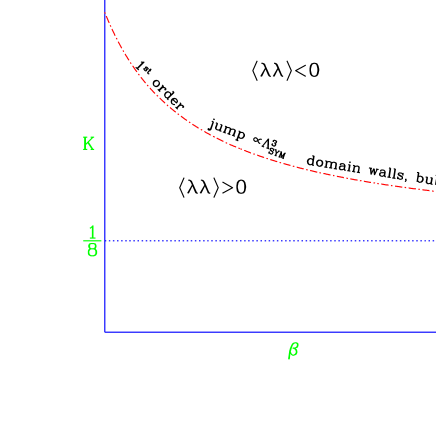
Figure 1: Expected phase structure of SU(2) Yang-Mills theory with a Majorana fermion in adjoint representation in the ($\beta,K$)-plane. The dashed-dotted line is a first order phase transition at zero gluino mass, where supersymmetry is expected.

1.2 $N=2$ SYM

The SYM theory with $N=2$ extended supersymmetry is a highly constrained theory which has, however, more structure than the relatively simple $N=1$ case discussed above. In particular, besides the $N=1$ “vector superfield” containing the gauge boson and gaugino $(A_{\mu},\lambda)$, it also involves an $N=1$ “chiral superfield” $(\phi,\lambda^{\prime})$ in the adjoint representation which consists of the complex scalar $\phi\equiv A+iB$ and the Majorana fermion $\lambda^{\prime}$. The Majorana pair $(\lambda,\lambda^{\prime})$ can be combined to a Dirac-fermion $\psi$ and then the vector-like (non-chiral) nature of this theory can be made explicit.

The Euclidean action of $N=2$ SYM theory in component notation, for simplicity in case of an SU(2) gauge group, is the following:

$$S_{SYM}^{N=2}=\int d^{4}x\;\raisebox{-1.29167pt}{\mbox{\LARGE$\left\{\right.$}}{1\over 4}F_{\mu\nu}^{r}(x)F_{\mu\nu}^{r}(x)+\frac{1}{2}(D_{\mu}A^{r}(x))(D_{\mu}A^{r}(x))+\frac{1}{2}(D_{\mu}B^{r}(x))(D_{\mu}B^{r}(x))$$

$$+\overline{\psi}^{r}(x)\gamma_{\mu}D_{\mu}\psi^{r}(x)+ig\epsilon_{rst}\overline{\psi}^{r}(x)[A^{s}(x)+i\gamma_{5}B^{s}(x)]\psi^{t}(x)$$

$$+\frac{g^{2}}{2}[A^{r}(x)A^{r}(x)B^{s}(x)B^{s}(x)-A^{r}(x)B^{r}(x)A^{s}(x)B^{s}(x)]\raisebox{-1.29167pt}{\mbox{\LARGE$\left.\right\}$}}\ .$$ (12)

This is a massless adjoint Higgs-Yukawa model with special Yukawa- and quartic couplings given in terms of the gauge coupling.

In $N=2$ SUSY possible couplings are so strongly constrained by the symmetry that only gauge couplings are allowed. Another important feature is that the symmetry also implies that the matter field content is always vector-like. Therefore $N=2$ SUSY theories are always non-chiral and hence well suited for lattice sudies. A lattice formulation of $N=2$ SYM based on the Wilsonian formulation of QCD has been investigated in [4].

The main new feature of $N=2$ SYM compared to $N=1$ SYM is that it also contains scalar fields, hence there is the possibility of Higgs mechanism. Let us here only consider the simplest case of an $SU(2)$ gauge group. In the Higgs phase the vacuum expectation value of the scalar field is non-zero. In terms of the real components $\phi(x)\equiv A(x)+iB(x)$ we have

$$\langle A^{r}(x)\rangle\neq 0\ ,\hskip 20.00003pt\langle B^{r}(x)\rangle\neq 0\ .$$ (13)

This implies the Higgs mechanism breaking of $SU(2)\to U(1)$, similarly to the Georgi-Glashow model. Due to the Higgs mechanism the “charged” gauge bosons become heavy. The low-energy effective theory is $N=2$ SYM with $U(1)$ gauge group.

Seiber and Witten proved [2] that extended SUSY and asymptotic freedom can be exploited to determine exactly the low-energy effective action in the Higgs phase, if the vacuum expectation values are large. At strong couplings there are two singularities of the effective action corresponding to light monopoles and dyons, respectively.

The expectation value of the complex scalar field $\langle\phi\rangle$ parametrizes the moduli space of zero-energy degenerate vacua. The degeneracy is a consequence of $N=2$ supersymmetry. This phenomenon is usually referred to as the existence of flat directions: the potential identically vanishes for $B^{r}=cA^{r}$. In the present case the moduli space is a non-compact manifold with two parameters. The presence of non-compact flat directions requires the breaking of supersymmetry for the definition of the path integral over the scalar fields: otherwise the path integral would be divergent. It is also plausible that soft breaking with mass terms is not enough in the Higgs phase, where the mass-squared terms in the potential are negative. Therefore small hard breaking by dimensionless couplings is also required.

These arguments are quite general. In the special case of $N=2$ SYM the general renormalizable scalar potential with the given set of scalar fields is

$$V(A,B)\equiv\frac{1}{2}m_{A}^{2}A^{r}A^{r}+\frac{1}{2}m_{B}^{2}B^{r}B^{r}$$

$$+\lambda_{A}(A^{r}A^{r})^{2}+\lambda_{B}(B^{r}B^{r})^{2}+\lambda_{[AB]}A^{r}A^{r}B^{s}B^{s}-\lambda_{(AB)}(A^{r}B^{r})^{2}\ .$$ (14)

N=2 supersymmetry is at the point of parameter space where

$$m_{A}=m_{B}=\lambda_{A}=\lambda_{B}=0\ ,\hskip 10.00002pt2\lambda_{[AB]}=2\lambda_{(AB)}=g^{2}\ .$$ (15)

In order that the path integral over the scalar fields be convergent, the quartic couplings have to fulfil the following conditions:

$$\lambda_{A}>0\hskip 20.00003pt{\rm AND}\hskip 20.00003pt\lambda_{B}>0\hskip 20.00003pt{\rm AND}$$

$$\raisebox{-1.29167pt}{\mbox{\LARGE$\left\{\right.$}}\lambda_{[AB]}\geq\max(0,\lambda_{(AB)})\hskip 20.00003pt{\rm OR}\hskip 20.00003pt4\lambda_{A}\lambda_{B}>\max[\lambda_{[AB]}^{2},(\lambda_{[AB]}-\lambda_{(AB)})^{2}]\raisebox{-1.29167pt}{\mbox{\LARGE$\left.\right\}$}}\ .$$ (16)

This is in conflict with the supersymmetry conditions.

The consequence of the conflict between supersymmetry and the convergence of the path integral over the scalar fields is that in a path integral formulation of the quantized theory the supersymmetry has to be broken. On the lattice this means that supersymmetry is broken as long as the lattice spacing is non-zero and can only be restored in the continuum limit $a\to 0$.

The tuning to the supersymmetric point in $N=2$ SYM can be studied, for instance, in lattice perturbation theory [4]. It can be shown that the compact flat direction is reproduced for $a\to 0$ on a specific phase transition where three different kinds of Higgs-phases meet. The emergence of the non-compact flat direction is a result of cancelling of quantum correction contributions from scalars and fermions. This is similar to the situation which occurs if the so called vacuum stability boundary in Higgs-Yukawa models reaches zero fermion mass. (For a lattice investigation of the vacuum stability bound see, for instance, ref. [5].)

2 Non-perturbative predictions for $N=1$ SYM

In analogy with QCD, one expects that the spectrum of the SYM model consists of colourless bound states formed out of the fundamental excitations, namely gluons and gluinos. (In this context we shall use the name “gluino” instead of the more general term “gaugino”.) In the supersymmetric point at zero gluino mass these bound states should be organized in supersymmetry multiplets, according to the representations of the SUSY extension of the Poincaré algebra. For the description of lowest energy bound states one can use an effective field theory in terms of suitably chosen colourless composite operators.

For $N=1$ SYM the effective action was constructed by Veneziano and Yankielowicz (VY) [6]. The composite operator appearing in the VY effective action is a chiral supermultiplet $S$ containing as component fields the expressions for the anomalies [7]:

$$S\equiv A(y)+\sqrt{2}\theta\Psi(y)+\theta^{2}F(y)\ ,$$ (17)

where, for instance, the scalar component is proportional to the gluino bilinear

$$A\propto\lambda^{\alpha}\lambda_{\alpha}\ .$$ (18)

The other components contain gluino-gluino and gluino-gluon combinations. Therefore, as far as a constituent picture is applicable to the bound states formed by strong interactions, the particle content of the lowest supersymmetry multiplet is: a pseudoscalar gluino-gluino bound state, a Majorana spinor gluon-gluino bound state and a scalar gluino-gluino bound state. In terms of $S$ the VY effective action has the form

$$S_{VY}=\frac{1}{\alpha}\int d^{4}x\,d^{2}\theta\,d^{2}\bar{\theta}\,(S^{\dagger}S)^{1/3}+\gamma\,[\int d^{4}x\,d^{2}\theta\,(S\log\frac{S}{\Lambda}-S)+{\rm h.c.}]\ .$$ (19)

Here $\alpha$ and $\gamma$ are positive constants and $\Lambda$ is the usual mass parameter for the asymptotically free coupling defined at scale $\mu$:

$$\Lambda\equiv\mu e^{-{1}/{2\beta_{0}g(\mu)^{2}}}\ ,\hskip 30.00005pt\beta_{0}=\frac{3N_{c}}{16\pi^{2}}\ .$$ (20)

As usual, $\beta_{0}$ denotes the first coefficient of the $\beta$-function and we consider here the gauge group $SU(N_{c})$.

The effective action in (19) incorporates the breaking of the discrete $Z_{2N_{c}}$ chiral symmetry by the gluino condensate

$$\langle\lambda\lambda\rangle=C\Lambda^{3}e^{2\pi ik/N_{c}}\ .$$ (21)

The phase factor depending on the integer $k$ refers to the different ground states defined in (11). The proportionality factor $C$ depends, of course, on the renormalization scheme belonging to $\Lambda$. Instanton calculations and other reasonings imply that we have $C=32\pi^{2}$ in the dimensional reduction scheme $\Lambda=\Lambda_{DR}$ [8].

The main assumption needed to derive the VY effective action (20) is the choice of the chiral superfield $S$ as the dominant degree of freedom of low energy dynamics. Making a more general ansatz also containing gluon-gluon composites leads to a generalization and to two mixed supermultiplets in the low energy spectrum [9]. Even if $S$ is accepted as the dominant variable, one can argue about the existence of a chirally symmetric ground state, in addition to the $N_{c}$ ground states with broken chiral symmetry given by the integer $k<N_{c}$ in (21) [10].

An interesting question is how the spectrum of glueballs, gluinoballs and gluino-glueballs is influenced by the soft supersymmetry breaking due to a non-zero gluino mass $m_{\tilde{g}}\neq 0$. For small $m_{\tilde{g}}$ it is possible to derive the coefficients of the terms linear in $m_{\tilde{g}}$ in the mass formulas [11]. (Note, however, that the two papers in this reference arrive to different results.)

A general consequence of the chiral symmetry breaking is the existence of a first order phase transition at $m_{\tilde{g}}=0$. At this point the different ground states in (21) are degenerate and a coexistence of the corresponding phases is possible. In a mixed phase situation, as usual at first order phase transitions, the different phases are separated by “bubble wall” interfaces. The interface tension of the walls can be exactly derived from the central extension of the $N=1$ SUSY algebra [12]. The result is that the energy density of the interface wall is related to the jump of the gluino condensate by

$$\epsilon=\frac{N_{c}}{8\pi^{2}}\left|\langle\lambda\lambda\rangle_{1}-\langle\lambda\lambda\rangle_{2}\right|\ .$$ (22)

Combining this with eq. (21) implies that the dimensionless ratio $\epsilon/|\langle\lambda\lambda\rangle|$ is predicted independently of the renormalization scheme.

In order to compare the predictions (21) and (22) to the results of lattice Monte Carlo simulations it is convenient to switch to the lattice $\Lambda$-parameter $\Lambda_{LAT}$. First one can use [8]

$$\Lambda_{DR}/\Lambda_{\overline{MS}}=\exp\{-1/18\}$$ (23)

and then for the Curci-Veneziano lattice action [13]

$$\Lambda_{\overline{MS}}/\Lambda_{LAT}=\exp\left\{-\frac{1}{\beta_{0}}\left[\frac{1}{16N_{c}}-N_{c}P+\frac{N_{c}n_{a}}{2}P_{3}\right]\right\}\ ,$$

$$\beta_{0}=\frac{N_{c}}{48\pi^{2}}(11-2n_{a})\ ,\hskip 20.00003ptP=0.0849780(1)\ ,\hskip 20.00003ptP_{3}=0.0066960(1)\ .$$ (24)

Here $n_{a}$ is the number of Majorana fermions in the adjoint representation, that is for SYM we set $n_{a}=1$.

For transforming (21) and (22) to lattice units we need, in fact, the value of $a\Lambda_{LAT}$ at the particular values of interest of the lattice bare parameters $\beta,K$. Before performing the lattice simulations this is, of course, not known. An order of magnitude estimate can be obtained from pure gauge theory (at $K=0$) by noting that both for $N_{c}=2$ and $N_{c}=3$ we have for the lowest gluball mass $M$ [14]

$$a\Lambda_{LAT}\simeq\frac{aM}{200}\ .$$ (25)

Assuming this approximate relation also at the critical line for zero gluino mass, we can use eqs. (21)-(25) for estimating orders of magnitudes. In the region where $aM={\cal O}(1)$ we obtain

$$a^{3}|\langle\lambda\lambda\rangle_{1}-\langle\lambda\lambda\rangle_{2}|={\cal O}(1)\ ,\hskip 30.00005pta^{3}\epsilon={\cal O}(10^{-1})\ .$$ (26)

As these numbers show, the predicted first order phase transition is, in fact, strong enough for a relatively easy observation in lattice simulations.

3 Numerical Monte Carlo simulations

The lattice Monte Carlo simulations of quantum field theories are performed in Euclidean space-time. For SYM, and more generally for a Yang-Mills theory of Majorana fermions in the adjoint representation (“gaugino” or in the context of strong interactions “gluino”) with arbitrary mass we need first of all the definition of Majorana fermions in Euclidean space-time.

In the literature one may sometimes find the statement that there are no Euclidean Majorana spinors (see, for instance, [15]). This is only true as long as one is concentrating on the hermiticity properties of fields, as in Minkowski space. The definition required for an Euclidean path integral can be based on the appropriate analytic continuation of expectation values [16]. The essential point is that for Majorana fermions the Grassmann variables $\Psi$ and $\overline{\Psi}$ are not independent, as is the case for Dirac fermions, but are related by

$$\overline{\Psi}=\Psi^{T}C\ ,$$ (27)

with $C$ the charge conjugation Dirac matrix. In fact, starting from an Euclidean Dirac fermion field represented by the pair $\psi,\overline{\psi}$ one can define two Majorana fermion fields satisfying (27) by

$$\Psi^{(1)}\equiv\frac{1}{\sqrt{2}}(\psi+C\overline{\psi}^{T})\ ,\hskip 20.00003pt\Psi^{(2)}\equiv\frac{i}{\sqrt{2}}(-\psi+C\overline{\psi}^{T})\ .$$ (28)

Using also the inverse relations

$$\psi=\frac{1}{\sqrt{2}}(\Psi^{(1)}+i\Psi^{(2)})\ ,\hskip 20.00003pt\psi_{c}\equiv C\overline{\psi}^{T}=\frac{1}{\sqrt{2}}(\Psi^{(1)}-i\Psi^{(2)})\ ,$$ (29)

one can easily relate expectation values of Majorana and Dirac fermion fields [17].

3.1 Lattice actions and algorithms

Following Curci and Veneziano [3], we can take for the fermionic part of the SYM action the well known Wilson formulation. If the Grassmanian fermion fields in the adjoint representation are denoted by $\psi^{r}_{x}$ and $\overline{\psi}^{r}_{x}$, with $r$ being the adjoint representation index ($r=1,..,N_{c}^{2}-1$ for SU($N_{c}$) ), then the fermionic part of the lattice action is:

$$S_{f}=\sum_{x}\raisebox{-1.29167pt}{\mbox{\LARGE$\left\{\right.$}}\overline{\psi}_{x}^{r}\psi_{x}^{r}-K\sum_{\mu=1}^{4}\left[\overline{\psi}_{x+\hat{\mu}}^{r}V_{rs,x\mu}(1+\gamma_{\mu})\psi_{x}^{s}+\overline{\psi}_{x}^{r}V_{rs,x\mu}^{T}(1-\gamma_{\mu})\psi_{x+\hat{\mu}}^{s}\right]\raisebox{-1.29167pt}{\mbox{\LARGE$\left.\right\}$}}\ .$$ (30)

Here $K$ is the hopping parameter, the irrelevant Wilson parameter removing the fermion doublers in the continuum limit is fixed to $r=1$, and the matrix for the gauge-field link in the adjoint representation is defined as

$$V_{rs,x\mu}\equiv V_{rs,x\mu}[U]\equiv 2{\rm Tr}(U_{x\mu}^{\dagger}T_{r}U_{x\mu}T_{s})=V_{rs,x\mu}^{*}=V_{rs,x\mu}^{-1T}\ .$$ (31)

The generators $T_{r}\equiv\frac{1}{2}\lambda_{r}$ satisfy the usual normalization ${\rm Tr\,}(\lambda_{r}\lambda_{s})=\frac{1}{2}$. In case of SU(2) ($N_{c}=2$) we have $T_{r}\equiv\frac{1}{2}\tau_{r}$ with the isospin Pauli-matrices $\tau_{r}$. The normalization of the fermion fields in (30) is the usual one for numerical simulations. The full lattice action is the sum of the pure gauge part and fermionic part:

$$S=S_{g}+S_{f}\ .$$ (32)

Here the standard Wilson action for the SU($N_{c}$) gauge field $S_{g}$ is a sum over the plaquettes

$$S_{g}=\beta\sum_{pl}\left(1-\frac{1}{N_{c}}{\rm Re\,Tr\,}U_{pl}\right)\ ,$$ (33)

with the bare gauge coupling given by $\beta\equiv 2N_{c}/g^{2}$.

Using the relations in (29) one can decompose $S_{f}$ as a sum over the two Majorana components:

$$S_{f}=\sum_{xu,yv}\overline{\psi}^{v}_{y}Q_{yv,xu}\psi^{u}_{x}=\frac{1}{2}\sum_{j=1}^{2}\sum_{xu,yv}\overline{\Psi}^{(j)v}_{y}Q_{yv,xu}\Psi^{(j)u}_{x}\ ,$$ (34)

where the fermion matrix $Q$ is defined in (30). Using this, the fermionic path integral for Dirac fermions can be written as

$$\int[d\overline{\psi}d\psi]e^{-S_{f}}=\int[d\overline{\psi}d\psi]e^{-\overline{\psi}Q\psi}=\det Q=\prod_{j=1}^{2}\int[d\Psi^{(j)}]e^{-\frac{1}{2}\overline{\Psi}^{(j)}Q\Psi^{(j)}}\ .$$ (35)

For Majorana fields the path integral involves only $[d\Psi^{(j)}]$, either with $j=1$ or $j=2$. For $\Psi\equiv\Psi^{(1)}$ or $\Psi\equiv\Psi^{(2)}$ we have

$$\int[d\Psi]e^{-\frac{1}{2}\overline{\Psi}Q\Psi}=\pm\sqrt{\det Q}\ .$$ (36)

In order to define the sign in (36) one has to consider the Pfaffian of the antisymmetric matrix

$$M\equiv CQ\ .$$ (37)

This can be defined for a general complex antisymmetric matrix $M_{\alpha\beta}=-M_{\beta\alpha}$ with an even number of dimensions ($1\leq\alpha,\beta\leq 2N$) by a Grassmann integral as

$${\rm Pf}(M)\equiv\int[d\phi]e^{-\frac{1}{2}\phi_{\alpha}M_{\alpha\beta}\phi_{\beta}}=\frac{1}{N!2^{N}}\epsilon_{\alpha_{1}\beta_{1}\ldots\alpha_{N}\beta_{N}}M_{\alpha_{1}\beta_{1}}\ldots M_{\alpha_{N}\beta_{N}}\ .$$ (38)

Here, of course, $[d\phi]\equiv d\phi_{2N}\ldots d\phi_{1}$, and $\epsilon$ is the totally antisymmetric unit tensor. One can easily show that

$$\left[{\rm Pf}(M)\right]^{2}=\det M\ .$$ (39)

If $M$ is taken from (37) one also has $\det M=\det Q$.

The relations in (36) or (39) show that, in order to represent a Majorana fermion, in the path integral over the gauge field the square root of the fermion determinant (or the Pfaffian of the matrix in (37)) has to be taken. In this sense a Majorana fermion corresponds to a flavour number $\frac{1}{2}$. Concerning the sign of the square root, in numerical simulations it is easier to take always the absolute value. This presumably does not have an influence in the continuum limit because in the continuum the (real) eigenvalues of the Dirac matrix come in pairs and the square root is always positive (see, for instance, [18]).

In general, the lattice action describing a given “target” continuum quantum field theory is not unique. Besides the Curci-Veneziano action discussed up to now, another possibility is based on five-dimensional domain walls [19, 20, 21]. In this approach one knows the value of the bare fermion mass where the supersymmetric continuum limit is best approached and one has advantages from the point of view of the speed of symmetry restoration. The price one has to pay is the proliferation of (auxiliary) fermion flavours. Another proposal for reaching supersymmetric quantum field theories is to try direct dimensional reduction on the lattice [22].

In order to perform Monte Carlo simulations with effective flavour number $\frac{1}{2}$ corresponding to Majorana fermions in the lattice formulation of Curci and Veneziano, one can either use the multi-bosonic technique [23, 17] or apply the hybrid classical dynamics algorithm [24]. Exploratory studies have been started recently. (For a recent review and status report see [25].)

The first step in numerical simulations is to consider the quenched approximation, which neglects the dynamical effects of gluinos [26, 27]. Since quenching breaks supersymmetry explicitly, this mainly serves as a testing ground for mass measurements and helps to localize the physically interesting bare parameter range.

A first large scale numerical simulation of SU(2) SYM with dynamical gluinos has been started recently by the DESY-Münster collaboration [28] using the supercomputers at HLRZ, Jülich and DESY, Zeuthen. The main goals of this collaboration are: to find the first order phase transition at zero gluino mass and to determine the masses of the lowest bound states formed out of gluons and gluinos in the interesting range of the gluino mass.

Acknowledgements

I thank Peter Weisz for correspondence and for communicating his result on the ratio of $\Lambda$-parameters in (24).

References

- [1] D. Amati, K. Konishi, Y. Meurice, G.C. Rossi and G. Veneziano, Phys. Rep. 162 (1988) 169
- [2] N. Seiberg and E. Witten, Nucl. Phys. B426 (1994) 19; ERRATUM ibid. B430 (1994) 485
- [3] G. Curci and G. Veneziano, Nucl. Phys. B292 (1987) 555
- [4] I. Montvay, Phys. Lett. B344 (1995) 176 and Nucl. Phys. B445 (1995) 399
- [5] L. Lin, I. Montvay, G. Münster, M. Plagge, H. Wittig, Phys. Lett. B317 (1993) 143
- [6] G. Veneziano, S. Yankielowicz, Phys. Lett. B113 (1982) 231
- [7] S. Ferrara, B. Zumino, Nucl. Phys. B87 (1975) 207
- [8] D. Finnell, P. Pouliot, Nucl. Phys. B453 (1995) 225.
- [9] G.R. Farrar, G. Gabadadze, M. Schwetz, hep-th/9711166
- [10] A. Kovner, M. Shifman, Phys. Rev. D56 (1997) 2396
-
[11]
A. Masiero, G. Veneziano,
Nucl. Phys. B249 (1985) 593;
N. Evans, S.D.H. Hsu, M. Schwetz, hep-th/9707260. - [12] A. Kovner, M. Shifman, A. Smilga, Phys. Rev. D56 (1997) 7978
-
[13]
A. Hasenfratz, P. Hasenfratz,
Phys. Lett. 93B (1980) 165;
P. Weisz, Phys. Lett. 100B (1981) 331 and private communication -
[14]
C. Michael, M. Teper,
Phys. Lett. B199 (1987) 95;
H. Chen, J. Sexton, A. Vaccarino, D. Weingarten, Nucl. Phys. Proc. Suppl. 34 (1994) 357;
M.J. Teper, hep-lat/9711011 - [15] H. Leutwyler, A. Smilga, Phys. Rev. D46 (1992) 5607
-
[16]
H. Nicolai,
Nucl. Phys. B140 (1978) 294;
P. van Nieuwenhuizen, A. Waldron, Phys. Lett. B389 (1996) 29 - [17] I. Montvay, Nucl. Phys. B466 (1996) 259
- [18] S.D.H. Hsu, hep-th/9704149
-
[19]
R. Narayanan, H. Neuberger,
Nucl. Phys. B443 (1995) 305;
P. Huet, R. Narayanan, H. Neuberger, Phys. Lett. B380 (1996) 291;
H. Neuberger, hep-lat/9710089 -
[20]
J. Nishimura,
Phys. Lett. B406 (1997) 215 and hep-lat/9709112;
T. Hotta, T. Izubuchi, J. Nishimura, hep-lat/9709075 and hep-lat/9712009 - [21] S. Aoki, K. Nagai, S.V. Zenkin, Nucl. Phys. B508 (1997) 715 and hep-lat/9709058.
- [22] N. Maru, J. Nishimura, hep-th/9705152
- [23] M. Lüscher, Nucl. Phys. B418 (1994) 637
- [24] A. Donini, M. Guagnelli, Phys. Lett. B383 (1996) 301
- [25] I. Montvay, hep-lat/9709080, to appear in the Proceedings of the Lattice ’97 Conference in Edinburgh.
- [26] G. Koutsoumbas, I. Montvay, Phys. Lett. B398 (1997) 130
- [27] A. Donini, M. Guagnelli, P. Hernandez, A. Vladikas, hep-lat/9708006 and hep-lat/9710065.
- [28] G. Koutsoumbas, I. Montvay, A. Pap, K. Spanderen, D. Talkenberger, J. Westphalen, hep-lat/9709091, to appear in the Proceedings of the Lattice ’97 Conference in Edinburgh.