Topology, fermionic zero modes and flavor singlet correlators in finite temperature QCD.

Abstract

We compute the screening correlators in the $\sigma$ and $\eta^{\prime}$ flavor singlet channels in finite temperature QCD with 2 light quark flavors. Together with the correlators in the $\vec{\pi}$ and $\vec{\delta}$ channels, these are used to discuss several issues related to symmetry restoration and the nature of the QCD phase transition. Our calculations span a range of temperature extending from approximately 125 MeV to 170 MeV and are carried out in the context of a staggered fermion formulation on a $16^{3}\times 8$ lattice. In addition to the computation at a fixed quark mass ($am_{q}=0.00625$), we discuss the issue of the chiral limit. After careful consideration of the zero-mode shift lattice artefact, we present rather strong (topological) arguments in favor of the non-restoration of $U_{A}(1)$ at $T_{c}$.

I INTRODUCTION

The lattice approach has been quite successful in describing the general aspects of the finite temperature QCD phase transition (for recent reviews see [1, 2, 3]). However the advent of relativistic heavy ion experiments as well as purely theoretical motivations calls for even more precise and quantitative simulations. Questions such as the determination of the critical exponents and the universality class of the phase transition (assuming a second order transition, which is favored but not yet proven [1]) still have to be answered in detail. Among other things, this will require simulations at [4] or close to the chiral limit and may necessitate new simulation algorithms. In this paper, we would like to delineate a small subset of the issues that one is likely to encounter as part of such a program: namely, those questions which are associated with the anomalous U(1) axial symmetry. This includes a measurement of flavor singlet mesonic correlators together with the extraction of flavor singlet susceptibilities and screening lengths (section IV) and lays the groundwork for a study of the interplay between topology and the chiral phase transition (section V). These topics are closely related to a question which has recently attracted much attention in the literature [5, 6], namely “which chiral symmetry is restored at the finite temperature phase transition ?”. Attempts at general proofs in the continuum that $U_{A}(1)$ should be restored at $T_{c}$ [7] have been shown to be flawed [8, 9] . In fact, lattice simulations seem to indicate that this symmetry is only restored at higher temperatures [10, 11] (although there remain real uncertainties concerning the proper method of extrapolation to the chiral limit [11, 12]). In this paper, we identify the zero-mode shift phenomenon [13] as a clear source of difficulties in the chiral limit (see section VI). We therefore take the position that a rigorous quantitative extrapolation to the chiral limit will only be possible once this problem has been solved. For the time being, we do two things: first, we work at a fixed but small value of the quark mass ($ma=0.00625$ in lattice units) and vary the temperature (thereby exploring the direction orthogonal to refs. [11, 12]). Then we use general topological arguments (i.e. the Atiyah-Singer index theorem) to decide on the question of restoration or non-restoration of the $U_{A}(1)$ symmetry. We also realize that at present, the investigation of topics related to topology is only possible in finite volumes and leave the questions related to the extrapolation to the infinite volume limit for future studies.

The measurement of flavor singlet meson correlators and screening lengths at finite temperature (section IV) had not been attempted previously , but is quite important both theoretically and phenomenologically. First, the $\sigma$ (flavor singlet scalar meson) is the degree of freedom which becomes light at the transition (again assuming a second order phase transition) and therefore drives the long distance dynamics together with the pion. Second, a determination of the temperature at which the $U(1)$ axial symmetry is effectively restored is very interesting because it will affect the production rate of $\eta^{\prime}$ mesons (relative to pions for example) in relativistic heavy ion collisions [15, 16]. Some of the questions considered here have also been investigated through different methods: instanton simulations were used in [17] and Nambu Jona-Lasinio models in [18].

In view of the existence of the lattice artefacts mentioned above, we adopt in this paper a two step strategy to study the restoration of symmetries in finite temperature QCD. First, we discuss the general properties of mesonic correlators in the continuum chiral limit (section II). Then we use this as a basis for analyzing the implications of our lattice measurements at a non-zero value of the quark mass. The continuum computation allows us in particular to identify the role played by topology and fermionic zero-modes. Since $a\rightarrow 0$ and $m_{q}\rightarrow 0$ define the “target” of symmetry restoration studies, the general results obtained in this case play an important role in “benchmarking” the actual lattice simulations, which are discussed in section III to VI. In section III, we introduce the parameters of our simulation and discuss some of the techniques used in the computation. Then in section IV, we present our results for the susceptibilities and screening masses as functions of temperature at a fixed quark mass ($ma=0.00625$). In section V, we compute the low lying eigenvalues and eigenvectors of the Dirac operator on our configuration sample and use them to “interpret” the results obtained for the disconnected correlators in section IV. The issues associated with taking the chiral limit are then studied in section VI. In particular, we show here the importance of “correcting” for the zero-mode shift lattice artefact. Section VII describes a first attempt at finding fermionic lattice actions which would have the Atiayh-Singer index theorem built-in and would therefore allow for a simplified and quantitative extrapolation to the chiral limit. Finally, in section VIII we summarize our results and present our conclusions.

II Screening correlators and symmetry restoration

As is well known, when the $SU(2)_{L}\times SU(2)_{R}$ chiral symmetry of QCD with 2 massless flavors is realized explicitly (rather than being spontaneously broken), it implies degeneracies between mesonic correlators. In the high temperature phase, we will have for example (the signs will be worked out later):

$$|G_{\vec{\pi}}|=|G_{\sigma}|\quad\hbox{and}\quad|G_{\vec{\delta}}|=|G_{\eta^{\prime}}|$$ (1)

where $\sigma$, $\vec{\pi}$, $\vec{\delta}$ and $\eta^{\prime}$ stand respectively for the operators $\bar{\psi}\psi$, $\bar{\psi}\gamma_{5}\vec{\tau}\psi/\sqrt{2}$, $\bar{\psi}\vec{\tau}\psi/\sqrt{2}$, $\bar{\psi}\gamma_{5}\psi$ and $\vec{\tau}$ are the Pauli matrices in flavor space with $\psi=(u,d)$. Similarly, if the $U_{A}(1)$ axial symmetry were to be effectively restored at high temperatures, we would have the additional degeneracies:

$$|G_{\vec{\pi}}|=|G_{\vec{\delta}}|\quad\hbox{and}\quad|G_{\sigma}|=|G_{\eta^{\prime}}|$$ (2)

In other words, all the correlators in the $\sigma$, $\vec{\pi}$, $\vec{\delta}$ and $\eta^{\prime}$ channels become identical if the symmetries of both type are restored.

In this section, we will explore in some detail how these degeneracies come about. This will help us to set the framework for the discussions that follow. The basic tool that we use is the spectral decomposition of the quark propagator:

$$S(x,y)=\sum_{\lambda}{\psi_{\lambda}(x)\psi_{\lambda}^{\dagger}(y)\over i\lambda+m}$$ (3)

We will assume a situation where chiral symmetry is restored and there is a gap in the eigenvalue spectrum. In other words, there will be gauge field configurations with exact zero modes (e.g. the configurations which carry a non-trivial topological charge) or configurations which don’t have any infinitesimally small mode. Taking the chiral limit $m\rightarrow 0$ on a finite volume is then relatively straightforward (compared to the situation in the broken phase where one has to take $V\rightarrow\infty$ first). When analyzing the flavor singlet correlators ($\sigma$ and $\eta^{\prime}$) we will have to consider both the connected and disconnected quark loop contributions. For the flavor triplets ($\vec{\pi}$ and $\vec{\delta}$), only the connected propagators appear. In each case, we will have to distinguish between those configurations which have one zero mode per flavor (and therefore a fermionic determinant which vanishes like $m^{2}$ for $N_{f}=2$) and those which have no zero mode.

We start by analysing the connected correlators defined by:

$$C(x,y)\equiv TrS(x,y)S(y,x)$$ (4)

$$C_{55}(x,y)\equiv Tr\gamma_{5}S(x,y)\gamma_{5}S(y,x)$$ (5)

Using (3), we can write:

$$S(x,y)={\psi_{0}(x)\psi_{0}^{\dagger}(y)\over m}+\sum_{\lambda\neq 0}{\psi_{\lambda}(x)\psi_{\lambda}^{\dagger}(y)\over i\lambda+m}$$ (6)

$$\gamma_{5}S(x,y)\gamma_{5}={\psi_{0}(x)\psi_{0}^{\dagger}(y)\over m}+\sum_{\lambda\neq 0}{\psi_{\lambda}(x)\psi_{\lambda}^{\dagger}(y)\over-i\lambda+m}$$ (7)

where the first term is present or absent depending on whether there is or is not an exact zero mode on the configuration considered and we have used the basic properties of the Dirac operator that the zero modes are eigenstates of $\gamma_{5}$ (i.e. either left or right) and that for $\lambda\neq 0$: $\psi_{-\lambda}=\gamma_{5}\psi_{\lambda}$. On configurations without zero modes, we will respectively have for the scalar and pseudoscalar connected correlators:

$$C(x,y)=Tr\sum_{\lambda\neq 0}{\psi_{\lambda}(x)\psi_{\lambda}^{\dagger}(y)\over i\lambda+m}\sum_{\mu\neq 0}{\psi_{\mu}(y)\psi_{\mu}^{\dagger}(x)\over i\mu+m}$$ (8)

$$C_{55}(x,y)=Tr\sum_{\lambda\neq 0}{\psi_{\lambda}(x)\psi_{\lambda}^{\dagger}(y)\over-i\lambda+m}\sum_{\mu\neq 0}{\psi_{\mu}(y)\psi_{\mu}^{\dagger}(x)\over i\mu+m}$$ (9)

and in the chiral limit, we see that on such configurations, the two correlators simply differ by a sign:

$$\lim_{m\rightarrow 0}C(x,y)=-\lim_{m\rightarrow 0}C_{55}(x,y)=K(x,y)$$ (10)

where:

$$K(x,y)=\sum_{\lambda\neq 0}\sum_{\mu\neq 0}{\psi_{\mu}^{\dagger}(x)\psi_{\lambda}(x)\psi_{\lambda}^{\dagger}(y)\psi_{\mu}(y)\over-\lambda\mu}$$ (11)

On configurations with zero modes on the other hand, the first terms in (6) and (7) will become dominant at small m and we will get:

$$\lim_{m\rightarrow 0}C(x,y)=\lim_{m\rightarrow 0}C_{55}(x,y)=L(x,y)$$ (12)

where:

$$L(x,y)={\psi_{0}^{\dagger}(x)\psi_{0}(x)\psi_{0}^{\dagger}(y)\psi_{0}(y)\over m^{2}}$$ (13)

Note that in this case, there is no change of sign between the scalar and pseudoscalar correlators, so that the two receive identical contributions on such configurations.

Then, we consider the disconnected contributions which are defined by:

$$D(x,y)\equiv TrS(x,x)TrS(y,y)$$ (14)

$$D_{55}(x,y)\equiv Tr\gamma_{5}S(x,x)Tr\gamma_{5}S(y,y)$$ (15)

and constructed from

$$TrS(x,x)={\psi_{0}^{\dagger}(x)\psi_{0}(x)\over m}+\sum_{\lambda>0}{\psi_{\lambda}^{\dagger}(x)\psi_{\lambda}(x)\over{\lambda}^{2}+m^{2}}2m$$ (16)

$$Tr\gamma_{5}S(x,x)={\psi_{0}^{\dagger}(x)\gamma_{5}\psi_{0}(x)\over m}+\sum_{\lambda>0}{\psi_{\lambda}^{\dagger}(x)\gamma_{5}\psi_{\lambda}(x)\over{\lambda}^{2}+m^{2}}2m$$ (17)

On configurations without zero modes, we get:

$$\lim_{m\rightarrow 0}D(x,y)=\lim_{m\rightarrow 0}D_{55}(x,y)=0$$ (18)

whereas on configurations with zero-modes, we get:

$$\lim_{m\rightarrow 0}D(x,y)=\lim_{m\rightarrow 0}D_{55}(x,y)=L(x,y)$$ (19)

i.e. again identical contributions for the scalar and pseudoscalar correlators in the chiral limit. Now, we put all of the contributions together and construct the 2 point functions for the $\sigma$, $\vec{\pi}$, $\vec{\delta}$ and $\eta^{\prime}$ in the chiral limit. For this purpose, we have to remember that disconnected contributions (for the flavor singlets) come with a relative factor of $-N_{f}$ with respect to the connected contribution (the - sign comes from Fermi statistics and the factor of $N_{f}$ from the 2-loop versus 1-loop). We then get:

$$G_{\sigma}(x,y)={1\over Z}\left[\int_{0}K(x,y)+\int_{1}L(x,y)-2\int_{1}L(x,y)\right]$$ (20)

$$G_{\vec{\pi}}(x,y)={1\over Z}\left[-\int_{0}K(x,y)+\int_{1}L(x,y)\right]$$ (21)

$$G_{\vec{\delta}}(x,y)={1\over Z}\left[\int_{0}K(x,y)+\int_{1}L(x,y)\right]$$ (22)

$$G_{\eta^{\prime}}(x,y)={1\over Z}\left[-\int_{0}K(x,y)+\int_{1}L(x,y)-2\int_{1}L(x,y)\right]$$ (23)

where $\int_{n}$ represents the functional integral restricted to gauge field configurations which admit exactly n fermionic zero modes per flavor and $Z=\sum_{n}\int_{n}$. As a reminder, $\int_{1}$ involves a fermionic determinant proportional to $m^{2}$ which cancels the $1/m^{2}$ in $L(x,y)$ and produces a smooth chiral limit. From the Atiyah-Singer index theorem:

$$n_{L}-n_{R}=Q_{top}$$ (24)

the sector with one zero mode per flavor is identical to the sector of topological charge $\pm 1$, while the sector with no zero-mode is a subset of the sector with topological charge 0.

From (20-23), we find that

$$G_{\vec{\pi}}=-G_{\sigma}\quad\hbox{and}\quad G_{\vec{\delta}}=-G_{\eta^{\prime}}$$ (25)

which is simply the consequence of our assumption that chiral symmetry is restored (i.e. that we could take the $m\rightarrow 0$ limit naively). We also see that the restoration of the $U_{A}(1)$ symmetry

$$G_{\vec{\pi}}=-G_{\vec{\delta}}\quad\hbox{and}\quad G_{\sigma}=-G_{\eta^{\prime}}$$ (26)

would be equivalent to the absense of contribution from the sector with one fermionic zero mode per flavor and hence of any disconnected contributions. This observation will play an important role later when we study the role of topology and the link with the Atiyah-Singer index theorem. At this stage, it is worth mentioning that finite temperature QED in one space dimension with 2 flavors provides an example of a model where the integrals appearing in (20-23) can be computed exactly [14]. As is well known, there is no chiral symmetry breaking in D=2 [19], although in the case of $QED_{1+1}$, $T=0$ can be interpreted as a critical point [20, 21] which can only be approached from above. In this sense, the entire phase diagram of $QED_{1+1}$ is mapped (qualitatively) onto the high temperature phase of $QCD_{3+1}$. What is seen from the $QED_{1+1}$ computation is that in this theory, the configurations with topological charge 1 give rise to a non-trivial contribution and the $U_{A}(1)$ symmetry is not restored (although the $SU(2)_{L}\times SU(2)_{R}$ chiral symmetry is obviously not broken). In the following sections, we will attempt the computation of the correlators (20-23) in $QCD_{3+1}$ in the context of lattice gauge theory with staggered quarks.

III Parameters and technical aspects of the simulation

Our $N_{f}=2$ simulations were carried out on a lattice of size $16^{3}\times 8$ and with staggered quarks of mass $ma=0.00625$. The $\beta$ values which were studied are $\beta=5.45$, 5.475, 5.4875, 5.5, 5.525 and 5.55 . All of our configurations were “borrowed” from the HTMCGC collaboration [22] except for those at $\beta=5.4875$ which we generated in order to improve the resolution in the crossover region. Using the formulae given in [23], we identify the above values of $\beta$ with the temperatures: $T\approx 125$, 135, 140, 145, 157 and 170 MeV. The diagram for the chiral condensate and the Wilson line (containing the data from [22] together with the new point at $\beta=5.4875$) is presented in fig. 1. The crossover at this value of the quark mass is now placed between $\beta=5.475$ and $\beta=5.4875$.

FIG. 1.: $\langle\bar{\psi}\psi\rangle$ and Wilson line as a function of $\beta$ ($N_{f}=2$,$ma=0.00625$).

In addition to these full QCD simulations, we have also carried out a few quenched computations in order to clarify some technical aspects. We used the same lattice size ($16^{3}\times 8$) and considered the $\beta$ values $\beta=5.8$, 5.9, 6.0, 6.1 and 6.2 . The phase transition which is expected to be first order in this case occurs around $\beta=6.0$ .

In all of the computations of the mesonic correlators described below, the operators representing the $\vec{\pi}$, $\sigma$, $\vec{\delta}$ and $\eta^{\prime}$ mesons are respectively taken to be $\gamma_{5}\otimes\xi_{5}$, $I\otimes I$, $I\otimes\xi_{5}$ and $\gamma_{5}\otimes I$ (in standard “spin $\otimes$ flavor” staggered fermion notation). The first two of these operators are local and the last two 4-link operators. The connected and disconnected pieces of the correlators were computed using a $U(1)$ noisy estimator following the techniques used by Kilcup et al. [24, 25] in zero temperature QCD.

In order to help in the interpretation of our results, we also computed the low lying spectrum of the Dirac operator (in practice the lowest 8 eigenvalues and associated eigenvectors) on each of our configurations. This was done using a conjugate gradient algorithm in the form investigated by Kalkreuter and Simma in ref [26] .

We have analysed 160, 240, 140, 160, 160 and 80 configurations at $\beta=5.45$, 5.475, 5.4875, 5.5, 5.525 and 5.55 respectively. These configurations are spaced by 5 units of molecular dynamics time (except for those at $\beta=5.55$ which are spaced by 10 units) [22]. The disconnected correlators were computed using a $U(1)$ noisy source spread over the entire volume. From 8 to 32 random sources were used per configuration. 8 were found to be sufficient in general for our purposes and were used in the bulk of our computations. The correlators were then measured in the directions x, y and z and averaged over direction. The connected correlators were computed using a $U(1)$ source defined on a given z-slice, or 2 adjacent z-slices for the 4-link operators. In the later case, a second inversion was carried out after “transporting” the source across the hypercube as prescribed by the form of the non-local staggered operator. The whole procedure was repeated on 2 slices separated by distance 8, or 4 slices separated by distance 4. Alternatively, we used 1 slice in each of the 3 x, y and z directions which gives equivalent or even better results.

IV Susceptibilities and screening lengths

FIG. 2.: Connected susceptibilities as a function of $\beta$ ($N_{f}=2$,$ma=0.00625$).

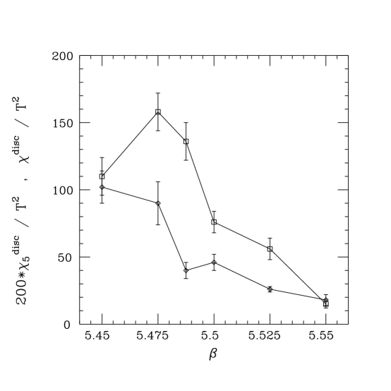
FIG. 3.: Disconnected susceptibilities as a function of $\beta$ ($N_{f}=2$,$ma=0.00625$).

To start with, we consider our results for the scalar and pseudoscalar susceptibilities. We separate the connected (i.e. volume integral of equations 4 or 5) and disconnected (i.e. volume integral of equations 14 or 15) contributions which are represented respectively as functions of $\beta$ in fig. 2 and fig. 3. We will first discuss the scalar susceptibility. Our results at $N_{t}=8$ are compatible with those of earlier works at $N_{t}=4$ [30], $N_{t}=6$ [31] and $N_{t}=12$ [32] . In particular, we find a peak in the disconnected but not in the connected susceptibility. It is important to note that if this situation were to persist in the chiral limit it would imply that only the flavor singlet scalar becomes massless at the transition and not the flavor triplet scalar. This would imply that the $U(1)$ axial symmetry remains broken at $T_{c}$. We will return to this discussion below. At a more technical level, we also find some slight differences with earlier works. For example, in the connected scalar susceptibility, we see a larger jump at the crossover than had been seen before. This is consistent with a rather abrupt change of the screening mass of the $\delta$ meson (see below), although the later effect is not statistically as significant. In the pseudoscalar channel, the most interesting behavior is related to the disconnected correlator. This is because of its association with topology through the integrated anomalous Ward identity:

$$m\int d^{4}x\bar{\psi}\gamma_{5}\psi=Q_{top}$$ (27)

on each gauge field configuration. Therefore, in the continuum, we would have:

$$m^{2}\chi_{5}^{dis}=\chi_{top}\equiv{<Q^{2}_{top}>\over V}$$ (28)

As we will see below, this relation doesn’t translate exactly to the lattice. However a remnant can be identified. We also note that the connected pseudoscalar susceptibility is almost constant accross the transition. This is in part a lattice artefact. In the continuum, we would expect that this susceptibility (equivalent to the flavor triplet pseudoscalar susceptibility) picks up a large contribution in the broken phase from the near masslessness of the pion in the chiral limit. This does not occur here because the lattice $\Gamma_{5}$ operator used above is not associated with a Goldstone pion in the staggered formulation.

FIG. 4.: Screening correlators at $\beta=5.4875$ ($N_{f}=2$,$ma=0.00625$).

FIG. 5.: Screening masses as a function of $\beta$ ($N_{f}=2$,$ma=0.00625$).

We now discuss the measurements of the screening masses. Because of large flavor symmmetry breaking, it is useful to separate the mesonic correlators into two categories: those corresponding to local operators and those corresponding to four link operators. In the first category, we have the pion (Goldstone) and the $\sigma$, to which we can add as well a representative of the $\vec{\delta}$ (connected part of the $\sigma$). Similarly, in the second category we would have the $\eta^{\prime}$ and $\vec{\delta}$ as well as a non-Goldstone pion (connected part of the $\eta^{\prime}$). In fig. 4 we show an example of correlators belonging to the first category at $\beta=5.4875$ (i.e. right above the crossover induced by the chiral phase transition). The screening masses extracted from our fits to those correlators as well as those measured at other values of $\beta$ are shown in fig. 5. The key feature of this plot is that the $\sigma$ becomes light close to the transition while the $\vec{\delta}$ remains heavy. This is what we would expect if the $U_{A}(1)$ symmetry were not restored at the chiral phase transition. It is also in agreement with the observation made earlier that the peak in the scalar susceptibility originates in the disconnected part of the correlator (see above). It is worth mentioning here that some of the fits leading to fig. 5 may have large systematic errors (only the statistical errors are included in the figure). This is due in part to the small extent of the lattice (and the use of point sources rather than “smearing improved” sources) and, in the case of the $\sigma$, to the additional difficulties associated with the measurements of disconnected quark loop correlators. Nevertheless, the qualitative picture emerging from fig. 5 appears rather clear: the $\sigma$ becomes lighter close to the transition while the $\vec{\delta}$ remains heavy. In fact, the trends observed in the early reports on this work [33] have been further confirmed by our recent addition of a “data point” at $\beta=5.4875$ . The main question that remains is the problem of the extrapolation to the chiral limit. Certainly, there are still rather large explicit chiral symmetry breaking effects in our current data ($ma=0.00625$) as can be seen from the fact that above the chiral phase transition ($m_{\sigma}-m_{\vec{\pi}}$) is almost as large as the $U_{A}(1)$ symmetry breaking ($m_{\vec{\delta}}-m_{\vec{\pi}}$). Measurements at lower values of the quark mass would therefore be needed to clarify the situation but are beyond the scope of this work. In addition, in section VI, we show that the issue of the chiral limit is rather subtle and requires a detailed understanding of at least some lattice artefacts. This implies in particular that a quantitative determination of the screening masses in the chiral limit will require the use of improved actions or very large lattices. In summary, the data shown in fig. 5 are suggestive of a situation where $U_{A}(1)$ is only restored at some $T>T_{c}$, but not sufficient by themselves to prove this fact. We will only achieve that goal after identifying the topological origin of the difference between the $\vec{\delta}$ and $\sigma$ propagators for small quark masses in the high temperature symmetric phase (see section VI). Finally, in fig. 6, we also present for completeness the screening masses obtained from the correlators involving four-link operators. These however are much less informative at the current values of $\beta$, since flavor symmetry breaking makes all the states heavy in this case. Note that fig. 6 is drawn to the same scale as fig. 5 but with a mass shift of $0.5$ along the vertical axis.

FIG. 6.: Screening masses in the channels associated with 4-link mesonic operators as a function of $\beta$ ($N_{f}=2$,$ma=0.00625$).

V Low lying fermionic modes and disconnected correlators

As was shown in section II, the presence of $U_{A}(1)$ symmetry breaking effects at $m=0$ in the $SU(2)_{L}\times SU(2)_{R}$ symmetric phase is equivalent to the existence of a non-zero disconnected contribution to flavor singlet correlators (compare formulae (21) and (22) for example). In addition, these contributions are accounted for entirely by exact fermionic zero-modes (13). An interesting way of studying $U_{A}(1)$ breaking in the chiral limit is therefore to compute the low lying eigenmodes of the Dirac operator. In this section, we compute the lowest 8 (positive) eigenvalues ($\lambda$) and the associated modes on each configuration of our sample at $ma=0.00625$ and discuss how close they are to satisfying the Atiyah-Singer index theorem and how well they already saturate the disconnected correlators. In the next section, we will see how the knowledge of these low modes can be used to extract information about the chiral limit. In both cases, the existence of the zero-mode shift lattice artefact [13] requires a detailed and careful analysis.

FIG. 7.: Eigenmode chirality versus $\lambda$ for the lowest 8 eigenvalues on each configurations of our quenched sample at $\beta=6.2$ .

FIG. 8.: Eigenmode chirality versus $\lambda$ for the lowest 8 eigenvalues on each configurations of our full QCD sample at $\beta=5.55$ .

We start by studying the disconnected susceptibilities (integrated correlators). For this purpose, we make use of the spectral decomposition of the quark propagator (3) and the resulting formulae:

$$Q\equiv TrS=\sum_{\lambda>0}{2m\over\lambda^{2}+m^{2}}+{n_{L}+n_{R}\over m}$$ (29)

$$Q_{5}\equiv Tr\gamma_{5}S={n_{L}-n_{R}\over m}$$ (30)

where $n_{L}(n_{R})$ are respectively the number of left (right) zero-modes of the Dirac operator. In terms of these, the scalar and pseudoscalar disconnected susceptibilities are defined as:

$$\chi^{dis}=[<Q^{2}>-(<Q>)^{2}]/V$$ (31)

$$\chi_{5}^{dis}=<Q^{2}_{5}>/V$$ (32)

FIG. 9.: Disconnected pseudoscalar susceptibilities as a function of $\beta$. Complete result (top curve) and truncation to the lowest 8 modes (bottom curve).

FIG. 10.: Disconnected scalar susceptibilities as a function of $\beta$. Complete result (top curve) and truncation to the lowest 8 modes (bottom curve).

Following the same reasoning as in section II, it is shown that in the continuum, $\chi_{(5)}^{dis}$ is completely saturated in the chiral limit by contributions from configurations with one zero-mode per flavor. On the lattice however this situation is not reproduced exactly. First there are no exact zero-modes (except on a subspace of measure 0). Then:

$$Q^{latt}=\sum_{\lambda>0}{2m\over\lambda^{2}+m^{2}}$$ (33)

$$Q_{5}^{latt}=\sum_{\lambda>0}{2m<\psi_{\lambda}|\Gamma_{5}|\psi_{\lambda}>\over\lambda^{2}+m^{2}}$$ (34)

where we have used the symmetries of the staggered action and $\Gamma_{5}$ is the (four-link) lattice $\gamma_{5}$ operator. It is then clear that in the current lattice formulation, disconnected susceptibilities will vanish in the chiral limit and be proportional to $m^{2}$ for small $m$. This is a direct consequence of the zero mode shift lattice artefact [13]. Incidently, we believe that it is this artefact which makes an extrapolation from lattice data extremely difficult [11, 12]. In view of this situation, it is important that we study how much of the continuum behavior is already visible in the lattice data. Clearly, a corner stone is the Atiyah-Singer index theorem, namely the relation between topology and the existence of chiral fermionic zero-modes. Formula (30) in particular comes about because in the continuum $<\psi_{\lambda}|\gamma_{5}|\psi_{\lambda}>$ is either $\pm 1$ if $\lambda=0$ or $0$ otherwise. The lattice expression (34) will closely match the continuum if we see on the lattice a clear correlation between small eigenvalues and large $r_{\lambda}\equiv<\psi_{\lambda}|\gamma_{5}|\psi_{\lambda}>$ (i.e. if we can identify chiral modes). These correlations can be studied by drawing a plot of $r_{\lambda}$ versus $\lambda$ for all (low lying) eigenvalues associated with our configuration sample (as was done by Hands and Teper in a zero temperature SU(2) Yang-Mills theory [34]). Here we present two examples of such plots. Fig. 7 was obtained on our sample of quenched configurations at $\beta=6.2$, while fig. 8 presents the same results in the case of 2 flavor QCD at $\beta=5.55$. In each case, we have tried to identify the topology of the gauge field configurations by cooling and have used different symbols to represent eigenvalues obtained on configurations with different $Q_{cool}$ (see insert in fig. 7 and 8). The correlation between large $r_{\lambda}$ and small $\lambda$ is visible on fig. 8 and very clear on fig. 7. As expected, our computations at other values of $\beta$ indicate that both for quenched and full QCD the correlations deteriorate as one moves towards stronger coupling. Note that, the relatively low value of $r_{\lambda}$ ( $\sim 0.20$ in fig. 7 and $<0.10$ in fig. 8) compared with the continuum value of $1.0$ follows from large renormalisation of the pseudoscalar operator (This is to be expected since $\Gamma_{5}$, being a 4-link operator, picks up a large correction factor even in the mean-field approximation). With the knowledge of the eigenvalues and of $r_{\lambda}$, we can compute the disconnected susceptibilities from the formulae (31-32) and (33-34) (in our case truncated to the lowest 8 modes). The susceptibilities obtained in this way are compared in fig. 9 and 10 with those computed with a noisy estimator in section IV. In the case of the pseudoscalar disconnected susceptibility (fig. 9), excellent agreement is obtained at $\beta=5.55$ and reasonable agreement in the rest of the symmetric phase. A similar situation is obtained for the scalar susceptibilities (fig. 10). The agreement is not expected to be as good there however since, even in the continuum, the explicit symmetry breaking ($ma=0.00625$ in our case) implies a sensitivity to higher eigenvalues (see (29)) and dominance by the low lying modes is only expected to be recovered very close to the chiral limit.

Overall, we conclude that in spite of lattice artefacts, the ingredients for a breaking of $U_{A}(1)$ symmetry according to the scenario described in section II are present in our simulations at finite quark mass. In particular, we have shown evidence for the existence of topological fermionic zero-modes and have shown that these low lying modes are already accounting for a large part of the disconnected susceptibilities. In the next section, we will complete the argument by showing that the $U_{A}(1)$ symmetry breaking indeed survives in the chiral limit once the zero-mode shift lattice artefact is corrected for.

Finally, it is interesting to note that not only the susceptibilities but the entire disconnected correlators themselves are dominated by the low lying modes. In fig. 11 ,we compare the pseudoscalar disconnected correlator at $\beta=5.55$ obtained in this way with the one computed with a noisy estimator. Again excellent agreement is found. Certainly, it would be interesting to study the nature of those eigenmodes in greater details and for example their properties of localization (around instantons?).

FIG. 11.: Comparison of the disconnected pseudoscalar correlators obtained from a noisy estimator (top curve) and from the truncated spectral decomposition of the quark propagator (bottom curve) at $\beta=5.55$ ($N_{f}=2$,$ma=0.00625$).

VI Chiral limit

FIG. 12.: Pseudoscalar disconnected susceptibility as a function of quark mass: (a) At $\beta=6.2$, in a partially unquenched approach with 0 to 8 modes included in the fermionic determinant (from top to bottom). (b) Same as (a) but with the Atiyah-Singer index theorem enforced “by hand”. (c) At $\beta=5.55$, using a reweighting by partial determinants to compute the mass dependance, with 0 to 8 modes included (from top to bottom). (d) Same as (c) but with the Atiyah-Singer index theorem enforced “by hand”.

In section V, we showed that the value of $\chi_{5}^{dis}$ at $ma=0.00625$ and $\beta=5.55$ could be entirely understood from the knowledge of the lowest 8 eigenvalues/eigenvectors of the Dirac operator on each gauge configuration of our sample. Since the saturation of this quantity by low lying modes will be even better at lower values of the quark mass (as can be seen from (34)), this result can be used to investigate the chiral limit.

At first, we consider a “partially quenched approach” where the value of the quark mass in the fermionic determinant is kept fixed at a value which we shall call $m_{0}$ (in our case $am_{0}=0.00625$) while a varying mass $m$ is introduced in the quantity we measure. A similar approach was taken in ref. [12]. Since low mode dominance was obtained at $am_{0}=0.00625$, $\chi_{5}^{dis}$ can be computed from (34) for all $m\leq m_{0}$. The $m$ dependance of $\chi_{5}^{dis}$ obtained in this way is presented in fig. 12.c (top curve). The result depends sensitively on $m$ and vanishes at $m=0$, as expected from the zero-mode shift phenomenon (If there were exact zero-modes,the result would diverge like $1/m^{2}$). It is also easy to show that $\chi_{5}^{dis}$ will remain zero at $m=0$ in the unquenched case. For this purpose, we introduce partial determinants:

$$\Delta_{k}(m)=[\prod_{n=1}^{k}(\lambda_{n}^{2}+m^{2})]^{N_{f}/4}$$ (35)

Successive approximations to the full QCD result are obtained by introducing the reweighting factor $[\Delta_{k}(m)/\Delta_{k}(m_{0})]$ in our measurements (The exact answer is then obtained for $k\rightarrow k_{max}$). Fig. 12.c presents the results obtained in this way for k=0 to 8 (from top to bottom). The error bars are omitted for the clarity of the figure. In fig. 13.c, we present the result of applying the same procedure in the case of the disconnected scalar susceptibility. Since there is no complete dominance of $\chi^{dis}$ by the lowest 8 modes (see fig. 10) the curves in fig. 13.c are only qualitative in character (as opposed to those of fig. 12 which are quantitative). Quantitative details, however, will not be important in the discussion given below. What is important here is that $\chi^{dis}$ (like $\chi_{5}^{dis}$) vanishes in the chiral limit (although maybe with a slightly different approach to zero).

FIG. 13.: Scalar disconnected susceptibility as a function of quark mass: (a) At $\beta=6.2$, in a partially unquenched approach with 0 to 8 modes included in the fermionic determinant (from top to bottom). (b) Same as (a) but with the Atiyah-Singer index theorem enforced “by hand”. (c) At $\beta=5.55$, using a reweighting by partial determinants to compute the mass dependance, with 0 to 8 modes included (from top to bottom). (d) Same as (c) but with the Atiyah-Singer index theorem enforced “by hand”.

If taken at face value, the lattice measurements described in fig. 12.c and fig. 13.c would imply that the $U_{A}(1)$ symmetry is restored at $\beta=5.55$. However, we will argue that this result is the consequence of a lattice artefact and therefore misleading. In particular, we show below that the vanishing of the disconnected susceptibilities in the chiral limit is a result of the zero mode shift phenomenon. To do this, we turn to our quenched measurements at $\beta=6.2$ where the smoothness of the gauge field allows us to make the argument even clearer. In particular, the topology of a gauge field configuration can be almost unambiguously determined in this case. Since we are now starting from quenched configurations, the reweighting occurs through the partial determinants $\Delta_{k}$ and a “k modes” approximation to the average of an operator $A$ is given by:

$$\langle A\rangle_{k}=\int{D}Ue^{-S_{G}}\Delta_{k}(m)A/Z_{k}$$ (36)

$$Z_{k}=\int{D}Ue^{-S_{G}}\Delta_{k}(m)$$ (37)

The results obtained for the pseudoscalar and scalar disconnected susceptibilities as functions of quark mass are represented in figs. 12.a and 13.a respectively. Again the disconnected susceptibilities vanish in the chiral limit (for any k). However, since topology can be easily identified in this case, it is possible to attempt to correct for the zero mode shift lattice artefact. We will in fact enforce the Atiyah-Singer index theorem “by hand” by replacing the first $2Q_{top}$ eigenvalues by $\lambda=0$ . After this correction is applied, the disconnected susceptibilities become very smooth functions of the quark mass, which extrapolate to non-zero values (figs. 12.b and 13.b). Of course, the current approach is still partially quenched (with only up to 8 fermionic modes included in fig. 12.b and 13.b) while the inclusion of the full fermionic determinant might make the disconnected susceptibilities (vanishingly) small at $\beta=6.2$. However, the point that we want to make here is about the smoothness of the chiral limit, i.e. correcting for the zero-mode shift lattice artefact has allowed us to get around the otherwise apparently unavoidable consequence of a vanishing chiral limit (see fig. 12.a and 13.a). A similar discussion can be given for the case of full QCD at $\beta=5.55$, the only difference is that the determination of the topological charge of gauge field configurations is now more difficult because of the lower value of $\beta$. Qualitatively however, the results (12.d and 13.d) are the same as shown above. Although the chiral limits obtained after “correction” are only rough estimates (see fig. 12.d and 13.d), it is clear that the disconnected susceptibilities at $m=0$ are different from 0 (once the Atiyah-Singer index theorem is properly taken into account). In other words, the $U_{A}(1)$ axial symmetry is not restored even at $\beta=5.55$ (which corresponds to a temperature well above the critical temperature of the $SU(2)_{L}\times SU(2)_{R}$ symmetry restoration) ! The question of how large exactly the $U_{A}(1)$ symmetry breaking is (as a function of $T$ at $m=0$), however, is beyond the scope of this paper. The quantitative determination of the size of the symmetry breaking can only be addressed by using much larger lattices and weaker coupling or through the use of improved actions which better satisfy the Atiyah-Singer index theorem. Many recently introduced ideas need to be tested in this respect. In this paper, we only take a modest first step by analyzing the case of the “fat link” improved quark action [39] in section VII. Other formulations which are currently under test include the “perfect action” approach [36] and the domain wall fermion formulation (DWF) [37]. Some encouraging results were obtained recently for DWF in the context of QED in 2 dimensions [41]. It is also worth mentioning that dynamical Wilson fermions would not suffer from the “vanishing problem” in the chiral limit. There the zero-modes are shifted along the real axis and multiplication by the fermionic determinant ensures a smooth behavior. The role of DWF in this context is then to give a “global” (i.e. valid on all configurations at the same time) definition of the quark mass (and in particular of the point $m_{q}=0$). Let us also mention that improved gauge actions would also help in so far as they sample configurations with smoother short distance behavior on which the Atiyah-Singer index theorem is better satisfied.

Finally, it is important to remember that in this paper, the issue of the $U_{A}(1)$ symmetry restoration is studied only at a single value of the spatial volume, namely $V=(2/T)^{3}$. The actual volume dependance of our results remains to be investigated.

VII Improvement of the staggered fermionic action

FIG. 14.: Eigenmode chirality versus $\lambda$ using a “fat-link” improved quark action on our quenched $\beta=6.2$ gauge field configurations.

All of the results presented above clearly indicate the importance of finding improved quark actions which better satisfy the Atiyah-Singer index theorem. As already mentioned, there are many different methods which need to be tested. These range from the traditional improvement of the staggered [43] and Wilson [44] fermionic action to the study of perfect actions [36] and the domain wall fermion formulation [37, 38]. That is obviously a vast program and in this paper we will limit our attention to a discussion of the simplest modification of the staggered action used above. The idea is to investigate whether the methods proposed recently to improve the flavor symmetry properties of the staggered action [39, 40] also help in reducing the shift of the topological zero-modes. A priori, one would expect that the two phenomena are related. Indeed, the continuum limit of the staggered theory describes 4 quark flavors, which implies a 4-fold degeneracy of the eigenvalue spectrum in this limit. As one moves towards stronger coupling, the degeneracy is lifted and flavor symmetry breaking follows. Similarly, if there are zero modes in the continuum, these will be split too on the lattice. Therefore, in both cases improvement should be obtained by reducing the amount by which the eigenvalues are scattered. Recently, it was shown through measurements of $m^{2}_{\pi_{2}}-m^{2}_{\pi}$ that “fat-link” actions reduce the flavor symmetry breaking [39, 40]. Certainly it would be interesting to see how these actions modify the eigenvalue spectrum. In fig. 7 and 14, we compare the eigenvalue spectrum and pseudoscalar residue $r_{\lambda}\equiv\langle\psi_{\lambda}|\Gamma_{5}|\psi_{\lambda}\rangle$ for an ensemble of quenched configurations at $\beta=6.2$ on a $(16)^{3}\times 8$ lattice. Figure 7 corresponds to the usual staggered action, figure 14 corresponds to a “link+staples” model where each staple carries a relative weight of $1/2$ with respect to the link. (This action belongs to the category considered in [39]). We chose a relatively high value of $\beta$ (in the symmetric high temperature phase) so that topology could be easily identified. The symbols used in the plot correspond to the topological charge of each configuration (as determined by cooling). 8 modes have been computed per configuration. The most noticeable feature in these two plots is associated with the cluster of 4 eigenvalues which is seen close to the origin in fig. 14. Those eigenvalues come from a single configuration and should be interpreted as representing a mode with low eigenvalue but zero chirality (as expected on a configuration with zero topological charge). In the continuum, those 4 eigenvalues would be degenerate and $r_{\lambda}$ would be 0. With the standard staggered action (fig. 7) these 4 eigenvalues are much more dispersed and some even pick up a relatively large value of $r_{\lambda}$. So in this case, the improved action is clearly doing it’s job: it significantly reduces the flavor symmetry breaking. It is also interesting to note that the eigenvalues just discussed are of the type that would lead to chiral symmetry breaking once they condense . Typically they are of order $1/V$, and since they are small but not exactly zero, they are also non-chiral (i.e. $r_{\lambda}=0$). The other type of modes that we want to discuss are the chiral modes. In figures 7 and 14, these are the modes with $r_{\lambda}$ of the order of 0.15 or larger. These are associated with configurations with non-trivial topology and in the continuum would have $\lambda=0$. In order to preserve the distinction between the two types of modes and to ensure better properties of the chiral limit what we would at least require is that on a lattice (of finite volume) the eigenvalues of the chiral modes remain smaller than those of the non-chiral modes (which can be $O(1/V)$ when the chiral symmetry is broken). As can be seen on fig. 14, this is not yet realized at this stage. In other words, the “fat link” action doesn’t necessarily bring the chiral modes much closer to $\lambda=0$ compared to what it does on other modes. The situation can be summarized by saying that this type of improvement only corrects the largest flavor symmetry violation. It brings together eigenvalues which were widely separated before but does little on the others. In fact, the separation that remains between the four low modes on figure 14 is of the same order as the zero mode shift of chiral modes. Correcting those two effects could therefore only be achieved at a higher level of improvement. At the same time, other methods of improvements such as domain wall fermions and perfect actions should also be considered. It is quite conceivable that a combination of various methods may be necessary in the end.

VIII Summary and conclusions

We have shown that important insight can be gained about the flavor singlet dynamics of finite temperature QCD by computing the low lying modes of the Dirac operator. This follows from the simple result, derived in section II, that in the high temperature symmetric phase at finite volume, the scalar and pseudoscalar disconnected correlators are entirely accounted for by the contributions of fermionic zero-modes. Therefore, $U_{A}(1)$ symmetry breaking (i.e. the non-vanishing of the disconnected correlator) is directly linked through the Atiyah-Singer index theorem, to contributions from the sector of topological charge one in the functional integral.

This simple observation also warns us of possible difficulties with the lattice approach, since topological properties are often not very well reproduced in this context. In the case of a staggered quark action, used in this paper, the zero-mode shift lattice artefact implies that great care has to be taken in examining the chiral limit. That there are difficulties in extrapolating to $m_{q}=0$ was already known from the works of refs. [11, 12] where it was shown that it is extremely difficult to decide between linear and quadratic fits to the data. Here we have gone one step further and have shown that the disconnected susceptibilities must vanish in the chiral limit (possibly with a rather complicated approach) as a consequence of the zero-mode shift phenomenon.

Our computations also forced us to recognize this apparent restoration of $U_{A}(1)$ as a lattice artefact. In section V, for example, we have seen that our simulations indeed contain configurations with non-trivial topological charge and that associated with these are eigenstates with relatively large chirality and small eigenvalues. The main source of difficulties is that these eigenvalues are just small and not exactly zero as would be required by the Atiyah-Singer theorem, nor are they so small that they can be unambiguously separated from the other eigenvalues which would not vanish in the continuum limit. In fact, when we imposed the index theorem “by hand” and forced those eigenvalues to vanish, we found a smooth chiral limit and disconnected susceptibilities different from zero in the chiral limit (see section VI). This leads us to the conclusion that the $U_{A}(1)$ symmetry is not restored at $T_{c}$ but only at a somewhat higher (possibly infinite) temperature. At this point however this is still a qualitative conclusion. Quantitative questions such as the issue of exactly how large the symmetry breaking is as a function of temperature will only be addressable in the context of improved actions or very large lattices. There is therefore an urgent need for studies of lattice fermion formulations which better satisfy the Atiyah-Singer index theorem.

In this paper, we have taken a modest first step towards investigating improved actions by looking at the case of the “fat-link” formulation [39]. This technique has been shown to lessen the flavor symmetry breaking in the mesonic spectrum. For our purposes however, we have seen in section VII, that the improvement that it provides at the level of the eigenvalue spectrum is too small to make a big difference in the identification of topological zero-modes.

Beyond this, there is much more that can be done from the knowledge of the low lying eigenvalues and eigenvectors computed in this paper. The spectrum itself and the distribution of eigenvalues could be compared with random matrix models [45]. Since we also have the eigenvectors, their properties of localization possibly around instantons or other objects could be investigated as well. In the context of finite temperature, many interesting questions related to the change of properties of the instanton medium, the possible existence of instanton + anti-instanton molecules [46], and their relation to quark probes deserve to be studied.

When some of the issues discussed above are settled, it will also be quite important to study several physical volumes rather than just $V=(2/T)^{3}$ as was done here. The fact that we have identified topological effects and a $U_{A}(1)$ symmetry breaking in a relatively small volume doesn’t necessarily mean that this will survive in the infinite volume limit: The nature of topological fluctuations might depend significantly on the volume.

IX ACKNOWLEDGEMENTS

This work was supported by the U. S. Department of Energy under contract W-31-109-ENG-38, and the National Science Foundation under grant NSF-PHY92-00148. The computations were performed on the CRAY C-90 at NERSC. We would like to thank Carleton DeTar and Edwin Laermann for informative conversations and the HTMCGC collaboration for the use of their configurations.

REFERENCES

- [1] A. Ukawa, Nucl. Phys. B(Proc. Suppl.) 53, 106 (1997).
- [2] C. DeTar, in ’Quark Gluon Plasma 2’, edited by R. Hwa, World Scientific, 1995.
- [3] F. Karsch, Lectures given at the “Enrico Fermi School” on Selected Topics in non perturbative QCD, 27 June - 7 July 1995, Varenna, Italy.
- [4] J. B. Kogut and D. K. Sinclair, Nucl. Phys. B(Proc. Suppl.) 53, 272 (1997).
- [5] R. Pisarski and F. Wilczek, Phys. Rev. D 29, 338 (1984).
- [6] E. Shuryak, Comments Nucl. Part. Phys. 21, 235 (1994).
- [7] T. D. Cohen, Phys. Rev. D 54, 1867 (1996).
- [8] S. H. Lee and T. Hatsuda, Phys. Rev. D 54, 1871 (1996).
- [9] N. Evans, S. D. H. Hsu and M. Schwetz, Phys. Lett. B 375, 262 (1996).
- [10] G. Boyd, F. Karsch, E. Laermann, M. Oevers, hep-lat/9607046, talk given at 10th International Conference on Problems of Quantum Field Theory, Alushta, Ukraine, 13-17 May 1996.
- [11] C. Bernard et al., Phys. Rev. Lett. 78, 598 (1997).
- [12] S. Chandrasekharan and N. H. Christ, Nucl. Phys. B (Proc. Suppl.) 47 (1996) 527; N. Christ, Nucl. Phys. B (Proc. Suppl.) 53 (1997) 253; A. Kaehler, hep-lat/9709141, talk given at Lattice 97: 15th International Symposium on Lattice Field Theory, Edinburgh, Scotland, 1997.
- [13] J. C. Vink, Phys. Lett. 210 B (1988) 211.
- [14] H. Joos and S. I. Azakov, Helv. Phys. Acta 67, 723 (1994).
- [15] J. Kapusta, D. Kharzeev and L. McLerran, Phys. Rev. D 53, 5028 (1996).
- [16] Z. Huang and X.-N. Wang, Phys. Rev. D 53, 5034 (1996).
- [17] T. Schafer, Phys. Lett. B 389, 445 (1996).
- [18] T. Hatsuda and T. Kunihiro, Phys. Rep. 247 (1994) 221.
- [19] S. Coleman, Comm. Math. Phys. 31 (1973) 259.
- [20] A. Smilga and J. J. M. Verbaarschot, Phys. Rev. D 54, 1087 (1996)
- [21] A. V. Smilga, Phys. Rev. D 55, 443 (1997).
- [22] S. Gottlieb et al., Phys. Rev. D 55, 6852 (1997).
- [23] T. Blum, L. Kärkkäinen, D. Toussaint and S. Gottlieb, Phys. Rev. D 51, 5153 (1995).
- [24] G. Kilcup, J. Grandy and L. Venkataraman, Nucl. Phys. B (PS), 47 (1996) 358.
- [25] L. Venkataraman and G. Kilcup, hep-lat/9711006
- [26] T. Kalkreuter and H. Simma, Comput. Phys. Commun. 93, 33 (1996).
- [27] B. Bunk, Nucl. Phys. (Proc. Suppl.) 53 (1997) 987.
- [28] D. Sorensen, SIAM J. Matrix Anal. Appl. 13, 357 (1992).
- [29] T. L. Ivanenko and J. W. Negele, hep-lat/9709130, talk given at Lattice 97: 15th International Symposium on Lattice Field Theory, Edinburgh, Scotland, 1997.
- [30] F. Karsch and E. Laermann, Phys. Rev. D 50, 6954 (1994).
- [31] C. Bernard et al., Phys. Rev. D 45, 3854 (1992). T. Blum et al., Phys. Rev. D 51, 5153 (1995); C. Bernard et al., Phys. Rev. D 55, 6861 (1997).
- [32] C. Bernard et al., Phys. Rev. D 54, 4585 (1996).
- [33] J. B. Kogut, J.-F. Lagae and D. K. Sinclair, Nucl. Phys. B(Proc. Suppl.) 53, 269 (1997).
- [34] S. J. Hands and M. Teper, Nucl. Phys. B 347, 819 (1990).
- [35] W. Bardeen et al., hep-lat/9705008.
- [36] P. Hasenfratz, hep-lat/9709110, Plenary talk given at Lattice’97: 15th International Symposium on Lattice Field Theory, Edinburgh, Scotland, 1997.
- [37] Y. Shamir, Nucl. Phys. B 406 (1993) 90.
- [38] R. Narayanan and P. Vranas, Nucl. Phys. B 506, 373 (1997).
- [39] T. Blum et al., Phys. Rev. D 55, R1133 (1997).
- [40] J.-F. Lagae and D. K. Sinclair, hep-lat/9709067, talk given at Lattice 97: 15th International Symposium on Lattice Field Theory, Edinburgh, Scotland, 1997.
- [41] P. M. Vranas, hep-lat/9705023.
- [42] S. Itoh, Y. Iwasaki and T. Yoshie, Phys. Rev. D 36, 527 (1987).
- [43] S. Naik, Nucl. Phys. B. 316, 238 (1989).
- [44] B. Sheikholeslami and R. Wohlert, Nucl. Phys. B259, 572 (1985).
- [45] J. B. Kogut, J.-F. Lagae and D. K. Sinclair, work in progress.
- [46] T. Schafer, E. V. Shuryak and J. J. M. Verbaarschot, Phys. Rev. D 51, 1267 (1995).