Statistical properties at the spectrum edge of the QCD Dirac operator

Abstract

The statistical properties of the spectrum of the staggered Dirac operator in an SU(2) lattice gauge theory are analyzed both in the bulk of the spectrum and at the spectrum edge. Two commonly used statistics, the number variance and the spectral rigidity, are investigated. While the spectral fluctuations at the edge are suppressed to the same extent as in the bulk, the spectra are more rigid at the edge. To study this effect, we introduce a microscopic unfolding procedure to separate the variation of the microscopic spectral density from the fluctuations. For the unfolded data, the number variance shows oscillations of the same kind as before unfolding, and the average spectral rigidity becomes larger than the one in the bulk. In addition, the short-range statistics at the origin is studied. The lattice data are compared to predictions of chiral random-matrix theory, and agreement with the chiral Gaussian Symplectic Ensemble is found.

1 Introduction

The spectrum of the Dirac operator is an important aspect of nonperturbative QCD. In Euclidean space, the Dirac operator reads $i\hbox{\large$/$}\kern-7.27847pt\hbox{$D$}=i\hbox{\large$/$}\kern-5.65451pt\hbox{$\partial$}+g(\lambda^{a}/2)\hbox{\large$/$}\kern-6.75pt\hbox{$A$}^{a}$, where $g$ is the coupling constant, $\lambda^{a}$ are the generators of SU($N$)-color, and $A_{\mu}^{a}$ are the gauge fields. Whether in the continuum or on the lattice, to obtain physical observables one has to perform an average over the ensemble of gauge field configurations. The eigenvalues of $i\hbox{\large$/$}\kern-7.27847pt\hbox{$D$}$ fluctuate over this ensemble of gauge fields. In many areas of physics, e.g., in classically chaotic systems, complex nuclei, and disordered mesoscopic systems, the study of energy level statistics plays a prominent role. Although the global spectral fluctuations are strongly system dependent, the local spectral correlations on the scale of the mean level spacing are universal and only depend on the global symmetries of the system under consideration. These universal correlations can be obtained exactly in random-matrix theory (RMT) Bohi84 . In order to describe the universal statistical properties of the eigenvalues of $i\hbox{\large$/$}\kern-7.27847pt\hbox{$D$}$, one needs random-matrix models which take the chiral symmetry of the Dirac operator into account Shur93 . In a chiral random-matrix model, the matrix of the Dirac operator (in a chiral basis in Euclidean space) is replaced by a random matrix $W$ with appropriate symmetries,

$$i\hbox{\large$/$}\kern-7.27847pt\hbox{$D$}\rightarrow\left[\matrix{0&W\cr W^{\dagger}&0}\right]\;.$$ (1)

The average over gauge fields is replaced by an average over the ensemble of random matrices, and the gluonic part of the weight function, $\exp(-S_{\rm gl})$, is replaced by a simple Gaussian distribution of the random matrix $W$. Depending on the number of colors and the representation of the fermions, the Dirac operator falls into one of three universality classes which were classified in Ref. Verb94a and correspond to the three chiral Gaussian random-matrix ensembles. These are the chiral Gaussian orthogonal (chGOE), unitary (chGUE), and symplectic (chGSE) ensemble in which the random matrix $W$ is either real, complex, or quaternion real, respectively. For a recent review of important results, we refer to Ref. Verb97 .

Various quantities, in addition to the spectral correlation functions, have been employed to describe the statistical properties of the spectrum of a given system. One uses the number variance and the spectral rigidity, to be defined below, to measure long-range correlations, whereas the distribution of spacings between eigenvalues is used to probe short-range correlations in the spectrum. A statistical analysis of the spectrum of the Dirac operator was first performed using data obtained by Kalkreuter in an SU(2) lattice gauge theory with both Wilson and Kogut-Susskind fermions Hala95 , and it was found that the lattice data were described by RMT. Recently, high-statistics lattice data obtained by Berbenni-Bitsch and Meyer were analyzed. Again, perfect agreement with RMT was found Wilk97 . In the bulk of the spectrum, the local spectral fluctuation properties follow the predictions of the conventional Gaussian ensembles, which in this case are identical to those of the chiral ensembles Naga91 .

The QCD Dirac operator has a special symmetry which has important implications for the edge of the spectrum. Since the Dirac operator anti-commutes with $\gamma_{5}$, its eigenvalues appear in pairs $\pm\lambda$ leading to level repulsion at $\lambda=0$. Based on an analysis of Leutwyler-Smilga sum rules Leut92 , Shuryak and Verbaarschot Shur93 conjectured that the so-called microscopic spectral density of the Dirac operator, defined by

$$\rho_{s}(z)=\lim_{V\to\infty}\frac{1}{V\Sigma}\;\rho\left(\frac{z}{V\Sigma}\right)\;,$$ (2)

should be a universal quantity as well. Here, $\rho(\lambda)=$$\langle\sum_{i}\delta(\lambda-\lambda_{i})\rangle_{A}$ is the overall spectral density of the Dirac operator, $V$ is the space-time volume, and $\Sigma$ is the absolute value of the chiral condensate, respectively. According to the Banks-Casher formula, $\Sigma=\pi\rho(0)/V$ Bank80 , the spectral density at zero virtuality is proportional to the chiral condensate, therefore the spectrum edge is of great interest for the understanding of the spontaneous breaking of chiral symmetry in QCD. The definition of Eq. (2) leads to a magnification of the region of small eigenvalues by a factor of $V\Sigma$, thus the microscopic spectral density also provides information about the approach to the thermodynamic limit.

If $\rho_{s}$ is a universal quantity, it should also be calculable in chiral random-matrix theory (chRMT). This was done for all three chiral ensembles in the chiral limit Verb93 ; Verb94c ; Naga95 . Several pieces of evidence have lent support to the universality conjecture for $\rho_{s}$. We mention here the reproduction of Leutwyler-Smilga sum rules Verb93 , the microscopic spectral density in an instanton liquid model Verb94b , the valence quark mass dependence of the chiral condensate Chan95 ; Verb96a , theoretical universality proofs with regard to the probability distribution of the random matrix Brez96 ; Nish96 ; Slev93 , and finite temperature calculations Jack96b . Very recently, the conjecture was verified directly by lattice calculations. In Ref. Berb97a , the microscopic spectral density, the distribution of the smallest eigenvalue, and the microscopic two-point correlator were constructed from lattice data calculated by Berbenni-Bitsch and Meyer for an SU(2) gauge theory with staggered fermions in the quenched approximation and compared with the random-matrix predictions. The agreement was excellent.

Another very interesting area of application of chiral random-matrix theory is the construction of schematic models for the chiral phase transition at finite temperature and/or chemical potential Jack96a ; Wett96 ; Step96a ; Step96b ; Nowa96 ; Jani97a ; Hala97a ; Hala97b . It should be emphasized that while chRMT yields exact results for the spectral correlations in the bulk of the spectrum and at the spectrum edge, the results of these schematic models typically are not universal. Nevertheless, such models can shed light on a number of important issues, such as the nature of the quenched limit at finite chemical potential Step96b . Other aspects concern the relation with Nambu–Jona-Lasinio models Jani97a and the U_A(1) problem Jani97b . In this paper, however, we shall not discuss such models but concentrate on the universal properties of the spectrum of the Dirac operator.

It is the goal of the present work to perform the statistical spectral analysis at the spectrum edge for the same lattice data as in Ref. Berb97a and to compare to the statistical properties in the bulk. Our aim is two-fold: (i) to test, for higher order correlations, the conjecture that the spectral statistics of the QCD Dirac operator are universal and described by chRMT, and (ii) to gain an intuitive understanding of the statistical properties of the Dirac spectra at the edge (at zero virtuality). The difference between the usual situation (normally in the spectrum bulk) and the present one is the hard edge at $\lambda=0$ which breaks the translational invariance of the spectrum in this region.

In Sec. 2 we give, for the microscopic region, the theoretical predictions for the one- and two-point spectral correlation functions of the chGSE and the expressions for the number variance and the average spectral rigidity applicable to the present situation. Section 3 is devoted to the analysis of lattice data with regard to the long-range statistics, as well as the one- and two-point correlation functions. We then perform, in Sec. 4, a microscopic unfolding in order to obtain a better understanding of the behavior of the long-range correlations obtained in Sec. 3. In Sec. 5 we study the spacing distribution in a specific case. The last section is a summary and also discusses the effect of lattice parameters on our results.

2 Theoretical predictions of the chGSE

The appropriate ensemble corresponding to staggered fermions in SU(2) is the chGSE Verb94a . A central object in RMT is the joint distribution function of the eigenvalues of the matrix in Eq. (1) which is obtained after diagonalizing the matrix and computing the Jacobian. If $W$ has $N+\nu$ rows and $N$ columns, then the matrix in (1) has $N$ positive eigenvalues $\lambda_{1},\ldots,\lambda_{N}$, $N$ negative eigenvalues $-\lambda_{1},\ldots,-\lambda_{N}$, and $\nu$ zero modes (we assume $\nu\geq 0$). The joint distribution function then reads Verb94a

$$P(\lambda_{1},\ldots,\lambda_{N}) \sim \prod_{j=1}^{N}\lambda_{j}^{2N_{f}+4\nu+3}e^{-2N\Sigma^{2}\lambda_{j}^{2}}\prod_{k<l}^{N}(\lambda_{k}^{2}-\lambda_{l}^{2})^{4}\;,$$

where we have omitted a normalization factor which ensures that $\int d\lambda_{1}\cdots d\lambda_{N}\rho=1$. Here, $N_{f}$ is the number of massless flavors, and $\nu$ corresponds to the topological charge. For the quenched lattice data we consider, $N_{f}=0$ and $\nu=0$.

We now need expressions for the scaled one- and two-point functions at the spectrum edge. They can be derived from results computed by Nagao and Forrester Naga95 for the Laguerre ensemble with the joint distribution function

$$P(x_{1},\dots,x_{N})\sim\prod_{j=1}^{N}x_{j}^{4a}e^{-4x_{j}}\prod_{k<l}^{N}(x_{k}-x_{l})^{4}$$ (4)

by a simple transformation of variables, $4x=2N\Sigma^{2}\lambda^{2}$. Evidently, $4a=N_{f}+2\nu+1$. We use the same letter $P$ to denote the joint distribution functions (2) and (4). For convenience, we introduce a new parameter

$$\mu=N_{f}+2\nu$$ (5)

which will characterize the dependence of the various quantities we consider on $N_{f}$ and $\nu$. For the present lattice data we have $\mu=0$. The $k$-point function follows by integrating the joint distribution function over all but $k$ variables,

$$R_{k}(\lambda_{1},\ldots,\lambda_{k}) =$$ (6)

$$\frac{N!}{(N-k)!}\int\cdots\int d\lambda_{k+1}\cdots d\lambda_{N}P(\lambda_{1},\ldots,\lambda_{N})\;.$$

A note on notation: We denote the usual $k$-point functions by $R_{k}$ and the corresponding microscopic limits by $\rho_{k}$. The microscopic limit of the $k$-point function is obtained by rescaling all arguments by a factor of $2N\Sigma$ in analogy with Eq. (2). Setting the lattice constant to unity, we can identify the volume $V$ with the number of eigenvalues $2N+\nu\approx 2N$ in the large-$N$ limit. Including the proper normalization and using the result of Ref. Naga95 , we obtain for the microscopic one-point function

$$\rho_{s}(z) = \lim_{N\to\infty}\frac{1}{2N\Sigma}R_{1}\left(\frac{z}{2N\Sigma}\right)$$ (7)

$$= 2z^{2}\int_{0}^{1}duu^{2}\int_{0}^{1}dv[J_{\mu}(2uvz)J_{\mu+1}(2uz)$$

$$\phantom{2z^{2}\int_{0}^{1}duu^{2}\int_{0}^{1}}-vJ_{\mu}(2uz)J_{\mu+1}(2uvz)]\;,$$

where $J$ denotes the Bessel function. Asymptotically, $\rho_{s}(z)$ $\to 1/\pi$ as $z\to\infty$. To compare with the bulk properties, it is convenient to rescale the argument by a factor of $\pi$ so that it is measured exactly in terms of the local mean level spacing. (This factor of $\pi$ comes in through the Banks-Casher relation, $\Sigma=\pi\rho(0)/V$.) The result in Eq. (7) can be simplified further and expressed in terms of a single integral Berb97b . We obtain after some algebra

$$\rho_{1}(z) = \pi\rho_{s}(\pi z)$$ (8)

$$= \pi^{2}z[J_{\mu}^{2}(2\pi z)-J_{\mu+1}(2\pi z)J_{\mu-1}(2\pi z)]$$

$$-\frac{\pi}{2}J_{\mu}(2\pi z)\int_{0}^{2\pi z}dtJ_{\mu}(t)\;.$$

The two-point spectral correlation function is given by

$$R_{2}(\lambda_{1},\lambda_{2})=R_{1}(\lambda_{1})R_{1}(\lambda_{2})-T_{2}(\lambda_{1},\lambda_{2})\;,$$ (9)

where $T_{2}(\lambda_{1},\lambda_{2})$ is the two-point cluster function which contains the non-trivial correlations. We write the microscopic limit of Eq. (9) as $\rho_{2}(z_{1},z_{2})=\rho_{1}(z_{1})\rho_{1}(z_{2})-\tau_{2}(z_{1},z_{2})$. We are mainly interested in the microscopic limit of $T_{2}$, i.e., in $\tau_{2}$. Making use of the results of Ref. Naga95 , we obtain

$$\tau_{2}(z_{1},z_{2}) = \lim_{N\to\infty}\left(\frac{\pi}{2N\Sigma}\right)^{2}T_{2}\left(\frac{\pi z_{1}}{2N\Sigma},\frac{\pi z_{2}}{2N\Sigma}\right)$$ (10)

$$= (2\pi^{3}z_{1}z_{2})^{2}[S(\pi z_{1},\pi z_{2})S(\pi z_{2},\pi z_{1})$$

$$\phantom{(2\pi^{3}z_{1}z_{2})}+I(\pi z_{1},\pi z_{2})D(\pi z_{2},\pi z_{1})]$$

with

$$S(x,y) = \int_{0}^{1}duu^{2}\int_{0}^{1}dv[J_{\mu}(2uvx)J_{\mu+1}(2uy)$$ (11)

$$\phantom{\int_{0}^{1}duu^{2}\int_{0}^{1}d}-vJ_{\mu}(2ux)J_{\mu+1}(2uvy)]\;,$$

$$I(x,y) = \int_{0}^{1}duu\int_{0}^{1}dv[J_{\mu}(2uvx)J_{\mu}(2uy)$$ (12)

$$\phantom{\int_{0}^{1}duu\int_{0}^{1}dv[}-J_{\mu}(2ux)J_{\mu}(2uvy)]\;,$$

$$D(x,y) = -\int_{0}^{1}duu^{3}\int_{0}^{1}dvv[J_{\mu+1}(2uvx)J_{\mu+1}(2uy)$$ (13)

$$\phantom{\int_{0}^{1}duu^{3}\int_{0}^{1}}-J_{\mu+1}(2ux)J_{\mu+1}(2uvy)]\;.$$

Again, this result can be simplified further and expressed in terms of two single integrals Berb97b . We obtain

$$\tau_{2}(z_{1},z_{2}) = f(\pi z_{1},\pi z_{2})\partial_{z_{1}}\partial_{z_{2}}f(\pi z_{1},\pi z_{2})$$ (14)

$$+\partial_{z_{1}}f(\pi z_{1},\pi z_{2})\partial_{z_{2}}f(\pi z_{2},\pi z_{1})$$

with

$$f(x,y)=\frac{y}{2}\int_{0}^{2x}dtC(t,2y)-\frac{x}{2}\int_{0}^{2y}dtC(t,2x)$$ (15)

and

$$C(x,y)=\frac{xJ_{\mu+1}(x)J_{\mu}(y)-yJ_{\mu}(x)J_{\mu+1}(y)}{x^{2}-y^{2}}\;.$$ (16)

The derivatives of $f$ can be expressed as

$$\partial_{x}f(x,y)=2yC(2x,2y)-\frac{1}{2}J_{\mu}(2x)\int_{0}^{2y}dtJ_{\mu}(t)$$ (17)

and

$$\partial_{x}\partial_{y}f(x,y) = \frac{1}{x^{2}-y^{2}}\hskip 142.26378pt$$ (18)

$$\times\Bigl{\{}(x^{2}+y^{2})\bigl{[}2C(2x,2y)-J_{\mu}(2x)J_{\mu}(2y)\bigr{]}$$

$$+xy\bigl{[}J_{\mu+1}(2x)J_{\mu-1}(2y)+J_{\mu-1}(2x)J_{\mu+1}(2y)\bigr{]}\Bigr{\}}\,.$$

We wish to study the number statistics at the spectrum edge. In the study of spectral statistics, one usually has to unfold the empirical spectrum in order to separate the global variations from the local fluctuations, since the former are not universal and beyond the predictions of RMT. In the present case, the global spectral density near the edge is constant to a good approximation, therefore no unfolding is necessary in this region. We simply rescale the energies to introduce a dimensionless variable $S$ as in Eqs. (8) and (10). Consider a small region $[0,L]$. The average number of eigenvalues within this region is

$$\bar{N}(0,L)=\int_{0}^{L}d\lambda R_{1}(\lambda)\;.$$ (19)

Using the scale we set above, i.e., measuring the length of the interval in terms of the local mean level spacing, we define

$$S=\frac{2N\Sigma}{\pi}L$$ (20)

and have

$$\bar{N}(0,S)=\int_{0}^{S}dz\rho_{1}(z)$$ (21)

in the thermodynamic limit $N\rightarrow\infty$ with $S$ finite. The number variance is defined as $\Sigma^{2}(I)=\langle(N(I)-{\bar{N}}(I))^{2}\rangle$, where $I$ is a given interval and $N(I)$ is the number of eigenvalues therein. In the interval $[0,S]$, the number variance can be expressed as

$$\Sigma^{2}(0,S)=\int_{0}^{S}dz\rho_{1}(z)-\int_{0}^{S}\int_{0}^{S}dz_{1}dz_{2}\tau_{2}(z_{1},z_{2})\;.$$ (22)

Note that $\Sigma^{2}$ should not be confused with $\Sigma$, the absolute value of the chiral condensate.

Apart from the number variance, the spectral rigidity $\Delta_{3}$ introduced by Dyson and Mehta has played a major role in the study of spectral statistics. It is defined as the mean-square deviation of the cumulative level density $N(0,L)$ in an interval $[0,L]$ from the best-fitting straight line,

$$\Delta_{3}(0,L) \equiv \min_{A,B}\frac{1}{L}\int_{0}^{L}dx[N(0,x)-Ax-B]^{2}$$ (23)

$$= \langle N^{2}(0,x)\rangle-\langle N(0,x)\rangle^{2}$$

$$\hskip 20.0pt-\frac{12}{L^{2}}\langle(x-L/2)N(0,x)\rangle^{2}$$

with $\langle\cdots\rangle=\frac{1}{L}\int_{0}^{L}dx\cdots$ . In RMT, the averaged spectral rigidity can be expressed in terms of $R_{1}$ and $R_{2}$. Again, we are interested in a microscopic region at the spectrum edge. Using the scale defined in (20), one has for the chGSE in the microscopic region

$$\bar{\Delta}_{3}(0,S) = \frac{1}{S^{4}}\int_{0}^{S}dz\rho_{1}(z)\left(S^{3}z-4S^{2}z^{2}+6Sz^{3}-3z^{4}\right)$$ (24)

$$-\frac{2}{S}\int_{0}^{S}dz_{1}z_{1}\int_{0}^{z_{1}}dz_{2}\rho_{2}(z_{1},z_{2})$$

$$+\frac{1}{S^{4}}\int_{0}^{S}\int_{0}^{S}dz_{1}dz_{2}\rho_{2}(z_{1},z_{2})[S^{3}(z_{1}\!+\!z_{2})-4S^{2}z_{1}z_{2}$$

$$\hskip 55.0pt+3Sz_{1}z_{2}(z_{1}\!+\!z_{2})-3z_{1}^{2}z_{2}^{2}]\;.$$

For the number variance and the averaged spectral rigidity in an arbitrary interval $[S_{0},S_{0}+S]$ we have similar expressions. These theoretical predictions from the chGSE will be compared with lattice data in Sec. 3. We will also compare the statistical properties at the edge with those in the bulk, which should be described by the GSE as mentioned in the introduction. Explicit expressions can be found in Ref. Meht91 .

3 Spectral correlators and long-range statistics

We now analyze lattice data calculated by Berbenni-Bitsch and Meyer. They computed complete spectra of the staggered Dirac matrix for an SU(2) gauge theory using various values of $\beta$ and a number of different lattice sizes. We will focus on the data from an $8^{4}$ lattice with $\beta=2.0$. Here, 3896 independent configurations were obtained. Because of the spectral ergodicity property of RMT, one can construct the spectral correlations in the bulk with much fewer configurations since the ensemble average can be replaced by a spectral average Hala95 . However, if one is interested in the spectrum edge one has to perform an ensemble average, therefore a large number of independent configurations is needed.

For the present spectra, we have computed the average global spectral density and found that it can indeed be separated from the local fluctuations by unfolding. We also found that within the small interval at the spectrum edge we are interested in, there is no visible variation in the spectral density. Therefore, no unfolding is needed in the microscopic region. However, we will perform a “microscopic unfolding” later, see Sec. 4. In order to compare the data with the predictions of chRMT, only a simple rescaling by the local mean level spacing is done in small intervals starting at the spectrum edge. A typical interval includes approximately 20 eigenvalues.

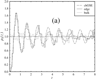
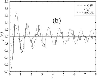
Figure 1: The spectral density at the edge on the scale of the mean level spacing calculated from the lattice data and from the chGSE prediction is compared (a) with that in the bulk and (b) with the chGUE prediction.

Figure 1 shows the results for the microscopic spectral density. We found that the agreement with the chGSE is very good for $z<2$, quite impressive in the region $2<z<5$, and getting worse as $z$ increases. It is interesting to discuss what determines the domain of validity of the random-matrix result. The microscopic spectral density at the edge is essentially

$$\rho_{1}(z)=\bar{D}(0)R_{1}(z\bar{D}(0))\;,$$ (25)

where $\bar{D}(0)$ is the local mean level spacing at the edge. In order to obtain agreement between the lattice data and the thermodynamic limit of the microscopic spectral density given by Eq. (8), $z$ has to be small so that $z\bar{D}(0)\ll 1$. This is because by taking the thermodynamic limit in Eq. (7), we treat the argument $\lambda$ of $R_{1}(\lambda)$ as an infinitesimal quantity. Thus, the random-matrix result is valid over a larger range if $\bar{D}(0)$ is small. We have $\bar{D}(0)=1/V\Sigma$, and the actual value of $\bar{D}(0)$ is determined by several factors. It decreases with increasing lattice volume and increasing chiral condensate (everything is in lattice units). The condensate (at fixed lattice volume) depends on the coupling constant and on temperature, and it decreases with both $\beta$ and $T$. Thus, the domain of validity of the random-matrix result is smaller for smaller lattice volume, larger $\beta$, and larger temperature. To quantify these statements would require a systematic study of lattice data at several values of $V$, $\beta$, and $T$ which is beyond the scope of this paper. For the present lattice, we found $\bar{D}(0)\approx 0.0059$. Therefore, agreement with Eq. (8) is restricted to $z\ll 170$. In practice, we observe agreement only for values of $z$ much lower than this upper bound. As we stressed earlier, the volume $V$ has to be identified with $2N$, i.e., with twice the dimension of the matrices in the random-matrix model. Of course, one can also construct $\rho_{1}$ for purely random matrices of finite dimension. In this case, the agreement with Eq. (8) is quite good already for small dimension. In the case of the lattice data, however, the agreement with Eq. (8) is worse for finite $V$ because the lattice Dirac operator has additional non-random components. We thus attribute the disagreement between the lattice data and the prediction of chRMT for $z>5$ to both the validity of the thermodynamic limit and the non-random components of the lattice Dirac operator.

From Fig. 1, we see that the microscopic spectral density has an oscillatory pattern with peaks distributed almost periodically with period $\approx 1$. The position of the $i$-th peak is the most probable value of the $i$-th eigenvalue. The distribution of the eigenvalues at the edge looks somewhat like a picket fence as does the distribution of energy levels of a harmonic oscillator. This is a consequence of the strong repulsion of the eigenvalues with the fixed point $z=0$. The height of a peak decays as $z$ increases and asymptotically tends to $1$. In Fig. 1(a), the spectral density in the bulk (around the midpoint of the spectra) is also plotted for comparison. There are only slight fluctuations around the average value $\rho_{\rm bulk}=1$. We also plot the chGUE result for the microscopic spectral density Verb93 ,

$$\rho_{1}(z)=\frac{\pi^{2}}{2}z[J_{0}^{2}(\pi z)+J_{1}^{2}(\pi z)]$$ (26)

for $N_{f}=\nu=0$, in Fig. 1(b). It can be seen that the peaks of the chGUE are less pronounced and decay faster than those of the chGSE due to its weaker repulsion (Dyson index $\beta=2$ vs $\beta=4$).

In Fig. 2, we plot the averaged number of eigenvalues in the interval $[0,S]$, i.e., the averaged staircase, as a function of $S$ at the edge as well as in the bulk. Again, the agreement with the chGSE, Eq. (21), is good. The short-dashed line represents the homogeneous distribution $\bar{N}=S$ in the bulk. (Note that for the lattice data we consider, the number of eigenvalues is large enough so that for the small range of $S$ shown in Fig. 2, unfolding in the bulk is not actually necessary.) The deviation of the chGSE from the straight line $\bar{N}=S$ at the edge is much larger than that of the chGUE as in the case of the microscopic spectral density.

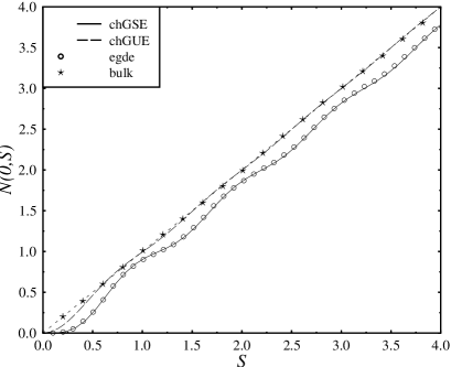
Figure 2: The averaged staircase function at the spectrum edge and in the bulk. The full and the long-dashed line represent the chGSE and the chGUE, respectively. The short-dashed line is $\bar{N}=S$, representing the averaged staircase in the spectrum bulk. The symbols are the data.

Figure 3: The microscopic two-point correlation function $\rho_{2}(z_{1},z_{2})$ and the corresponding microscopic two-point cluster function $\tau_{2}(z_{1},z_{2})$ as functions of $z_{1}$ for fixed $z_{2}$. In (a) and (c), $z_{2}=1.6$, in (b) and (d), $z_{2}=2.6$. The histograms represent lattice data, the dashed lines the chGSE predictions.

We now turn to the two-point correlator. In Fig. 3 we plot the results for $\rho_{2}(z_{1},z_{2})$ and $\tau_{2}(z_{1},z_{2})$ as a function of $z_{1}$ for two fixed values of $z_{2}$, $z_{2}=1.6$ and $z_{2}=2.6$. One can see that the histogram for $\rho_{2}(z_{1},z_{2})$ agrees well with the chGSE prediction, although the agreement is not as good as in Fig. 1 for the one-point function. For $\tau_{2}(z_{1},z_{2})$, the statistics are worse than for $\rho_{2}(z_{1},z_{2})$, except for a small region around $z_{1}=z_{2}$. This is because $\rho_{2}(z_{1},z_{2})$ also includes the one-point functions which are dominant and have better statistics. From the definitions of $\rho_{2}(z_{1},z_{2})$ and $\tau_{2}(z_{1},z_{2})$ we can see that one needs a much larger number of spectra to obtain better statistics. For a given value of $z_{2}$, only those configurations in which there is an eigenvalue in the bin around $z_{2}$ contribute to the two-point function. Even for a value of $z_{2}$ chosen at a peak of $\rho_{1}$ (as in Fig. 3), no more than $1/3$ of the configurations are actually involved in the ensemble average in the construction of $\rho_{2}(z_{1},z_{2})$ and $\tau_{2}(z_{1},z_{2})$ from the data. This is the reason why we only computed $\rho_{2}(z_{1},z_{2})$ and $\tau_{2}(z_{1},z_{2})$ for these specific values of $z_{2}$. For other values, one would have to choose a larger bin size.

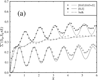
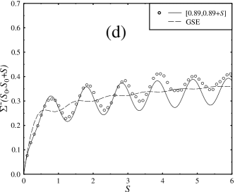
Figure 4: The number variance in an interval $[S_{0},S_{0}+S]$ at the edge with (a) $S_{0}=0$ and 0.63, (b) $S_{0}=0.83$, (c) $S_{0}=0.96$, and (d) $S_{0}=0.89$ as calculated from the lattice data is compared with the corresponding predictions of the chGSE (solid lines) and GSE (dashed lines). For comparison, the number variance in the bulk is computed in (a).

Figure 4 shows our results for the number variance $\Sigma^{2}(S_{0},S_{0}+S)$ at the edge for different values of $S_{0}$ compared with the corresponding chGSE predictions. We also calculated the number variance in the bulk for comparison in Fig. 4(a). No spectral average was performed in the bulk. From this figure, one observes the following points: (i) At the edge, significant systematic deviations from the theoretical prediction occur when $S_{0}+S>4$. The data approach the asymptotic behavior faster than the theoretical curve. Again, this means that the agreement with the thermodynamic limit is restricted to the small region $[0,4\sim 5]$, cf. the discussion after Eq. (25). (ii) For $S\ll 1$, the number variance at the edge increases very slowly, in contrast to the linear relation $\Sigma^{2}=S$ in the bulk. This is simply a manifestation of the suppression of the microscopic spectral density in this region. In fact, from Eq. (22) it can be seen that $\Sigma^{2}$ is dominated by the first term, i.e., by the average staircase function, when $S\ll 1$. The two-point correlations manifest themselves in $\Sigma^{2}(S_{0},S_{0}+S)$ only if $S_{0}+S\geq 1$. (iii) The overall value of $\Sigma^{2}(S_{0},S_{0}+S)$ strongly depends on the value of $S_{0}$. The larger the value of $\rho_{1}(S_{0})$, the larger $\Sigma^{2}(S_{0},S_{0}+S)$. Two extreme cases are shown in Fig. 4(a) where the entire curves of $\Sigma^{2}(S_{0},S_{0}+S)$ are higher resp. lower than the GSE curve. The values $S_{0}=0.63$ and $S_{0}=0$ correspond to the first maximum and minimum of $\rho_{1}$, respectively. Figures 4(b), (c), and (d) show the results for $S_{0}=0.83$, 0.96, and 0.89 with $\rho_{1}(S_{0})<1,>1,$ and $=1$, respectively. (iv) For fixed $S_{0}$, the curves show strong oscillations with peaks appearing when $\rho_{1}(S_{0}+S)$ reaches its maxima. The values of $\Sigma^{2}$ for arbitrary intervals $[S_{1},S_{2}]$ at the edge are distributed around the GSE curve. It is known Meht63 that the number variance reflects the “compressibility” of the eigenvalue “gas”. Therefore, roughly speaking, the compressibility at the edge is on average the same as in the bulk. The case $S_{0}=0$ demands special attention. The very strong suppression shown in Fig. 4(a) is special because the interval starts at the origin which is a fixed point for all spectra so that fluctuations of the eigenvalue number from the left hand side are prohibited. It is always harder to compress this one-dimensional gas on one side than on two sides.

At first glance, one might attribute these features of $\Sigma^{2}$ to the inhomogeneity of the microscopic spectral density. To clarify this point, we will in the next section introduce a microscopic unfolding procedure to remove the oscillations in the microscopic spectral density, and then investigate the effect of the remaining two-point correlations on $\Sigma^{2}$ and $\bar{\Delta}_{3}$.

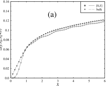
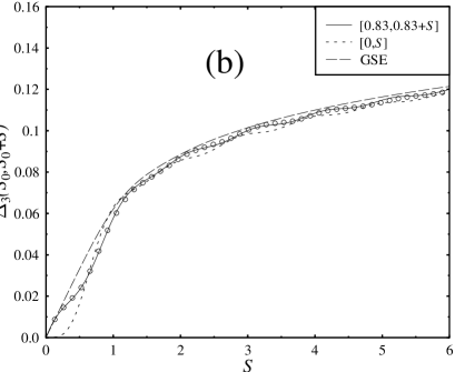
Figure 5: The averaged spectral rigidity at the edge in intervals (a) $[0,S]$ and (b) $[0.83,0.83+S]$ as calculated from the lattice data is compared with chGSE (solid lines) and GSE predictions.

We have also calculated the averaged spectral rigidity both at the edge for various intervals and in the bulk. In Fig. 5 we plot $\bar{\Delta}_{3}(0,S)$ and $\bar{\Delta}_{3}(0.83,0.83+S)$ compared with the corresponding chGSE predictions. We see that the region where the lattice data agree with the prediction of the chGSE is larger than in the case of the number variance, and that the agreement is nearly perfect. In contrast to the case of the number variance, we find that the averaged spectral rigidity at the edge is always smaller than that in the bulk no matter what value of $S_{0}$ is chosen, indicating that the spectrum at the edge is more rigid than in the bulk. Moreover, the difference between the edge and the bulk for the averaged spectral rigidity is small, compared to the significant difference in the case of the number variance. For $S\ll 1$, the behavior of $\bar{\Delta}_{3}(0,S)$ is dominated by the one-point function and lower than the straight line $\bar{\Delta}_{3}=S/15$ in the bulk case. In addition, the curve shows slight convex-concave oscillation with the same period as the oscillations in the number variance and the microscopic spectral density.

4 Microscopic unfolding and two-point correlations

As noted in the previous section, both the number variance and the averaged spectral rigidity at the spectrum edge show oscillations with the same period as the microscopic spectral density. We now wish to clarify whether these oscillations are simply the manifestation of the inhomogeneity of the microscopic spectral density, or are intrinsic in the two-point correlations at the edge. To this end, we first need to separate the variation of the spectral density from the fluctuations on a smaller scale than the microscopic one. This procedure is known as unfolding. We therefore unfold the eigenvalues of all spectra at the edge using the ensemble average of the staircase function,

$${\bar{N}}(z_{i})=\int_{0}^{z_{i}}dz\rho_{1}(z)\;.$$ (27)

Here, $z_{i}$ is the $i$-th eigenvalue measured in terms of the local mean level spacing. Since theoretical results for the staircase function and the microscopic spectral density are available, we can use them directly to unfold the data. The function $\rho_{1}(z)$ is given by Eq. (8).

Figure 6: The number variance calculated from the unfolded lattice data at the edge in an interval (a) $[0,S^{\prime}]$ and in an interval (b) $[0.75,0.75+S^{\prime}]$ corresponding to that in Fig. 4(b).

The microscopic unfolding procedure now works as follows. We introduce a variable transformation from $z$ (which is on the microscopic scale, cf. Eq. (20)) to a new variable $z^{\prime}$,

$$z\to z^{\prime}=\int_{0}^{z}dt\rho_{1}(t)\equiv\omega(z)\;.$$ (28)

We denote the inverse of $\omega(z)$ by $\Omega(z^{\prime})$,

$$z=\Omega(z^{\prime})\;.$$ (29)

In terms of the new variable $z^{\prime}$, the microscopic spectral density becomes

$$\rho^{\prime}_{1}(z^{\prime})=\rho_{1}(z)\frac{dz}{dz^{\prime}}=\rho_{1}\left(\Omega(z^{\prime})\right)\cdot\frac{1}{\rho_{1}\left(\Omega(z^{\prime})\right)}=1$$ (30)

as it should be. The two-point correlation function becomes

$$\rho^{\prime}_{2}(z^{\prime}_{1},z^{\prime}_{2}) = \rho_{2}(z_{1},z_{2})\frac{1}{dz^{\prime}_{1}/dz_{1}\cdot dz^{\prime}_{2}/dz_{2}}$$ (31)

$$= \frac{\rho_{2}(\Omega(z^{\prime}_{1}),\Omega(z^{\prime}_{2}))}{\rho_{1}(\Omega(z^{\prime}_{1}))\rho_{1}(\Omega(z^{\prime}_{2}))}\;,$$

and the two-point cluster function is

$$\tau^{\prime}_{2}(z^{\prime}_{1},z^{\prime}_{2})=1-\rho^{\prime}_{2}(z^{\prime}_{1},z^{\prime}_{2})=\frac{\tau_{2}(\Omega(z^{\prime}_{1}),\Omega(z^{\prime}_{2}))}{\rho_{1}(\Omega(z^{\prime}_{1}))\rho_{1}(\Omega(z^{\prime}_{2}))}\;.$$ (32)

The number variance in an interval $[0,S^{\prime}]$ on the unfolded scale is given by

$$\Sigma^{\prime 2}(0,S^{\prime}) \equiv S^{\prime}-\int_{0}^{S^{\prime}}\int_{0}^{S^{\prime}}dz^{\prime}_{1}dz^{\prime}_{2}\tau^{\prime}_{2}(z^{\prime}_{1},z^{\prime}_{2})$$ (33)

$$=\int_{0}^{\Omega(S^{\prime})}dz\rho_{1}(z)-\int_{0}^{\Omega(S^{\prime})}\int_{0}^{\Omega(S^{\prime})}dz_{1}dz_{2}\tau_{2}(z_{1},z_{2})$$

$$=\Sigma^{2}(0,\Omega(S^{\prime}))\;.$$

But for the spectral rigidity, $\bar{\Delta^{\prime}}_{3}(0,S^{\prime})\neq\bar{\Delta}_{3}(0,\Omega(S^{\prime}))$. Instead,

$$\bar{\Delta^{\prime}}_{3}(0,S^{\prime}) \equiv \frac{S^{\prime}}{15}+\frac{2}{S^{\prime}}\int_{0}^{S^{\prime}}dz^{\prime}_{1}z^{\prime}_{1}\int_{0}^{z^{\prime}_{1}}dz^{\prime}_{2}\tau^{\prime}_{2}(z^{\prime}_{1},z^{\prime}_{2})$$ (34)

$$-\frac{1}{S^{\prime 4}}\int_{0}^{S^{\prime}}\int_{0}^{S^{\prime}}dz^{\prime}_{1}dz^{\prime}_{2}\tau^{\prime}_{2}(z^{\prime}_{1},z^{\prime}_{2})[{S^{\prime}}^{3}(z_{1}^{\prime}+z_{2}^{\prime})$$

$$\phantom{+\frac{1}{S^{\prime 4}}\int_{0}^{S^{\prime}}}-4{S^{\prime}}^{2}z_{1}^{\prime}z_{2}^{\prime}+3S^{\prime}z_{1}^{\prime}z^{\prime}_{2}(z_{1}^{\prime}+z_{2}^{\prime})-3{z_{1}^{\prime}}^{2}{z_{2}^{\prime}}^{2}]$$

$$=\frac{S^{\prime}}{15}+\frac{2}{S^{\prime}}\int_{0}^{\Omega(S^{\prime})}dz_{1}\omega(z_{1})\int_{0}^{z_{1}}dz_{2}\tau_{2}(z_{1},z_{2})$$

$$+\frac{1}{S^{\prime 4}}\int_{0}^{\Omega(S^{\prime})}\int_{0}^{\Omega(S^{\prime})}dz_{1}dz_{2}\tau_{2}(z_{1},z_{2})\{3\omega(z_{1})^{2}\omega(z_{2})^{2}$$

$$-3S^{\prime}\omega(z_{1})\omega(z_{2})[\omega(z_{1})+\omega(z_{2})]$$

$$+4{S^{\prime}}^{2}\omega(z_{1})\omega(z_{2})-{S^{\prime}}^{3}[\omega(z_{1})+\omega(z_{2})]\}\;.$$

Figure 6 shows the number variance at the edge for the unfolded data in the intervals $[0,S^{\prime}]$ and $[0.75,0.75+S^{\prime}]$ corresponding to the intervals $[0,S]$ and $[0.83,0.83+S]$ before unfolding as in Fig. 4, compared with the theoretical prediction of Eq. (33) and its generalization to $[S^{\prime}_{0},S^{\prime}_{0}+S^{\prime}]$. On the unfolded scale, we see that the lattice data agree with the theory in the region $0<S^{\prime}+S^{\prime}_{0}<4$. As expected, for $S^{\prime}\ll 1$ the number variance now returns to the normal case, i.e., to the straight line $\Sigma^{\prime 2}\sim S^{\prime}$. For $S^{\prime}>1$, however, the curves still show oscillations with almost the same amplitude as before unfolding. Also, they still depend strongly on the value of $S^{\prime}_{0}$. The only difference is a small shift along $S^{\prime}$. We therefore come to the conclusion that this kind of oscillation is intrinsic in the two-point correlations, rather than a simple manifestation of the inhomogeneity of the microscopic spectral density. In Fig. 7, we compare the chGSE prediction with those of the chGOE and chGUE under the same conditions, i.e., $N_{f}=0$ and $\nu=0$. One can also see oscillations in the chGOE and chGUE curves, although they are weaker than those of the chGSE.

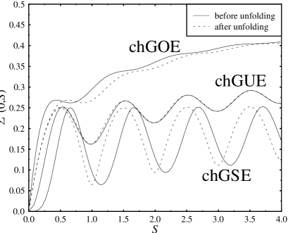
Figure 7: The number variance of the chGOE, chGUE, and chGSE before and after unfolding in an interval $[0,S]$ at the spectrum edge.

We also calculated the averaged spectral rigidity at the edge for the unfolded data and found good agreement with the corresponding chGSE curves, as shown in Fig. 8. We also found that after unfolding the $\bar{\Delta}_{3}$ is larger than that before unfolding and even larger than the GSE result for large $S^{\prime}$. This might imply that the smaller rigidity (compared to the GSE) before unfolding is mainly a manifestation of the oscillations in the one-point function. The picket-fence-like distribution of $\rho_{1}$ makes the spectra very rigid. As before unfolding, a convex-concave oscillation is seen.

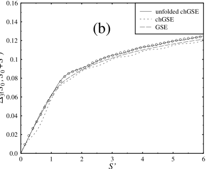
Figure 8: The averaged spectral rigidity calculated from the unfolded lattice data at the edge in an interval (a) $[0,S^{\prime}]$ and in an interval (b) $[0.75,0.75+S^{\prime}]$ corresponding to that in Fig. 5(b).

In Ref. Naga95 , Nagao and Forrester also define an unfolding procedure. Although their definition looks quite different from ours, one can show that they are essentially identical. At first glance, their unfolding seems to remove the global fluctuations of the spectral density defined in terms of the original scale (cf. Eq. (7.7) of Ref. Naga95 ):

$$x\to X=\int_{0}^{x}dx^{\prime}R_{1}(x^{\prime})\;.$$ (35)

However, to have a finite $X$, one has to consider small $x$ so that $x\sim 1/N$ if $N\to\infty$. This corresponds to our rescaling $\lambda\to z=2N\Sigma\lambda/\pi$ before the unfolding of Eq. (27). We must emphasize that because of our microscopic unfolding, the fluctuations on the scale of the mean level spacing ($z\sim 1$) have been changed. Only on the “sub-microscopic” scale ($z\ll 1$) do the fluctuations remain the same as before unfolding. For example, the level-repulsion law on the scale of the mean-level spacing must be the same before and after unfolding. But the “long-range” statistics, like the number variance $\Sigma^{\prime 2}(S^{\prime}_{0},S^{\prime}_{0}+S^{\prime})$, is different from $\Sigma^{2}(S_{0},S_{0}+S)$, as seen in Fig. 6. Nevertheless, our results show that for an ensemble of spectra with a homogeneous spectral density, the number variance can show strong oscillations. Therefore, this kind of oscillation in the number variance can not be attributed to the oscillations in the microscopic spectral density but is inherent in the two-point correlations.

5 On the spacing distribution

We now turn to the short-range statistics. As usual, we define

$$E(L_{0},L_{0}+L)=\mathop{\int\cdots\int}_{{\rm out}}d\lambda_{1}\cdots d\lambda_{N}\rho(\lambda_{1},\ldots,\lambda_{N})\>,$$ (36)

where “out” stands for $[0,L_{0}]$ and $[L_{0}+L,\infty)$. Known as the “hole” probability, $E(L_{0},L_{0}+L)$ is the probability that the interval $[L_{0},L_{0}+L]$ is free of eigenvalues. A related probability density, $F(L_{0},L_{0}+L)$, is defined as

$$F(L_{0},L_{0}+L)=$$ (37)

$$N\mathop{\int\cdots\int}_{{\rm out}}d\lambda_{2}\cdots d\lambda_{N}\rho(L_{0}+L,\lambda_{2},\ldots,\lambda_{N})\;.$$

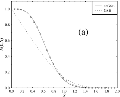
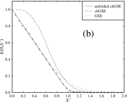
Figure 9: The hole probability $E(0,S)$ (a) before and (b) after microscopic unfolding, compared with the corresponding chGSE predictions. The circles are the lattice data.

$F(L_{0},L_{0}+L)dL$ is the probability that the interval $[L_{0},L_{0}$ $+L]$ is free of eigenvalues and that an eigenvalue is found in $[L_{0}+L,L_{0}+L+dL]$. The nearest-neighbor spacing distribution function is defined as

$$P(L_{0},L_{0}+L)=$$

$$N(N-1)\mathop{\int\cdots\int}_{{\rm out}}d\lambda_{3}\cdots d\lambda_{N}\rho(L_{0},L_{0}+L,\lambda_{3},\ldots,\lambda_{N})$$

so that $P(L_{0},L_{0}+L)dL_{0}dL$ is the probability that two eigenvalues are located in $[L_{0},L_{0}+dL_{0}]$ and $[L_{0}+L,L_{0}+L+dL]$, respectively, and that there is no other eigenvalue between them. Again, we rescale $L\to S=2N\Sigma L/\pi$ to move to the spectrum edge. We then have

$$E(S_{0},S_{0}\!+\!S) = \lim_{N\to\infty}E\left(\frac{\pi S_{0}}{2N\Sigma},\frac{\pi S_{0}}{2N\Sigma}\!+\!\frac{\pi S}{2N\Sigma}\right)\;,$$

$$F(S_{0},S_{0}\!+\!S) = \lim_{N\to\infty}\frac{\pi}{2N\Sigma}F\left(\frac{\pi S_{0}}{2N\Sigma},\frac{\pi S_{0}}{2N\Sigma}\!+\!\frac{\pi S}{2N\Sigma}\right)\;,$$

$$P(S_{0},S_{0}\!+\!S) = \!\!\lim_{N\to\infty}\frac{\pi^{2}}{(2N\Sigma)^{2}}P\left(\frac{\pi S_{0}}{2N\Sigma},\frac{\pi S_{0}}{2N\Sigma}\!+\!\frac{\pi S}{2N\Sigma}\right)\!.$$

For the special case $S_{0}=0$ we obtain, using the results of Ref. Forr93 ,

$$E(0,S) = \frac{\pi}{\sqrt{2}}S^{1/2}\exp(-\pi^{2}S^{2}/2)I_{-1/2}(\pi S)\;,$$ (42)

$$F(0,S) = \frac{\pi^{3}}{\sqrt{2}}S^{3/2}\exp(-\pi^{2}S^{2}/2)I_{3/2}(\pi S)\;,$$ (43)

where $I$ denotes the modified Bessel function. (The two quantities are related by $F(0,S)=-dE(0,S)/dS$.) However,

$$P(0,S)\equiv 0$$ (44)

due to the repulsion between an eigenvalue and the origin inherent in the joint distribution function, Eq. (2). By definition, $F(0,S)$ is the probability density of the smallest eigenvalue.

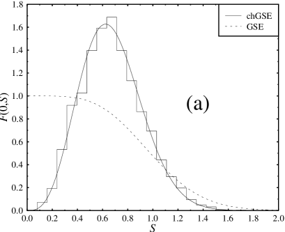
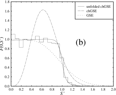
Figure 10: The distribution of the smallest eigenvalue $F(0,S)$ (a) before and (b) after microscopic unfolding, compared with the corresponding chGSE predictions. The histograms represent the lattice data.

Figure 9 shows the results for $E(0,S)$ calculated from the lattice data before and after microscopic unfolding. We again observe nice agreement with the corresponding chGSE predictions. Similar results for $F(0,S)$ are shown in Fig. 10. (Note that $F(0,S)$ plotted in Fig. 10(a) corresponds to the distribution of the smallest eigenvalue obtained in Ref. Berb97a .) From Fig. 9 one can see that, after microscopic unfolding, the shape of $E(0,S)$ becomes closer to that of the usual GSE. The eigenvalues of the Dirac operator always occur in pairs $\pm\lambda_{k}$. Therefore, the function $F(0,S)$ may also be viewed as the nearest-neighbor spacing distribution at the origin if one defines $2S$ as the spacing between the pair $\pm\lambda_{\rm min}$ in units of the mean level spacing. Since the spacing distribution depends on correlators of all order, the nice agreement with the chGSE predictions seen in these two figures provides evidence for the universality of higher-order correlations. For the generic $P(S_{0},S_{0}+S)$ defined in Eq. (5) with $S_{0}\neq 0$ there is, to the best of our knowledge, no theoretical expression available. Of course, it can be constructed from the lattice data. We found that for a generic value of $S_{0}$, the histogram (which is not shown here) is quite different from the usual GSE prediction. It would be interesting to investigate this problem further.

6 Summary

We have studied the spectral statistics of the Dirac spectrum in an SU(2) gauge theory with staggered fermions, restricting ourselves to an $8^{4}$ lattice, with emphasis on the long-range statistics, i.e., the number variance and the spectral rigidity, at the spectrum edge near zero virtuality. Our analysis shows that while the spectra at the edge are more rigid than in the bulk, the fluctuations are suppressed, on average, to the same extent as in the bulk. The strong oscillation in $\Sigma^{2}$ is an edge effect due to the two-point correlations, in the sense that it cannot be removed by microscopic unfolding. On the other hand, the larger rigidity is due to the picket-fence-like behavior of the one-point function, and can be reduced by microscopic unfolding. The excellent agreement between the lattice data and the predictions from chiral random-matrix theory provide direct evidence for the universality of the one- and two-point spectral correlations at the edge. Our study of the spacing distribution demonstrates this universality also for higher-order correlations.

Since our study was only done for one particular lattice size and one particular value of $\beta$, it is in order to discuss the effect of these two parameters on our results. The random-matrix results to which we compare, in particular Eqs. (8) and (14), were derived in the thermodynamic limit. Thus, the agreement between lattice data and chRMT predictions will improve with increasing physical volume $V$, i.e., with increasing lattice size and decreasing $\beta$. We have confirmed this expectation investigating lattice data by Berbenni-Bitsch and Meyer obtained for a number of $\beta$-values in the region $1.8\cdots 2.5$ and lattice sizes between $6^{4}$ and $16^{4}$. It should be emphasized that for any given value of $\beta$ one will eventually find agreement between lattice data and chRMT, provided that the lattice is big enough. Of course, there are practical constraints. Furthermore, chRMT cannot predict a priori how good the agreement will be for a given set of lattice parameters. However, the criterion after Eq. (25) gives an estimate for the quality of the agreement. The mean level spacing at the spectrum edge has to be much smaller than $1/a$, where $a$ is the lattice constant.

After all these demonstrations of universality, one interesting question is the one of practical applications. One possibility is the improvement of extrapolations to the thermodynamic limit, as shown in Ref. Berb97b . Another issue is the extrapolation to the chiral limit in the presence of dynamical fermions. Lattice data for such an investigation are just becoming available, and analytical work on the appropriate random-matrix model is in progress.

- (1) O. Bohigas and M.J. Giannoni, Lec. Not. Phys. 209 (Springer, Heidelberg, 1984).
- (2) E.V. Shuryak and J.J.M. Verbaarschot, Nucl. Phys. A 560, 306 (1993).
- (3) J.J.M. Verbaarschot, Phys. Rev. Lett. 72, 2531 (1994).
- (4) J.J.M. Verbaarschot, hep-th/9710114.
- (5) M.A. Halasz and J.J.M. Verbaarschot, Phys. Rev. Lett. 74, 3920 (1995); M.A. Halasz, T. Kalkreuter, and J.J.M. Verbaarschot, Nucl. Phys. B (Proc. Supp.) 53, 266 (1997).
- (6) T. Wilke, private communication.
- (7) D. Fox and P.B. Kahn, Phys. Rev. 134, B1151 (1964); T. Nagao and M. Wadati, J. Phys. Soc. Jpn. 60, 3298 (1991); 61, 78, 1910 (1992).
- (8) H. Leutwyler and A.V. Smilga, Phys. Rev. D 46, 5607 (1992).
- (9) T. Banks and A. Casher, Nucl. Phys. B 169, 103 (1980).
- (10) J.J.M. Verbaarschot and I. Zahed, Phys. Rev. Lett. 70, 3852 (1993).
- (11) J.J.M. Verbaarschot, Nucl. Phys. B 426, 559 (1994).
- (12) T. Nagao and P.J. Forrester, Nucl. Phys. B 435, 401 (1995).
- (13) J.J.M. Verbaarschot, Nucl. Phys. B 427, 534 (1994).
- (14) S. Chandrasekharan and N. Christ, Nucl. Phys. B (Proc. Suppl.) 47, 527 (1996).
- (15) J.J.M. Verbaarschot, Phys. Lett. B 368, 137 (1996).
- (16) E. Brézin, S. Hikami, and A. Zee, Nucl. Phys. B 464, 411 (1996).
- (17) S. Nishigaki, Phys. Lett. B 387, 139 (1996); G. Akemann, P.H. Damgaard, U. Magnea, and S. Nishigaki, Nucl. Phys. B 487, 721 (1997).
- (18) K. Slevin and T. Nagao, Phys. Rev. Lett. 70, 635 (1993).
- (19) A.D. Jackson, M.K. Şener, and J.J.M. Verbaarschot, Nucl. Phys. B 479, 707 (1996), Nucl. Phys. B 506, 612 (1997); T. Guhr and T. Wettig, Nucl. Phys. B 506, 589 (1997).
- (20) M.E. Berbenni-Bitsch, S. Meyer, A. Schäfer, J.J.M. Verbaarschot, and T. Wettig, hep-lat/9704018, to appear in Phys. Rev. Lett.
- (21) A.D. Jackson and J.J.M. Verbaarschot, Phys. Rev. D 53, 7223 (1996).
- (22) T. Wettig, A. Schäfer, and H.A. Weidenmüller, Phys. Lett. B 367, 28 (1996).
- (23) M.A. Stephanov, Phys. Lett. B 375, 249 (1996).
- (24) M.A. Stephanov, Phys. Rev. Lett. 76, 4472 (1996).
- (25) M.A. Nowak, G. Papp, and I. Zahed, Phys. Lett. B 389, 137, 341 (1996); for a review, see R.A. Janik, M.A. Nowak, G. Papp, and I. Zahed, hep-th/9710103.
- (26) R.A. Janik, M.A. Nowak, and I. Zahed, Phys. Lett. B 392, 155 (1997).
- (27) M.A. Halasz, A.D. Jackson, and J.J.M. Verbaarschot, Phys. Lett. B 395, 293 (1997); Phys. Rev. D 56, 5140 (1997).
- (28) M.A. Halasz, J.C. Osborn, and J.J.M. Verbaarschot, Phys. Rev. D 56, 7059 (1997).
- (29) R.A. Janik, M.A. Nowak, G. Papp, and I. Zahed, Nucl. Phys. B 498, 313 (1997).
- (30) M.E. Berbenni-Bitsch, A.D. Jackson, S. Meyer, A. Schäfer, J.J.M. Verbaarschot, and T. Wettig, hep-lat/9709102.
- (31) M.L. Mehta, Random Matrices, 2nd ed. (Academic Press, San Diego, 1991).
- (32) M.L. Mehta and F.J. Dyson, J. Math. Phys. 4, 713 (1963).
- (33) P.J. Forrester, Nucl. Phys. B 402, 709 (1993).