The Self Energy of Massive Lattice Fermions

Abstract

We address the perturbative renormalization of massive lattice fermions. We derive expressions—valid to all orders in perturbation theory and for all values of the bare fermion mass—for the rest mass, the kinetic mass, and the wave-function renormalization factor. We obtain the fermion’s self energy at the one-loop level with a mass-dependent, $O(a)$ improved action. Numerical results for two interesting special cases, the Wilson and Sheikholeslami-Wohlert actions, are given. The mass dependence of these results smoothly connects the massless and infinite-mass limits, as expected. Combined with Monte Carlo calculations our results can be employed to determine the quark masses in common renormalization schemes.

I Introduction

For some time a goal of lattice QCD has been to determine the masses of the quarks. To be precise, one would like to quote a value of $\bar{m}(\mu)$, the renormalized mass in the $\overline{\rm MS}$ scheme, at momentum scale $\mu$. This is the convention most often used in the phenomenology of the Standard Model and in attempts to treat the Standard Model as the low-energy limit of a more fundamental theory.

In calculations of the hadron spectrum the bare (lattice) mass is a free parameter, which is adjusted to match experiment. The $\overline{\rm MS}$ mass is related to the lattice mass via perturbation theory. This relation is obtained by computing the quark’s pole mass in dimensional regularization and in lattice perturbation theory, and then eliminating the pole mass. For the light quarks the perturbative matching is well established at the one-loop level. The results for the $\overline{\rm MS}$ mass (in the quenched approximation) form a consistent picture, at least when power-law lattice-spacing effects (from the underlying hadron masses) are taken into account [1].

For the charm and bottom quarks lattice artifacts may seem, at first glance, a greater worry, because $m_{q}a$ (the quark mass in lattice units) is not necessarily small. This is, however, not so. Lattice artifacts take the form

$$a\delta E=a^{s_{n}}b_{n}(m_{q}a)\langle\delta H_{n}\rangle$$ (1)

where $\delta H_{n}$ is an operator whose matrix elements are (typically) insensitive or mildly sensitive to the heavy-quark mass, and $b(m_{q}a)$ is a $c$-number function. In the static [2, 3] and nonrelativistic [4, 5] effective theories, which develop an expansion in $1/m_{q}$, Eq. (1) arises by design, and the $b_{n}$ are bounded for large $m_{q}a$. For Wilson-like actions Eq. (1) also holds [6], and the $b_{n}$ are bounded for all $m_{q}a$. To obtain this result, it is essential to avoid expanding around $m_{q}a=0$ or around $m_{q}=\infty$ at every stage of the analysis.

The implication of Ref. [6] for lattice perturbation theory is that the relationship between renormalized and bare quantities is needed for arbitrary $m_{q}a$. This paper examines mass and wave-function renormalization in the class of actions considered in Ref. [6] and gives concrete results at the one-loop level for the Wilson [7] and Sheikholeslami-Wohlert [8] actions. Results are available in the literature for $m_{q}a=0$ [9, 10, 11] and $m_{q}\to\infty$ [3]; as expected [6], the new results presented here smoothly connect the two limits.

The mass dependence of one-loop lattice perturbation theory has been considered before. Results from nonrelativistic theories [12, 13] provide us with cross checks, because (suitable combinations of) their results must agree with ours in the static limit, $m_{q}\to\infty$. At the other extreme, terms of order $m_{q}a$, from expanding our general results around $m_{q}=0$, should recover the results of Sint and Weisz [14].

This paper is organized as follows: Section II discusses the pole in the lattice quark propagator for all $m_{q}a$, to all orders in perturbation theory. The action of Ref. [6], special cases of which are the Wilson and Sheikholeslami-Wohlert actions, is reviewed in Sec. III. The main (all orders) results of Sec. II are expanded to first order in $g_{0}^{2}$ in Sec. IV, and expressions for one-loop Feynman diagrams are presented. Some notation necessary for simplifying numerical evaluation of the one-loop diagrams is given in Sec. V. Section VI presents numerical results for the one-loop contributions to the rest mass, the kinetic mass, and the wave function renormalization factor. (Some of the results have appeared previously [15, 16, 17].) As usual, the dominant contributions come from tadpole diagrams; the results of Sec. VI are improved by “mean-field theory” [18] in Sec. VII. Some technical details are deferred to the Appendices.

The perturbation theory of this paper will be combined with Monte Carlo calculations of the quarkonium and heavy-light spectrum, to determine $\overline{\rm MS}$ masses $\bar{m}_{\text{ch}}$ and $\bar{m}_{\text{b}}$, in forthcoming publications [19].

II Renormalization to All Orders in Perturbation Theory

The objective of this section is to derive relations for mass and wave-function renormalization, for arbitrary values of $m_{q}a$. To do so, we shall assume only properties guaranteed in the lattice theory, and we shall not assume that the self energy is small. By assuming less, we obtain more: our derivation succeeds not only for arbitrary mass, but to all orders in perturbation theory as well.

An outline of our analysis is as follows: We start by anticipating the physical content of the quark propagator, viewed as a function of three-momentum and time. This provides a template from which one can read off the energy, as a function of three-momentum, and the wave-function renormalization factor. We next write down a description of the free propagator and the self energy, as functions of the four-momentum, constrained only by symmetry and periodicity. The description applies to all lattice theories with Wilson’s discretization in time [7]. This includes the Wilson action [7] (of course), the improvements of Ref. [8] and of Ref. [6], and some nonrelativistic actions. Then we Fourier transform the full propagator from four-momentum to time and three-momentum. The result is a sum of terms, one for each pole in the momentum-space propagator. Finally, we focus on the pole corresponding to the one-quark state, and read off the energy and wave-function renormalization factor from the template anticipated at the outset.

In our analysis it is unnecessary to assume that the three-momentum, the mass, or even the self energy itself, is small. Indeed, the notion of a perturbation arises only to separate the inverse full propagator into a free part plus a self energy and to identify a one-quark state in the interacting theory. Thus, our results for the pole are valid not only for all masses but also to all orders in the gauge interaction. (They are not nonperturbative, because quark and gluon states have meaning, in nonabelian gauge theories, only within perturbation theory.) Specializing to small three-momenta (in lattice units), we obtain the three main results of this section: all-orders formulae for the rest mass (Sec. II B), the kinetic mass (Sec. II C), and the wave-function renormalization factor (Sec. II D). In subsequent sections, we specialize further, first to expressions for the one-loop self energy for the action given in Ref. [6], and later to numerical results for the Wilson and Sheikholeslami-Wohlert actions.

A The Quark Pole

Because of confinement, the true states of QCD are hadrons, not quarks and gluons. In perturbation theory, however, one may pretend that quark and gluon states exist. Although the aim of this section is to relate the bare mass of lattice QCD to the perturbative pole mass, one should always view the pole mass as an intermediate step. In a final application, the pole mass should be related to another regulator mass, such as the $\overline{\rm MS}$ mass, or to a genuine (hadronic) observable.

Mindful of the preceding caution, we proceed as if quarks and gluons are physical states. The starting point is the quark two-point correlation function

$$\langle\psi(t,\mathchoice{{\hbox{\boldmath$\displaystyle p$}}}{{\hbox{\boldmath$\textstyle p$}}}{{\hbox{\boldmath$\scriptstyle p$}}}{{\hbox{\boldmath$\scriptscriptstyle p$}}}^{\prime})\bar{\psi}(0,\mathchoice{{\hbox{\boldmath$\displaystyle p$}}}{{\hbox{\boldmath$\textstyle p$}}}{{\hbox{\boldmath$\scriptstyle p$}}}{{\hbox{\boldmath$\scriptscriptstyle p$}}})\rangle=(2\pi)^{3}\delta(\mathchoice{{\hbox{\boldmath$\displaystyle p$}}}{{\hbox{\boldmath$\textstyle p$}}}{{\hbox{\boldmath$\scriptstyle p$}}}{{\hbox{\boldmath$\scriptscriptstyle p$}}}-\mathchoice{{\hbox{\boldmath$\displaystyle p$}}}{{\hbox{\boldmath$\textstyle p$}}}{{\hbox{\boldmath$\scriptstyle p$}}}{{\hbox{\boldmath$\scriptscriptstyle p$}}}^{\prime})G(t,\mathchoice{{\hbox{\boldmath$\displaystyle p$}}}{{\hbox{\boldmath$\textstyle p$}}}{{\hbox{\boldmath$\scriptstyle p$}}}{{\hbox{\boldmath$\scriptscriptstyle p$}}}),$$ (2)

which defines $G(t,\mathchoice{{\hbox{\boldmath$\displaystyle p$}}}{{\hbox{\boldmath$\textstyle p$}}}{{\hbox{\boldmath$\scriptstyle p$}}}{{\hbox{\boldmath$\scriptscriptstyle p$}}})$. The fields are those appearing in the functional integral: they are bare fields, in a fixed gauge chosen so that $G$ does not vanish trivially. The field $\bar{\psi}(0,\mathchoice{{\hbox{\boldmath$\displaystyle p$}}}{{\hbox{\boldmath$\textstyle p$}}}{{\hbox{\boldmath$\scriptstyle p$}}}{{\hbox{\boldmath$\scriptscriptstyle p$}}})$ can create from the vacuum not just the one-quark state, but also states with extra gluons or extra $q\bar{q}$ pairs. One thus anticipates

$$G(t,\mathchoice{{\hbox{\boldmath$\displaystyle p$}}}{{\hbox{\boldmath$\textstyle p$}}}{{\hbox{\boldmath$\scriptstyle p$}}}{{\hbox{\boldmath$\scriptscriptstyle p$}}})={\cal Z}_{2}(\mathchoice{{\hbox{\boldmath$\displaystyle p$}}}{{\hbox{\boldmath$\textstyle p$}}}{{\hbox{\boldmath$\scriptstyle p$}}}{{\hbox{\boldmath$\scriptscriptstyle p$}}})e^{-E(\mathchoice{{\hbox{\boldmath$\displaystyle p$}}}{{\hbox{\boldmath$\textstyle p$}}}{{\hbox{\boldmath$\scriptstyle p$}}}{{\hbox{\boldmath$\scriptscriptstyle p$}}})|t|}Q(\mathchoice{{\hbox{\boldmath$\displaystyle p$}}}{{\hbox{\boldmath$\textstyle p$}}}{{\hbox{\boldmath$\scriptstyle p$}}}{{\hbox{\boldmath$\scriptscriptstyle p$}}})+\int\frac{d^{3}k}{(2\pi)^{3}}{\cal Z}_{qg}(\mathchoice{{\hbox{\boldmath$\displaystyle p$}}}{{\hbox{\boldmath$\textstyle p$}}}{{\hbox{\boldmath$\scriptstyle p$}}}{{\hbox{\boldmath$\scriptscriptstyle p$}}},\mathchoice{{\hbox{\boldmath$\displaystyle k$}}}{{\hbox{\boldmath$\textstyle k$}}}{{\hbox{\boldmath$\scriptstyle k$}}}{{\hbox{\boldmath$\scriptscriptstyle k$}}})e^{-E_{qg}(\mathchoice{{\hbox{\boldmath$\displaystyle p$}}}{{\hbox{\boldmath$\textstyle p$}}}{{\hbox{\boldmath$\scriptstyle p$}}}{{\hbox{\boldmath$\scriptscriptstyle p$}}},\mathchoice{{\hbox{\boldmath$\displaystyle k$}}}{{\hbox{\boldmath$\textstyle k$}}}{{\hbox{\boldmath$\scriptstyle k$}}}{{\hbox{\boldmath$\scriptscriptstyle k$}}})|t|}+\cdots,$$ (3)

where $E(\mathchoice{{\hbox{\boldmath$\displaystyle p$}}}{{\hbox{\boldmath$\textstyle p$}}}{{\hbox{\boldmath$\scriptstyle p$}}}{{\hbox{\boldmath$\scriptscriptstyle p$}}})$ denotes the energy of the one-quark state with momentum $\textstyle p$, and $E_{qg}$ the energy of states with a quark and a gluon. (The quark-gluon states and the multi-particle states denoted by the ellipsis will not concern us further.) If the $\gamma$ matrix $Q(\mathchoice{{\hbox{\boldmath$\displaystyle p$}}}{{\hbox{\boldmath$\textstyle p$}}}{{\hbox{\boldmath$\scriptstyle p$}}}{{\hbox{\boldmath$\scriptscriptstyle p$}}})$ is normalized according to the condition given in Sec. II D, then the residue ${\cal Z}_{2}(\mathchoice{{\hbox{\boldmath$\displaystyle p$}}}{{\hbox{\boldmath$\textstyle p$}}}{{\hbox{\boldmath$\scriptstyle p$}}}{{\hbox{\boldmath$\scriptscriptstyle p$}}})$ is the square of the amplitude for the bare field to create a physical one-quark state.

With a Euclidean invariant cutoff the energy would satisfy $E(\mathchoice{{\hbox{\boldmath$\displaystyle p$}}}{{\hbox{\boldmath$\textstyle p$}}}{{\hbox{\boldmath$\scriptstyle p$}}}{{\hbox{\boldmath$\scriptscriptstyle p$}}})=\sqrt{\mathchoice{{\hbox{\boldmath$\displaystyle p$}}}{{\hbox{\boldmath$\textstyle p$}}}{{\hbox{\boldmath$\scriptstyle p$}}}{{\hbox{\boldmath$\scriptscriptstyle p$}}}^{2}+m^{2}}$, where $m$ is the quark’s “pole” mass. With a lattice cutoff, on the other hand, the mass shell is distorted. To describe the distorted pole position in a systematic way, one can define a rest mass

$$M_{1}=E(\mathchoice{{\hbox{\boldmath$\displaystyle 0$}}}{{\hbox{\boldmath$\textstyle 0$}}}{{\hbox{\boldmath$\scriptstyle 0$}}}{{\hbox{\boldmath$\scriptscriptstyle 0$}}}),$$ (4)

a kinetic mass

$$M_{2}=\left(\frac{\partial^{2}E}{\partial p_{1}^{2}}\right)^{-1}_{\mathchoice{{\hbox{\boldmath$\displaystyle p$}}}{{\hbox{\boldmath$\textstyle p$}}}{{\hbox{\boldmath$\scriptstyle p$}}}{{\hbox{\boldmath$\scriptscriptstyle p$}}}=\mathchoice{{\hbox{\boldmath$\displaystyle 0$}}}{{\hbox{\boldmath$\textstyle 0$}}}{{\hbox{\boldmath$\scriptstyle 0$}}}{{\hbox{\boldmath$\scriptscriptstyle 0$}}}},$$ (5)

and so on. In general $M_{1}\neq M_{2}$, though as $a\to 0$ one should find $M_{2}\to M_{1}$. Alternatively, at nonzero lattice spacing one can impose $M_{2}=M_{1}$ as a requirement on an improved action [6].

Similarly, with a Euclidean invariant cutoff the residue ${\cal Z}_{2}(p)$ would be a function of $p^{2}$ only, evaluated on shell at $p^{2}=-m^{2}$. It is thus a constant independent of $\textstyle p$; it is the wave-function renormalization factor $Z_{2}$. With a lattice cutoff, however, the $\textstyle p$ dependence does not drop out of the residue, even on shell. A reasonable definition of the wave-function renormalization factor is the residue at vanishing three-momentum

$$Z_{2}={\cal Z}_{2}(\mathchoice{{\hbox{\boldmath$\displaystyle 0$}}}{{\hbox{\boldmath$\textstyle 0$}}}{{\hbox{\boldmath$\scriptstyle 0$}}}{{\hbox{\boldmath$\scriptscriptstyle 0$}}}).$$ (6)

Then $Z_{2}^{-1/2}\bar{\psi}$ creates the one-quark state with conventional (unit) normalization, at least for momenta much lower than the ultraviolet cutoff.

To obtain perturbative expressions for $E(\mathchoice{{\hbox{\boldmath$\displaystyle p$}}}{{\hbox{\boldmath$\textstyle p$}}}{{\hbox{\boldmath$\scriptstyle p$}}}{{\hbox{\boldmath$\scriptscriptstyle p$}}})$ and ${\cal Z}_{2}(\mathchoice{{\hbox{\boldmath$\displaystyle p$}}}{{\hbox{\boldmath$\textstyle p$}}}{{\hbox{\boldmath$\scriptstyle p$}}}{{\hbox{\boldmath$\scriptscriptstyle p$}}})$, one starts in momentum space. The inverse full propagator is written

$$G^{-1}(p)=G_{0}^{-1}(p)-\Sigma(p),$$ (7)

where the self energy $\Sigma(p)$ is the sum of all one-particle irreducible graphs. Given $G_{0}$ and $\Sigma$ one obtains the Fourier transform

$$G(t,\mathchoice{{\hbox{\boldmath$\displaystyle p$}}}{{\hbox{\boldmath$\textstyle p$}}}{{\hbox{\boldmath$\scriptstyle p$}}}{{\hbox{\boldmath$\scriptscriptstyle p$}}})=\int_{-\pi/a}^{\pi/a}\frac{dp_{0}}{2\pi}\,e^{ip_{0}t}G(p_{0},\mathchoice{{\hbox{\boldmath$\displaystyle p$}}}{{\hbox{\boldmath$\textstyle p$}}}{{\hbox{\boldmath$\scriptstyle p$}}}{{\hbox{\boldmath$\scriptscriptstyle p$}}})$$ (8)

and compares with Eq. (3) to obtain $E(\mathchoice{{\hbox{\boldmath$\displaystyle p$}}}{{\hbox{\boldmath$\textstyle p$}}}{{\hbox{\boldmath$\scriptstyle p$}}}{{\hbox{\boldmath$\scriptscriptstyle p$}}})$, ${\cal Z}_{2}(\mathchoice{{\hbox{\boldmath$\displaystyle p$}}}{{\hbox{\boldmath$\textstyle p$}}}{{\hbox{\boldmath$\scriptstyle p$}}}{{\hbox{\boldmath$\scriptscriptstyle p$}}})$, and $Q(\mathchoice{{\hbox{\boldmath$\displaystyle p$}}}{{\hbox{\boldmath$\textstyle p$}}}{{\hbox{\boldmath$\scriptstyle p$}}}{{\hbox{\boldmath$\scriptscriptstyle p$}}})$.

We now introduce suitably general expressions for the propagator. For the lattice theories under consideration one can write the inverse free propagator as

$$aG_{0}^{-1}(p)=i\kern 0.50003pt/\kern-6.99997ptK(p)+L(p),$$ (9)

where

$$K_{0}(p_{0},\mathchoice{{\hbox{\boldmath$\displaystyle p$}}}{{\hbox{\boldmath$\textstyle p$}}}{{\hbox{\boldmath$\scriptstyle p$}}}{{\hbox{\boldmath$\scriptscriptstyle p$}}}) = \sin(p_{0}a),$$ (10)

$$\mathchoice{{\hbox{\boldmath$\displaystyle K$}}}{{\hbox{\boldmath$\textstyle K$}}}{{\hbox{\boldmath$\scriptstyle K$}}}{{\hbox{\boldmath$\scriptscriptstyle K$}}}(p_{0},\mathchoice{{\hbox{\boldmath$\displaystyle p$}}}{{\hbox{\boldmath$\textstyle p$}}}{{\hbox{\boldmath$\scriptstyle p$}}}{{\hbox{\boldmath$\scriptscriptstyle p$}}}) = \mathchoice{{\hbox{\boldmath$\displaystyle K$}}}{{\hbox{\boldmath$\textstyle K$}}}{{\hbox{\boldmath$\scriptstyle K$}}}{{\hbox{\boldmath$\scriptscriptstyle K$}}}(\mathchoice{{\hbox{\boldmath$\displaystyle p$}}}{{\hbox{\boldmath$\textstyle p$}}}{{\hbox{\boldmath$\scriptstyle p$}}}{{\hbox{\boldmath$\scriptscriptstyle p$}}}),$$ (11)

$$L(p_{0},\mathchoice{{\hbox{\boldmath$\displaystyle p$}}}{{\hbox{\boldmath$\textstyle p$}}}{{\hbox{\boldmath$\scriptstyle p$}}}{{\hbox{\boldmath$\scriptscriptstyle p$}}}) = \mu(\mathchoice{{\hbox{\boldmath$\displaystyle p$}}}{{\hbox{\boldmath$\textstyle p$}}}{{\hbox{\boldmath$\scriptstyle p$}}}{{\hbox{\boldmath$\scriptscriptstyle p$}}})-\cos(p_{0}a).$$ (12)

The exhibited $p_{0}$ dependence corresponds to Wilson’s discretization, but the functions $\mathchoice{{\hbox{\boldmath$\displaystyle K$}}}{{\hbox{\boldmath$\textstyle K$}}}{{\hbox{\boldmath$\scriptstyle K$}}}{{\hbox{\boldmath$\scriptscriptstyle K$}}}(\mathchoice{{\hbox{\boldmath$\displaystyle p$}}}{{\hbox{\boldmath$\textstyle p$}}}{{\hbox{\boldmath$\scriptstyle p$}}}{{\hbox{\boldmath$\scriptscriptstyle p$}}})$ and $\mu(\mathchoice{{\hbox{\boldmath$\displaystyle p$}}}{{\hbox{\boldmath$\textstyle p$}}}{{\hbox{\boldmath$\scriptstyle p$}}}{{\hbox{\boldmath$\scriptscriptstyle p$}}})$ depend on the action. We assume the action conserves parity, hence $\mathchoice{{\hbox{\boldmath$\displaystyle K$}}}{{\hbox{\boldmath$\textstyle K$}}}{{\hbox{\boldmath$\scriptstyle K$}}}{{\hbox{\boldmath$\scriptscriptstyle K$}}}(\mathchoice{{\hbox{\boldmath$\displaystyle p$}}}{{\hbox{\boldmath$\textstyle p$}}}{{\hbox{\boldmath$\scriptstyle p$}}}{{\hbox{\boldmath$\scriptscriptstyle p$}}})$ is an odd function of $\textstyle p$, and $\mu(\mathchoice{{\hbox{\boldmath$\displaystyle p$}}}{{\hbox{\boldmath$\textstyle p$}}}{{\hbox{\boldmath$\scriptstyle p$}}}{{\hbox{\boldmath$\scriptscriptstyle p$}}})$ even. The couplings are not explicit here, but reappear below as coefficients in the Taylor expansion of $\textstyle K$ and $\mu$ around $\mathchoice{{\hbox{\boldmath$\displaystyle p$}}}{{\hbox{\boldmath$\textstyle p$}}}{{\hbox{\boldmath$\scriptstyle p$}}}{{\hbox{\boldmath$\scriptscriptstyle p$}}}=\mathchoice{{\hbox{\boldmath$\displaystyle 0$}}}{{\hbox{\boldmath$\textstyle 0$}}}{{\hbox{\boldmath$\scriptstyle 0$}}}{{\hbox{\boldmath$\scriptscriptstyle 0$}}}$. For example, $\mu(\mathchoice{{\hbox{\boldmath$\displaystyle 0$}}}{{\hbox{\boldmath$\textstyle 0$}}}{{\hbox{\boldmath$\scriptstyle 0$}}}{{\hbox{\boldmath$\scriptscriptstyle 0$}}})=1+m_{0}a$, where $m_{0}a$ is the bare mass.

We decompose the self energy into $\gamma$ matrices similarly to Eq. (9)

$$a\Sigma(p)=i\sum_{\rho}\gamma_{\rho}A_{\rho}(p)\sin(p_{\rho}a)+C(p).$$ (13)

With a Euclidean invariant cutoff $A_{\rho}=A$ would be a single function for all $\rho$, and $A$ and $C$ would depend on $p^{2}$ only. With a lattice cutoff, however, they are constrained only by (hyper)cubic symmetry. For example, symmetry under parity implies that $A_{\rho}(p_{0},\mathchoice{{\hbox{\boldmath$\displaystyle p$}}}{{\hbox{\boldmath$\textstyle p$}}}{{\hbox{\boldmath$\scriptstyle p$}}}{{\hbox{\boldmath$\scriptscriptstyle p$}}})$ and $C(p_{0},\mathchoice{{\hbox{\boldmath$\displaystyle p$}}}{{\hbox{\boldmath$\textstyle p$}}}{{\hbox{\boldmath$\scriptstyle p$}}}{{\hbox{\boldmath$\scriptscriptstyle p$}}})$ are even functions of $p_{0}$ and $\textstyle p$; symmetry under cubic rotations implies that $A_{1}(0,p,0,0)=A_{2}(0,0,p,0)$; etc. Furthermore, $A_{\rho}$ and $C$ are periodic functions of $p_{0}$, with period $2\pi/a$. Below we make no assumptions about the self energy, except for these symmetry and periodicity properties.

Substituting Eqs. (9) and (13) into Eq. (8), and adopting lattice units ($a=1$), one finds

$$G(t,\mathchoice{{\hbox{\boldmath$\displaystyle p$}}}{{\hbox{\boldmath$\textstyle p$}}}{{\hbox{\boldmath$\scriptstyle p$}}}{{\hbox{\boldmath$\scriptscriptstyle p$}}})=\int_{-\pi}^{\pi}\frac{dp_{0}}{2\pi}\frac{e^{ip_{0}t}N(p_{0},\mathchoice{{\hbox{\boldmath$\displaystyle p$}}}{{\hbox{\boldmath$\textstyle p$}}}{{\hbox{\boldmath$\scriptstyle p$}}}{{\hbox{\boldmath$\scriptscriptstyle p$}}})}{2\nu(p_{0},\mathchoice{{\hbox{\boldmath$\displaystyle p$}}}{{\hbox{\boldmath$\textstyle p$}}}{{\hbox{\boldmath$\scriptstyle p$}}}{{\hbox{\boldmath$\scriptscriptstyle p$}}})[\cosh{\cal E}(p_{0},\mathchoice{{\hbox{\boldmath$\displaystyle p$}}}{{\hbox{\boldmath$\textstyle p$}}}{{\hbox{\boldmath$\scriptstyle p$}}}{{\hbox{\boldmath$\scriptscriptstyle p$}}})-\cos p_{0}]},$$ (14)

where $\nu(p_{0},\mathchoice{{\hbox{\boldmath$\displaystyle p$}}}{{\hbox{\boldmath$\textstyle p$}}}{{\hbox{\boldmath$\scriptstyle p$}}}{{\hbox{\boldmath$\scriptscriptstyle p$}}})=\mu(\mathchoice{{\hbox{\boldmath$\displaystyle p$}}}{{\hbox{\boldmath$\textstyle p$}}}{{\hbox{\boldmath$\scriptstyle p$}}}{{\hbox{\boldmath$\scriptscriptstyle p$}}})-C(p_{0},\mathchoice{{\hbox{\boldmath$\displaystyle p$}}}{{\hbox{\boldmath$\textstyle p$}}}{{\hbox{\boldmath$\scriptstyle p$}}}{{\hbox{\boldmath$\scriptscriptstyle p$}}})$,

$$N(p_{0},\mathchoice{{\hbox{\boldmath$\displaystyle p$}}}{{\hbox{\boldmath$\textstyle p$}}}{{\hbox{\boldmath$\scriptstyle p$}}}{{\hbox{\boldmath$\scriptscriptstyle p$}}})=i\gamma_{0}\sin p_{0}[1-A_{0}(p_{0},\mathchoice{{\hbox{\boldmath$\displaystyle p$}}}{{\hbox{\boldmath$\textstyle p$}}}{{\hbox{\boldmath$\scriptstyle p$}}}{{\hbox{\boldmath$\scriptscriptstyle p$}}})]+i\sum_{i}\gamma_{i}[K_{i}-\sin p_{i}A_{i}(p_{0},\mathchoice{{\hbox{\boldmath$\displaystyle p$}}}{{\hbox{\boldmath$\textstyle p$}}}{{\hbox{\boldmath$\scriptstyle p$}}}{{\hbox{\boldmath$\scriptscriptstyle p$}}})]-[\nu(p_{0},\mathchoice{{\hbox{\boldmath$\displaystyle p$}}}{{\hbox{\boldmath$\textstyle p$}}}{{\hbox{\boldmath$\scriptstyle p$}}}{{\hbox{\boldmath$\scriptscriptstyle p$}}})-\cos p_{0}],$$ (15)

and

$$2\nu\cosh{\cal E}(p_{0},\mathchoice{{\hbox{\boldmath$\displaystyle p$}}}{{\hbox{\boldmath$\textstyle p$}}}{{\hbox{\boldmath$\scriptstyle p$}}}{{\hbox{\boldmath$\scriptscriptstyle p$}}}) = 1+\nu^{2}+\sum_{i}[K_{i}-A_{i}(p_{0},\mathchoice{{\hbox{\boldmath$\displaystyle p$}}}{{\hbox{\boldmath$\textstyle p$}}}{{\hbox{\boldmath$\scriptstyle p$}}}{{\hbox{\boldmath$\scriptscriptstyle p$}}})\sin p_{i}]^{2}$$ (16)

$$- \sin^{2}p_{0}\{1-[1-A_{0}(p_{0},\mathchoice{{\hbox{\boldmath$\displaystyle p$}}}{{\hbox{\boldmath$\textstyle p$}}}{{\hbox{\boldmath$\scriptstyle p$}}}{{\hbox{\boldmath$\scriptscriptstyle p$}}})]^{2}\}.$$ (17)

For $t\neq 0$ one can integrate over $p_{0}$ by changing variables to $z=e^{ip_{0}\mathop{\rm sgn}t}$; then one has contour integration around the unit circle, and the integral is obtained through the residue theorem.

The integrand has a pole at $z=e^{-E}$, whenever $E$ solves the implicit equation

$$\cosh E=\cosh{\cal E}(iE,\mathchoice{{\hbox{\boldmath$\displaystyle p$}}}{{\hbox{\boldmath$\textstyle p$}}}{{\hbox{\boldmath$\scriptstyle p$}}}{{\hbox{\boldmath$\scriptscriptstyle p$}}}).$$ (18)

No more compact, general expression for $E$ exists but to set $p_{0}=iE$ in Eq. (17). (At fixed order in perturbation theory one solves Eqs. (18) and (17) iteratively.) Solutions of Eq. (18) are parametrized by the three-momentum $\textstyle p$ and will be denoted $E(\mathchoice{{\hbox{\boldmath$\displaystyle p$}}}{{\hbox{\boldmath$\textstyle p$}}}{{\hbox{\boldmath$\scriptstyle p$}}}{{\hbox{\boldmath$\scriptscriptstyle p$}}})$.

In general, the integrand of Eq. (14) has several poles. In perturbation theory one assumes, however, that the self energy is a “small” correction. Then the pole corresponding to the quark state must have a residue that does not vanish as $A_{\rho},\;C\to 0$. Poles corresponding to multi-particle states, on the other hand, must have residues that do vanish in the absence of an interaction.

Given an energy satisfying Eq. (18), one expands $\cosh{\cal E}(-i\ln z,\mathchoice{{\hbox{\boldmath$\displaystyle p$}}}{{\hbox{\boldmath$\textstyle p$}}}{{\hbox{\boldmath$\scriptstyle p$}}}{{\hbox{\boldmath$\scriptscriptstyle p$}}})$ in $z$ around $e^{-E}$

$$\cosh{\cal E}(-i\ln z,\mathchoice{{\hbox{\boldmath$\displaystyle p$}}}{{\hbox{\boldmath$\textstyle p$}}}{{\hbox{\boldmath$\scriptstyle p$}}}{{\hbox{\boldmath$\scriptscriptstyle p$}}}) = \cosh E+z^{-1}(z-e^{-E})\dot{\cal E}(iE,\mathchoice{{\hbox{\boldmath$\displaystyle p$}}}{{\hbox{\boldmath$\textstyle p$}}}{{\hbox{\boldmath$\scriptstyle p$}}}{{\hbox{\boldmath$\scriptscriptstyle p$}}})\sinh E$$ (19)

$$+ O{\mathbf{(}}(z-e^{-E})^{2}{\mathbf{)}},$$ (20)

where

$$\dot{\cal E}=z\frac{d\,}{dz}{\cal E}(-i\ln z,\mathchoice{{\hbox{\boldmath$\displaystyle p$}}}{{\hbox{\boldmath$\textstyle p$}}}{{\hbox{\boldmath$\scriptstyle p$}}}{{\hbox{\boldmath$\scriptscriptstyle p$}}})=\frac{1}{i}\frac{d{\cal E}}{dp_{0}}(p_{0},\mathchoice{{\hbox{\boldmath$\displaystyle p$}}}{{\hbox{\boldmath$\textstyle p$}}}{{\hbox{\boldmath$\scriptstyle p$}}}{{\hbox{\boldmath$\scriptscriptstyle p$}}}).$$ (21)

In applying the residue theorem, the quadratic and higher-order terms drop out, and Eq. (14) becomes

$$G(t,\mathchoice{{\hbox{\boldmath$\displaystyle p$}}}{{\hbox{\boldmath$\textstyle p$}}}{{\hbox{\boldmath$\scriptstyle p$}}}{{\hbox{\boldmath$\scriptscriptstyle p$}}}) = \frac{[1-A_{0}(iE,\mathchoice{{\hbox{\boldmath$\displaystyle p$}}}{{\hbox{\boldmath$\textstyle p$}}}{{\hbox{\boldmath$\scriptstyle p$}}}{{\hbox{\boldmath$\scriptscriptstyle p$}}})][\gamma_{0}\mathop{\rm sgn}t\sinh E-i\mathchoice{{\hbox{\boldmath$\displaystyle\gamma$}}}{{\hbox{\boldmath$\textstyle\gamma$}}}{{\hbox{\boldmath$\scriptstyle\gamma$}}}{{\hbox{\boldmath$\scriptscriptstyle\gamma$}}}\cdot\mathchoice{{\hbox{\boldmath$\displaystyle P$}}}{{\hbox{\boldmath$\textstyle P$}}}{{\hbox{\boldmath$\scriptstyle P$}}}{{\hbox{\boldmath$\scriptscriptstyle P$}}}(\mathchoice{{\hbox{\boldmath$\displaystyle p$}}}{{\hbox{\boldmath$\textstyle p$}}}{{\hbox{\boldmath$\scriptstyle p$}}}{{\hbox{\boldmath$\scriptscriptstyle p$}}})]+\nu(iE,\mathchoice{{\hbox{\boldmath$\displaystyle p$}}}{{\hbox{\boldmath$\textstyle p$}}}{{\hbox{\boldmath$\scriptstyle p$}}}{{\hbox{\boldmath$\scriptscriptstyle p$}}})-\cosh E}{2\nu(iE,\mathchoice{{\hbox{\boldmath$\displaystyle p$}}}{{\hbox{\boldmath$\textstyle p$}}}{{\hbox{\boldmath$\scriptstyle p$}}}{{\hbox{\boldmath$\scriptscriptstyle p$}}})[1+\dot{\cal E}(iE,\mathchoice{{\hbox{\boldmath$\displaystyle p$}}}{{\hbox{\boldmath$\textstyle p$}}}{{\hbox{\boldmath$\scriptstyle p$}}}{{\hbox{\boldmath$\scriptscriptstyle p$}}})]\sinh E}e^{-E|t|}$$ (22)

$$+ \text{other residues},$$ (23)

where, for brevity, $E=E(\mathchoice{{\hbox{\boldmath$\displaystyle p$}}}{{\hbox{\boldmath$\textstyle p$}}}{{\hbox{\boldmath$\scriptstyle p$}}}{{\hbox{\boldmath$\scriptscriptstyle p$}}})$ and

$$P_{i}(\mathchoice{{\hbox{\boldmath$\displaystyle p$}}}{{\hbox{\boldmath$\textstyle p$}}}{{\hbox{\boldmath$\scriptstyle p$}}}{{\hbox{\boldmath$\scriptscriptstyle p$}}})=\frac{K_{i}(\mathchoice{{\hbox{\boldmath$\displaystyle p$}}}{{\hbox{\boldmath$\textstyle p$}}}{{\hbox{\boldmath$\scriptstyle p$}}}{{\hbox{\boldmath$\scriptscriptstyle p$}}})-A_{i}(iE,\mathchoice{{\hbox{\boldmath$\displaystyle p$}}}{{\hbox{\boldmath$\textstyle p$}}}{{\hbox{\boldmath$\scriptstyle p$}}}{{\hbox{\boldmath$\scriptscriptstyle p$}}})\sin p_{i}}{1-A_{0}(iE,\mathchoice{{\hbox{\boldmath$\displaystyle p$}}}{{\hbox{\boldmath$\textstyle p$}}}{{\hbox{\boldmath$\scriptstyle p$}}}{{\hbox{\boldmath$\scriptscriptstyle p$}}})}.$$ (24)

The chosen pole has a residue that remains when the interaction is turned off; thus, it corresponds to the one-quark state. The “other residues” correspond to states other than the one-quark state and are disregarded from now on.

B Rest Mass $M_{1}$

To obtain an expression for the rest mass, one sets $p_{0}=iE(\mathchoice{{\hbox{\boldmath$\displaystyle p$}}}{{\hbox{\boldmath$\textstyle p$}}}{{\hbox{\boldmath$\scriptstyle p$}}}{{\hbox{\boldmath$\scriptscriptstyle p$}}})$ in Eq. (17) and solves for $\nu$. One finds

$$\nu(iE,\mathchoice{{\hbox{\boldmath$\displaystyle p$}}}{{\hbox{\boldmath$\textstyle p$}}}{{\hbox{\boldmath$\scriptstyle p$}}}{{\hbox{\boldmath$\scriptscriptstyle p$}}}) \equiv \mu(\mathchoice{{\hbox{\boldmath$\displaystyle p$}}}{{\hbox{\boldmath$\textstyle p$}}}{{\hbox{\boldmath$\scriptstyle p$}}}{{\hbox{\boldmath$\scriptscriptstyle p$}}})-C(iE,\mathchoice{{\hbox{\boldmath$\displaystyle p$}}}{{\hbox{\boldmath$\textstyle p$}}}{{\hbox{\boldmath$\scriptstyle p$}}}{{\hbox{\boldmath$\scriptscriptstyle p$}}})$$ (25)

$$= \cosh E+(1-A_{0})\sqrt{\sinh^{2}E-\mathchoice{{\hbox{\boldmath$\displaystyle P$}}}{{\hbox{\boldmath$\textstyle P$}}}{{\hbox{\boldmath$\scriptstyle P$}}}{{\hbox{\boldmath$\scriptscriptstyle P$}}}^{2}}.$$ (26)

Setting $\mathchoice{{\hbox{\boldmath$\displaystyle p$}}}{{\hbox{\boldmath$\textstyle p$}}}{{\hbox{\boldmath$\scriptstyle p$}}}{{\hbox{\boldmath$\scriptscriptstyle p$}}}=\mathchoice{{\hbox{\boldmath$\displaystyle 0$}}}{{\hbox{\boldmath$\textstyle 0$}}}{{\hbox{\boldmath$\scriptstyle 0$}}}{{\hbox{\boldmath$\scriptscriptstyle 0$}}}$ in Eq. (26) yields the implicit equation

$$e^{M_{1}}=1+m_{0}+A_{0}(iM_{1},\mathchoice{{\hbox{\boldmath$\displaystyle 0$}}}{{\hbox{\boldmath$\textstyle 0$}}}{{\hbox{\boldmath$\scriptstyle 0$}}}{{\hbox{\boldmath$\scriptscriptstyle 0$}}})\sinh M_{1}-C(iM_{1},\mathchoice{{\hbox{\boldmath$\displaystyle 0$}}}{{\hbox{\boldmath$\textstyle 0$}}}{{\hbox{\boldmath$\scriptstyle 0$}}}{{\hbox{\boldmath$\scriptscriptstyle 0$}}}),$$ (27)

where the parameter

$$m_{0}\equiv\mu(\mathchoice{{\hbox{\boldmath$\displaystyle 0$}}}{{\hbox{\boldmath$\textstyle 0$}}}{{\hbox{\boldmath$\scriptstyle 0$}}}{{\hbox{\boldmath$\scriptscriptstyle 0$}}})-1$$ (28)

is the bare mass. Equation (27), expressing the rest mass to all orders in perturbation theory, is the first main result of this section.

For a massless fermion, the rest mass $M_{1}$ should vanish. The critical bare mass, which induces $M_{1}=0$, is

$$m_{0c}=C(0,\mathchoice{{\hbox{\boldmath$\displaystyle 0$}}}{{\hbox{\boldmath$\textstyle 0$}}}{{\hbox{\boldmath$\scriptstyle 0$}}}{{\hbox{\boldmath$\scriptscriptstyle 0$}}};m_{0c}).$$ (29)

The self energy depends on $m_{0}$ as a parameter, denoted here by the third argument of $C$. Since the lattice actions under consideration do not maintain explicit chiral symmetry, one expects $m_{0c}\neq 0$. When applying Eq. (27) it is useful to take care of this term once and for all and write

$$e^{M_{1}}=1+M_{0}+A_{0}(iM_{1},\mathchoice{{\hbox{\boldmath$\displaystyle 0$}}}{{\hbox{\boldmath$\textstyle 0$}}}{{\hbox{\boldmath$\scriptstyle 0$}}}{{\hbox{\boldmath$\scriptscriptstyle 0$}}})\sinh M_{1}-\bar{C}(iM_{1},\mathchoice{{\hbox{\boldmath$\displaystyle 0$}}}{{\hbox{\boldmath$\textstyle 0$}}}{{\hbox{\boldmath$\scriptstyle 0$}}}{{\hbox{\boldmath$\scriptscriptstyle 0$}}})$$ (30)

where $\bar{C}(iM_{1},\mathchoice{{\hbox{\boldmath$\displaystyle 0$}}}{{\hbox{\boldmath$\textstyle 0$}}}{{\hbox{\boldmath$\scriptstyle 0$}}}{{\hbox{\boldmath$\scriptscriptstyle 0$}}};m_{0})=C(iM_{1},\mathchoice{{\hbox{\boldmath$\displaystyle 0$}}}{{\hbox{\boldmath$\textstyle 0$}}}{{\hbox{\boldmath$\scriptstyle 0$}}}{{\hbox{\boldmath$\scriptscriptstyle 0$}}};m_{0})-m_{0c}$, and

$$M_{0}\equiv m_{0}-m_{0c}=\frac{1}{2\kappa}-\frac{1}{2\kappa_{c}}.$$ (31)

In practice, one determines $m_{0c}$ (or $\kappa_{c}$) nonperturbatively in Monte Carlo calculations and treats $M_{0}$ (rather than $m_{0}$) independently of $g_{0}^{2}$ in perturbation theory.

C Kinetic Mass $M_{2}$

From its definition [Eq. (5)] the kinetic mass requires two derivatives with respect to $p_{1}$. Because the derivatives are applied to on-shell self-energy functions, the total derivative with respect to $p_{1}$ includes an explicit part and an implicit part through the dependence on $E$,

$$\frac{d~{}}{dp_{1}}=\frac{\partial~{}}{\partial p_{1}}+i\frac{\partial E}{\partial p_{1}}\frac{\partial~{}}{\partial p_{0}}.$$ (32)

Differentiating Eq. (26) twice yields

$$\frac{e^{M_{1}}-A_{0}(iM_{1},\mathchoice{{\hbox{\boldmath$\displaystyle 0$}}}{{\hbox{\boldmath$\textstyle 0$}}}{{\hbox{\boldmath$\scriptstyle 0$}}}{{\hbox{\boldmath$\scriptscriptstyle 0$}}})\cosh M_{1}}{M_{2}}=r_{s}\zeta+D(\mathchoice{{\hbox{\boldmath$\displaystyle 0$}}}{{\hbox{\boldmath$\textstyle 0$}}}{{\hbox{\boldmath$\scriptstyle 0$}}}{{\hbox{\boldmath$\scriptscriptstyle 0$}}})+\frac{[\zeta-A_{1}(iM_{1},\mathchoice{{\hbox{\boldmath$\displaystyle 0$}}}{{\hbox{\boldmath$\textstyle 0$}}}{{\hbox{\boldmath$\scriptstyle 0$}}}{{\hbox{\boldmath$\scriptscriptstyle 0$}}})]^{2}}{[1-A_{0}(iM_{1},\mathchoice{{\hbox{\boldmath$\displaystyle 0$}}}{{\hbox{\boldmath$\textstyle 0$}}}{{\hbox{\boldmath$\scriptstyle 0$}}}{{\hbox{\boldmath$\scriptscriptstyle 0$}}})]\sinh M_{1}},$$ (33)

where

$$D(\mathchoice{{\hbox{\boldmath$\displaystyle p$}}}{{\hbox{\boldmath$\textstyle p$}}}{{\hbox{\boldmath$\scriptstyle p$}}}{{\hbox{\boldmath$\scriptscriptstyle p$}}})=\frac{d^{2}~{}}{dp_{1}^{2}}\left[A_{0}(iE(\mathchoice{{\hbox{\boldmath$\displaystyle p$}}}{{\hbox{\boldmath$\textstyle p$}}}{{\hbox{\boldmath$\scriptstyle p$}}}{{\hbox{\boldmath$\scriptscriptstyle p$}}}),\mathchoice{{\hbox{\boldmath$\displaystyle p$}}}{{\hbox{\boldmath$\textstyle p$}}}{{\hbox{\boldmath$\scriptstyle p$}}}{{\hbox{\boldmath$\scriptscriptstyle p$}}})\sinh M_{1}-C(iE(\mathchoice{{\hbox{\boldmath$\displaystyle p$}}}{{\hbox{\boldmath$\textstyle p$}}}{{\hbox{\boldmath$\scriptstyle p$}}}{{\hbox{\boldmath$\scriptscriptstyle p$}}}),\mathchoice{{\hbox{\boldmath$\displaystyle p$}}}{{\hbox{\boldmath$\textstyle p$}}}{{\hbox{\boldmath$\scriptstyle p$}}}{{\hbox{\boldmath$\scriptscriptstyle p$}}})\right].$$ (34)

The quantities

$$\zeta \equiv K^{\prime}_{1}(\mathchoice{{\hbox{\boldmath$\displaystyle 0$}}}{{\hbox{\boldmath$\textstyle 0$}}}{{\hbox{\boldmath$\scriptstyle 0$}}}{{\hbox{\boldmath$\scriptscriptstyle 0$}}}),$$ (35)

$$r_{s}\zeta \equiv \mu^{\prime\prime}(\mathchoice{{\hbox{\boldmath$\displaystyle 0$}}}{{\hbox{\boldmath$\textstyle 0$}}}{{\hbox{\boldmath$\scriptstyle 0$}}}{{\hbox{\boldmath$\scriptscriptstyle 0$}}}),$$ (36)

with primes denoting differentiation with respect to $p_{1}$, are couplings parametrizing the action. Equation (33), expressing the kinetic mass to all orders in perturbation theory, is the second main result of this section.

Without the interaction that generates the self energy, one can solve Eq. (33) in closed form: $M_{2}^{[0]}=m_{2}(M_{1}^{[0]})$, where

$$m_{2}(m)=\frac{e^{m}\sinh m}{\zeta^{2}+r_{s}\zeta\sinh m}.$$ (37)

This expression suggests defining a kinetic-mass renormalization factor $Z_{M_{2}}$ through

$$Z_{M_{2}}=\frac{M_{2}}{m_{2}(M_{1})},$$ (38)

which captures the radiative corrections to $M_{2}$ not shared by $M_{1}$. In perturbation theory a quark’s kinetic and rest masses are on-shell observables. By definition the ratio $Z_{M_{2}}$ is also an on-shell quantity. It is, therefore, a useful diagnostic of cutoff effects in the continuum limit. Indeed,

$$\lim_{M_{1}a\to 0}Z_{M_{2}}=1$$ (39)

to all orders in perturbation theory.

For $M_{1}a\neq 0$ the rest and kinetic masses are not, as a rule, equal. To construct a mass-dependent improved action, as in Ref. [6], one sets $M_{2}=M_{1}$ in Eq. (33) and solves for a condition on the coupling $\zeta$, parametrized by $r_{s}$. In the following we do not, however, assume that such conditions have been imposed.

D Wave-function Renormalization $Z_{2}$

Comparing Eq. (22) with Eq. (3) one identifies the $\gamma$ matrix function of $\textstyle p$ that multiplies $e^{-E(\mathchoice{{\hbox{\boldmath$\displaystyle p$}}}{{\hbox{\boldmath$\textstyle p$}}}{{\hbox{\boldmath$\scriptstyle p$}}}{{\hbox{\boldmath$\scriptscriptstyle p$}}})|t|}$ as ${\cal Z}_{2}Q$. To fix the normalization of $Q$, first write $Q=\mathop{\rm sgn}t\gamma_{0}Q_{0}-{i\mathchoice{{\hbox{\boldmath$\displaystyle\gamma$}}}{{\hbox{\boldmath$\textstyle\gamma$}}}{{\hbox{\boldmath$\scriptstyle\gamma$}}}{{\hbox{\boldmath$\scriptscriptstyle\gamma$}}}\cdot\mathchoice{{\hbox{\boldmath$\displaystyle Q$}}}{{\hbox{\boldmath$\textstyle Q$}}}{{\hbox{\boldmath$\scriptstyle Q$}}}{{\hbox{\boldmath$\scriptscriptstyle Q$}}}}+R$. (Note that $Q_{0}^{2}-\mathchoice{{\hbox{\boldmath$\displaystyle Q$}}}{{\hbox{\boldmath$\textstyle Q$}}}{{\hbox{\boldmath$\scriptstyle Q$}}}{{\hbox{\boldmath$\scriptscriptstyle Q$}}}^{2}-R^{2}=0$ on shell.) In the canonical normalization $Q_{0}=\frac{1}{2}$. Thus,

$${\cal Z}_{2}(\mathchoice{{\hbox{\boldmath$\displaystyle p$}}}{{\hbox{\boldmath$\textstyle p$}}}{{\hbox{\boldmath$\scriptstyle p$}}}{{\hbox{\boldmath$\scriptscriptstyle p$}}})=\frac{1-A_{0}(iE,\mathchoice{{\hbox{\boldmath$\displaystyle p$}}}{{\hbox{\boldmath$\textstyle p$}}}{{\hbox{\boldmath$\scriptstyle p$}}}{{\hbox{\boldmath$\scriptscriptstyle p$}}})}{\nu(iE,\mathchoice{{\hbox{\boldmath$\displaystyle p$}}}{{\hbox{\boldmath$\textstyle p$}}}{{\hbox{\boldmath$\scriptstyle p$}}}{{\hbox{\boldmath$\scriptscriptstyle p$}}})[1+\dot{\cal E}(iE,\mathchoice{{\hbox{\boldmath$\displaystyle p$}}}{{\hbox{\boldmath$\textstyle p$}}}{{\hbox{\boldmath$\scriptstyle p$}}}{{\hbox{\boldmath$\scriptscriptstyle p$}}})]}.$$ (40)

A more explicit expression may be obtained by using Eqs. (17) and (18) to eliminate $\nu(iE,\mathchoice{{\hbox{\boldmath$\displaystyle p$}}}{{\hbox{\boldmath$\textstyle p$}}}{{\hbox{\boldmath$\scriptstyle p$}}}{{\hbox{\boldmath$\scriptscriptstyle p$}}})$ and $\nu\dot{\cal E}(iE,\mathchoice{{\hbox{\boldmath$\displaystyle p$}}}{{\hbox{\boldmath$\textstyle p$}}}{{\hbox{\boldmath$\scriptstyle p$}}}{{\hbox{\boldmath$\scriptscriptstyle p$}}})$. One finds

$${\cal Z}_{2}(\mathchoice{{\hbox{\boldmath$\displaystyle p$}}}{{\hbox{\boldmath$\textstyle p$}}}{{\hbox{\boldmath$\scriptstyle p$}}}{{\hbox{\boldmath$\scriptscriptstyle p$}}})^{-1} = (1-A_{0})\cosh E+\sqrt{\sinh^{2}E-\mathchoice{{\hbox{\boldmath$\displaystyle P$}}}{{\hbox{\boldmath$\textstyle P$}}}{{\hbox{\boldmath$\scriptstyle P$}}}{{\hbox{\boldmath$\scriptscriptstyle P$}}}^{2}}+\dot{A}_{0}\sinh E$$ (41)

$$- \dot{C}\sqrt{1-\mathchoice{{\hbox{\boldmath$\displaystyle P$}}}{{\hbox{\boldmath$\textstyle P$}}}{{\hbox{\boldmath$\scriptstyle P$}}}{{\hbox{\boldmath$\scriptscriptstyle P$}}}^{2}/\sinh^{2}E}-\sum_{j}\frac{\dot{A}_{j}P_{j}\sin p_{j}}{\sinh E},$$ (42)

with all self-energy functions evaluated at $(iE(\mathchoice{{\hbox{\boldmath$\displaystyle p$}}}{{\hbox{\boldmath$\textstyle p$}}}{{\hbox{\boldmath$\scriptstyle p$}}}{{\hbox{\boldmath$\scriptscriptstyle p$}}}),\mathchoice{{\hbox{\boldmath$\displaystyle p$}}}{{\hbox{\boldmath$\textstyle p$}}}{{\hbox{\boldmath$\scriptstyle p$}}}{{\hbox{\boldmath$\scriptscriptstyle p$}}})$. Setting $\mathchoice{{\hbox{\boldmath$\displaystyle p$}}}{{\hbox{\boldmath$\textstyle p$}}}{{\hbox{\boldmath$\scriptstyle p$}}}{{\hbox{\boldmath$\scriptscriptstyle p$}}}=\mathchoice{{\hbox{\boldmath$\displaystyle 0$}}}{{\hbox{\boldmath$\textstyle 0$}}}{{\hbox{\boldmath$\scriptstyle 0$}}}{{\hbox{\boldmath$\scriptscriptstyle 0$}}}$ to obtain the wave-function renormalization factor, as discussed above, one finds

$$Z_{2}^{-1} = {\cal Z}_{2}(\mathchoice{{\hbox{\boldmath$\displaystyle 0$}}}{{\hbox{\boldmath$\textstyle 0$}}}{{\hbox{\boldmath$\scriptstyle 0$}}}{{\hbox{\boldmath$\scriptscriptstyle 0$}}})^{-1}$$ (43)

$$= e^{M_{1}}-A_{0}\cosh M_{1}+\dot{A}_{0}\sinh M_{1}-\dot{C},$$ (44)

where all self-energy functions are evaluated at $(iM_{1},\mathchoice{{\hbox{\boldmath$\displaystyle 0$}}}{{\hbox{\boldmath$\textstyle 0$}}}{{\hbox{\boldmath$\scriptstyle 0$}}}{{\hbox{\boldmath$\scriptscriptstyle 0$}}})$. Note that every term on the right-hand side of Eq. (44) is of order $e^{M_{1}}$ in the large mass limit, just as at tree level. Equation (44), expressing the wave-function renormalization factor for arbitrary values of $M_{1}a$, to all orders in perturbation theory, is the third, and final, main result of this section.

In most gauges, the wave-function renormalization factor is infrared divergent. The divergence cancels against vertex renormalization factors, when a physical combination, such as the full renormalization of a current, is considered.

III The Lattice Action

We consider the action $S=S_{0}+S_{B}+S_{E}$ of Ref. [6], namely

$$S_{0} = m_{0}a^{4}\sum_{x}\bar{\psi}(x)\psi(x)+\frac{1}{2}a^{4}\sum_{x}\bar{\psi}(x)[(1+\gamma_{0})D_{0}^{-}-(1-\gamma_{0})D_{0}^{+}]\psi(x)$$ (45)

$$+ \zeta a^{4}\sum_{x}\bar{\psi}(x)\mathchoice{{\hbox{\boldmath$\displaystyle\gamma$}}}{{\hbox{\boldmath$\textstyle\gamma$}}}{{\hbox{\boldmath$\scriptstyle\gamma$}}}{{\hbox{\boldmath$\scriptscriptstyle\gamma$}}}\cdot\mathchoice{{\hbox{\boldmath$\displaystyle D$}}}{{\hbox{\boldmath$\textstyle D$}}}{{\hbox{\boldmath$\scriptstyle D$}}}{{\hbox{\boldmath$\scriptscriptstyle D$}}}\psi(x)-\frac{1}{2}r_{s}\zeta a^{5}\sum_{x}\bar{\psi}(x)\triangle^{(3)}\psi(x),$$ (46)

where the covariant difference operators are

$$aD_{0}^{\pm}\psi(x)=\pm[U_{\pm 0}(x)\psi(x\pm a\hat{0})-\psi(x)],$$ (47)

$$aD_{i}\psi(x)=\frac{1}{2}[U_{i}\psi(x+a\hat{\imath})-U_{-i}\psi(x-a\hat{\imath})],$$ (48)

and

$$a^{2}\triangle^{(3)}\psi(x)=\sum_{i}\frac{1}{2}\big{[}U_{i}\psi(x+a\hat{\imath})+U_{-i}\psi(x-a\hat{\imath})-2\psi(x)\big{]}.$$ (49)

The action $S_{0}$ has cutoff artifacts of order $a$, which can be canceled by the interactions

$$S_{B}=-\frac{i}{2}a^{5}c_{B}\zeta\sum_{x}\bar{\psi}(x)\mathchoice{{\hbox{\boldmath$\displaystyle\Sigma$}}}{{\hbox{\boldmath$\textstyle\Sigma$}}}{{\hbox{\boldmath$\scriptstyle\Sigma$}}}{{\hbox{\boldmath$\scriptscriptstyle\Sigma$}}}\cdot\mathchoice{{\hbox{\boldmath$\displaystyle B$}}}{{\hbox{\boldmath$\textstyle B$}}}{{\hbox{\boldmath$\scriptstyle B$}}}{{\hbox{\boldmath$\scriptscriptstyle B$}}}(x)\psi(x),$$ (50)

$$S_{E}=-\frac{1}{2}a^{5}c_{E}\zeta\sum_{x}\bar{\psi}(x)\mathchoice{{\hbox{\boldmath$\displaystyle\alpha$}}}{{\hbox{\boldmath$\textstyle\alpha$}}}{{\hbox{\boldmath$\scriptstyle\alpha$}}}{{\hbox{\boldmath$\scriptscriptstyle\alpha$}}}\cdot\mathchoice{{\hbox{\boldmath$\displaystyle E$}}}{{\hbox{\boldmath$\textstyle E$}}}{{\hbox{\boldmath$\scriptstyle E$}}}{{\hbox{\boldmath$\scriptscriptstyle E$}}}(x)\psi(x),$$ (51)

for appropriate adjustments of $c_{B}$ and $c_{E}$. The chromomagnetic and chromoelectric fields are given in Ref. [6].

Special cases of this action are the Wilson action [7], which sets $r_{s}=\zeta=1$, $c_{B}=c_{E}=0$; and the Sheikholeslami-Wohlert action [8], which sets $r_{s}=\zeta=1$, $c_{B}=c_{E}\equiv c_{\text{SW}}$. But to remove lattice artifacts for arbitrary masses, the couplings $r_{s}$, $\zeta$, $c_{B}$ and $c_{E}$ must be taken to depend on $m_{0}a$ [6]. For the purposes of this paper, however, the additional couplings are taken as free parameters.

We note here the elements of the free propagator introduced in Eq. (11). From Eq. (46) one finds

$$K_{i}(\mathchoice{{\hbox{\boldmath$\displaystyle p$}}}{{\hbox{\boldmath$\textstyle p$}}}{{\hbox{\boldmath$\scriptstyle p$}}}{{\hbox{\boldmath$\scriptscriptstyle p$}}}) = \zeta\sin p_{i}a,$$ (52)

$$\mu(\mathchoice{{\hbox{\boldmath$\displaystyle p$}}}{{\hbox{\boldmath$\textstyle p$}}}{{\hbox{\boldmath$\scriptstyle p$}}}{{\hbox{\boldmath$\scriptscriptstyle p$}}}) = 1+m_{0}a+\frac{1}{2}r_{s}\zeta\hat{\mathchoice{{\hbox{\boldmath$\displaystyle p$}}}{{\hbox{\boldmath$\textstyle p$}}}{{\hbox{\boldmath$\scriptstyle p$}}}{{\hbox{\boldmath$\scriptscriptstyle p$}}}}^{2}a^{2},$$ (53)

where $\hat{p}_{i}=(2/a)\sin\frac{1}{2}p_{i}a$. Thus, the notation for the couplings coincides with that in Eqs. (28), (35), and (36).

As the mass tends to infinity, all actions described by $S_{0}+S_{B}+S_{E}$ lead, up to an unphysical factor, to the same quark propagator—a Wilson line. Perturbative corrections to masses and vertices must respect this universal static limit, and, therefore, they must tend to a universal value. This limiting behavior is a helpful check.

IV The Self Energy to One Loop

The analysis of Sec. II is valid to all orders in perturbation theory. We now develop expansions in $g_{0}^{2}$ for the main results, concentrating on the one-loop approximation. We also present our expressions for the one-loop self energy.

A Perturbative Series

In perturbation theory the self energy is expanded

$$\Sigma(p)=\sum_{l=1}^{\infty}g_{0}^{2l}\Sigma^{[l]}(p),$$ (54)

and similarly for the functions $A_{\rho}$ and $C$. As a consequence, the rest mass has an expansion

$$M_{1}=\sum_{l=0}^{\infty}g_{0}^{2l}M_{1}^{[l]}.$$ (55)

where the tree level $M_{1}^{[0]}=\log(1+M_{0})$. The one-loop coefficient, from Eq. (27), is

$$M_{1}^{[1]}=\left[A_{0}^{[1]}(iM_{1}^{[0]},\mathchoice{{\hbox{\boldmath$\displaystyle 0$}}}{{\hbox{\boldmath$\textstyle 0$}}}{{\hbox{\boldmath$\scriptstyle 0$}}}{{\hbox{\boldmath$\scriptscriptstyle 0$}}})\sinh M_{1}^{[0]}-\bar{C}^{[1]}(iM_{1}^{[0]},\mathchoice{{\hbox{\boldmath$\displaystyle 0$}}}{{\hbox{\boldmath$\textstyle 0$}}}{{\hbox{\boldmath$\scriptstyle 0$}}}{{\hbox{\boldmath$\scriptscriptstyle 0$}}})\right]e^{-M_{1}^{[0]}}.$$ (56)

In the massless limit

$$\frac{M_{1}^{[1]}}{M_{1}^{[0]}}=A_{0}^{[1]}-\left.\frac{\partial C^{[1]}}{\partial m_{0}}\right|_{m_{0}=0},$$ (57)

which is the same result as in massless derivations [9]. In the static limit, $A_{0}$ tends to a constant and $C$ to $e^{M_{1}}$ times a constant. Thus, $M_{1}^{[1]}(\infty)$ is finite. Moreover, it is the same for all actions under consideration.

The kinetic-mass renormalization factor has an expansion

$$Z_{M_{2}}=1+\sum_{l=1}^{\infty}g_{0}^{2l}Z_{M_{2}}^{[l]}$$ (58)

The one-loop coefficient, from Eq. (33), is

$$Z_{M_{2}}^{[1]}=\frac{2\zeta A_{1}^{[1]}(iM_{1}^{[0]},\mathchoice{{\hbox{\boldmath$\displaystyle 0$}}}{{\hbox{\boldmath$\textstyle 0$}}}{{\hbox{\boldmath$\scriptstyle 0$}}}{{\hbox{\boldmath$\scriptscriptstyle 0$}}})-\zeta^{2}A_{0}^{[1]}(iM_{1}^{[0]},\mathchoice{{\hbox{\boldmath$\displaystyle 0$}}}{{\hbox{\boldmath$\textstyle 0$}}}{{\hbox{\boldmath$\scriptstyle 0$}}}{{\hbox{\boldmath$\scriptscriptstyle 0$}}})-D^{[1]}(\mathchoice{{\hbox{\boldmath$\displaystyle 0$}}}{{\hbox{\boldmath$\textstyle 0$}}}{{\hbox{\boldmath$\scriptstyle 0$}}}{{\hbox{\boldmath$\scriptscriptstyle 0$}}})\sinh M_{1}^{[0]}}{\zeta^{2}+r_{s}\zeta\sinh M_{1}^{[0]}}-A_{0}^{[1]}(iM_{1}^{[0]},\mathchoice{{\hbox{\boldmath$\displaystyle 0$}}}{{\hbox{\boldmath$\textstyle 0$}}}{{\hbox{\boldmath$\scriptstyle 0$}}}{{\hbox{\boldmath$\scriptscriptstyle 0$}}})\cosh M_{1}^{[0]}e^{-M_{1}^{[0]}}.$$ (59)

In the massless limit, $Z_{M_{2}}^{[1]}$ vanishes at least as fast as $(Ma)^{2}\ln(Ma)$. In the static limit $Z_{M_{2}}^{[1]}\to-D^{[1]}/(r_{s}\zeta)-\frac{1}{2}A_{0}^{[1]}$, again finite. Moreover, it too is the same for all actions under consideration, and it can be compared to the same combination in nonrelativistic QCD.

At tree level many have noticed that the quark propagator’s residue ${\cal Z}_{2}(\mathchoice{{\hbox{\boldmath$\displaystyle 0$}}}{{\hbox{\boldmath$\textstyle 0$}}}{{\hbox{\boldmath$\scriptstyle 0$}}}{{\hbox{\boldmath$\scriptscriptstyle 0$}}})=e^{-M_{1}}$. This dominant (large) mass dependence persists in individual loop diagrams [6] and, as shown in Eq. (44), to all orders. To isolate the subleading mass dependence of the wave-function renormalization, we develop the expansion as follows:

$$e^{M_{1}}Z_{2}=1+\sum_{l=1}^{\infty}g_{0}^{2l}Z_{2}^{[l]},$$ (60)

with the physical (all-orders) rest mass in the exponent on the left-hand side. We apologize for a notation in which $Z_{2}^{[l]}$ is not the perturbative coefficient of $Z_{2}$, but this way the $Z_{2}^{[l]}$ have only mild mass dependence. The one-loop coefficient, from Eq. (44), is

$$Z_{2}^{[1]}=\left[A_{0}^{[1]}(iM_{1}^{[0]},\mathchoice{{\hbox{\boldmath$\displaystyle 0$}}}{{\hbox{\boldmath$\textstyle 0$}}}{{\hbox{\boldmath$\scriptstyle 0$}}}{{\hbox{\boldmath$\scriptscriptstyle 0$}}})\cosh M_{1}^{[0]}-\dot{A}_{0}^{[1]}(iM_{1}^{[0]},\mathchoice{{\hbox{\boldmath$\displaystyle 0$}}}{{\hbox{\boldmath$\textstyle 0$}}}{{\hbox{\boldmath$\scriptstyle 0$}}}{{\hbox{\boldmath$\scriptscriptstyle 0$}}})\sinh M_{1}^{[0]}+\dot{C}^{[1]}(iM_{1}^{[0]},\mathchoice{{\hbox{\boldmath$\displaystyle 0$}}}{{\hbox{\boldmath$\textstyle 0$}}}{{\hbox{\boldmath$\scriptstyle 0$}}}{{\hbox{\boldmath$\scriptscriptstyle 0$}}})\right]e^{-M_{1}^{[0]}}.$$ (61)

In the massless limit, the right-hand side reduces to the well-known result $A_{0}^{[1]}-M\dot{A}_{0}^{[1]}+\dot{C}^{[1]}$. (As $M\to 0$, $M\dot{A}^{[1]}\to\text{const}$.) In the static limit, each term on the right-hand side of approaches a (universal) value, and thus the sum $Z_{2}^{[1]}$ does too.

B One-Loop Diagrams

It is straightforward to derive Feynman rules for $S_{0}+S_{B}+S_{E}$. They are listed in Appendix A. To one loop the self energy is given by the Feynman diagrams in Fig. 1.

FIG. 1.: Feynman diagrams for the one-loop self-energy: (a) rainbow, (b) tadpole.

We use the Wilson gauge action [20]. The rainbow diagram, Fig. 1a, represents the contribution

$$\Sigma^{[1]}_{\text{(a)}}(p)=C_{F}\int\frac{d^{4}k}{(2\pi)^{4}}\frac{F(p,k)}{\hat{k}^{2}[K^{2}(p+k)+L^{2}(p+k)]},$$ (62)

with $K_{\rho}$ and $L$ specified by Eqs. (11), (52), and (53). The numerator $F(p,k)$, which follows from $\gamma$-matrix algebra, is given in Appendix B. The color factor $C_{F}=(N_{c}^{2}-1)/(2N_{c})$ [$=4/3$ for SU(3)]. The tadpole diagram, Fig. 1b, represents a much simpler contribution; in Feynman gauge

$$\Sigma^{[1]}_{\text{(b)}}(p)=\frac{1}{2}C_{F}[i\gamma_{0}\sin p_{0}+i\zeta\mathchoice{{\hbox{\boldmath$\displaystyle\gamma$}}}{{\hbox{\boldmath$\textstyle\gamma$}}}{{\hbox{\boldmath$\scriptstyle\gamma$}}}{{\hbox{\boldmath$\scriptscriptstyle\gamma$}}}\cdot\sin\mathchoice{{\hbox{\boldmath$\displaystyle p$}}}{{\hbox{\boldmath$\textstyle p$}}}{{\hbox{\boldmath$\scriptstyle p$}}}{{\hbox{\boldmath$\scriptscriptstyle p$}}}-\cos p_{0}-r_{s}\zeta\sum_{i}\cos p_{i}]\int\frac{d^{4}k}{(2\pi)^{4}}\frac{1}{\hat{k}^{2}},$$ (63)

which is independent of $c_{B}$ and $c_{E}$.

On shell the total one-loop self energy is gauge independent. Therefore, the one-loop radiative corrections $M_{1}^{[1]}$ and $Z_{M_{2}}^{[1]}$ are gauge independent, as one expects. Derivatives of the (off-shell) self energy do, however, depend on the gauge parameter. Therefore, the wave-function renormalization factor does depend on the gauge; below we present the result in Feynman gauge. Note, furthermore, that terms arising from $S_{B}$ and $S_{E}$ are gauge independent (at the one-loop level).

By infrared power counting, one expects the one-loop self energy $\Sigma^{[1]}$ to contain logarithmic nonanalyticity as $Ma\to 0$. The leading nonanalyticity is the same as in a Pauli-Villars regulator. The latter amounts to using the gluon propagator

$$\Delta(k^{2})=\frac{1}{k^{2}+\lambda^{2}}-\frac{1}{k^{2}+a^{-2}},$$ (64)

where the gluon mass $\lambda$ serves as an infrared regulator. As with the lattice calculation, we do not necessarily assume that $Ma$ is small, and we usually set $a=1$. Thus,

$$\Sigma^{[1]}_{\text{PV}}(\kern 1.00006pt/\kern-5.50003ptp;m)=-C_{F}\int\frac{d^{4}k}{16\pi^{2}}\,\frac{2i(\kern 1.00006pt/\kern-5.50003ptp+\kern 1.00006pt/\kern-5.50003ptk)+4m}{(p+k)^{2}+m^{2}}\Delta(k^{2}).$$ (65)

As in Eq. (13) we write

$$\Sigma^{[1]}_{\text{PV}}=i\kern 1.00006pt/\kern-5.50003ptpA^{[1]}_{\text{PV}}+C^{[1]}_{\text{PV}}.$$ (66)

Below it is sometimes convenient to set

$$C^{[1]}_{\text{PV}}(p^{2};m)=mB^{[1]}_{\text{PV}}(p^{2};m),$$ (67)

because the Pauli-Villars regulator does not break chiral symmetry. Equation (64) specifies a Euclidean-invariant cutoff, so $A^{[1]}_{\text{PV}}$ and $B^{[1]}_{\text{PV}}$ are functions of $p^{2}$, rather than of $(p_{0},\mathchoice{{\hbox{\boldmath$\displaystyle p$}}}{{\hbox{\boldmath$\textstyle p$}}}{{\hbox{\boldmath$\scriptstyle p$}}}{{\hbox{\boldmath$\scriptscriptstyle p$}}})$. Logarithms arise in Eq. (65) from the region $k^{2}\ll 1$.

Below we exploit the similarities of the two regulators to isolate analytically terms of the form $\ln Ma$ and $Ma\ln Ma$.

V Summary of Numerical Methods

In this section we outline the numerical procedures used to evaluate the loop integrals. In particular, we isolate from $M_{1}^{[1]}$, $Z_{M_{2}}^{[1]}$, and $Z_{2}^{[1]}$ parts that are easy to compute numerically. The notation introduced is needed below to obtain the one-loop coefficients, as a function of mass, from the tables in Sec. VI. Some other technical details are deferred to appendices.

The remainder of this paper focuses on one-loop renormalization for the action used in Monte Carlo calculations, namely $r_{s}=\zeta=1$ and $c_{B}=c_{E}\equiv c_{\text{SW}}$. For future flexibility it is useful to classify the results as a (second-order) polynomial in $c_{\text{SW}}$, for example

$$A_{0}^{[1]}=A_{0}^{[1](0)}+c_{\text{SW}}A_{0}^{[1](1)}+c_{\text{SW}}^{2}A_{0}^{[1](2)}.$$ (68)

A Numerical Integration

Because one must analytically continue the self energy from real $p_{0}$ to imaginary $iE(\mathchoice{{\hbox{\boldmath$\displaystyle p$}}}{{\hbox{\boldmath$\textstyle p$}}}{{\hbox{\boldmath$\scriptstyle p$}}}{{\hbox{\boldmath$\scriptscriptstyle p$}}})$, it proved wise to carry out the integration over $k_{0}$ analytically. A full discussion of this technicality is in Appendix C. Here we focus on the remaining integration over $\textstyle k$.

In numerical evaluation of the lattice integrals, it is helpful to compute the difference between the lattice and Pauli-Villars regulated integrals. The key is to subtract the two integrands in momentum space and to add the analytical expression for the Pauli-Villars integral afterwards. Then the numerical integration package does not need to uncover the logarithmic singularities. At small $\textstyle k$ the lattice integrands take the form

$$\frac{p(M_{1}^{[0]})}{2\sinh M_{1}^{[0]}|\mathchoice{{\hbox{\boldmath$\displaystyle k$}}}{{\hbox{\boldmath$\textstyle k$}}}{{\hbox{\boldmath$\scriptstyle k$}}}{{\hbox{\boldmath$\scriptscriptstyle k$}}}|^{2}}$$ (69)

The denominator of the Pauli-Villars integrand takes the same form if one sets $m=\sinh M_{1}^{[0]}$ in Eq. (65). If one also multiplies the Pauli-Villars integrand by the function $p$, the numerical integration package has an even easier job, because then the subtraction removes contributions of the form $Ma\ln Ma$ (for small $Ma$).

Thus, let

$$a_{0}^{[1](n)} = A_{0}^{[1](n)}-p_{A_{0}}^{(n)}(M_{1}^{{[0]}})A^{[1]}_{\text{PV}},$$ (70)

$$a_{1}^{[1](n)} = A_{1}^{[1](n)}-p_{A_{1}}^{(n)}(M_{1}^{{[0]}})A^{[1]}_{\text{PV}},$$ (71)

$$c^{[1](n)} = \bar{C}^{[1](n)}-p_{C}^{(n)}(M_{1}^{{[0]}})C^{[1]}_{\text{PV}}.$$ (72)

The Pauli-Villars subtractions on the right-hand sides are done on the integrands. They are needed for the Wilson-action ($n=0$) contribution only. We find

$$p_{A_{0}}^{(0)}(M) = \frac{1}{2}(3e^{-M}-e^{M}),$$ (73)

$$p_{A_{1}}^{(0)}(M) = e^{-M}(1-\sinh M),$$ (74)

$$p_{C}^{(0)}(M) = \frac{1}{4}(3e^{-M}+e^{M}),$$ (75)

and $p_{\Sigma}^{(n)}=0$ otherwise. The subtraction $C(iM_{1};m_{0})-C(0;m_{0c})=\bar{C}$ is also done on the integrand.

The kinetic mass requires also the function $D$, defined in Eq. (34). The total derivative with respect to $p_{1}$ acts on the energy $E(\mathchoice{{\hbox{\boldmath$\displaystyle p$}}}{{\hbox{\boldmath$\textstyle p$}}}{{\hbox{\boldmath$\scriptstyle p$}}}{{\hbox{\boldmath$\scriptscriptstyle p$}}})$ and the explicit $p_{1}$-dependence. Each generates a severely divergent peak in the integrand of $D^{[1](0)}$ at somewhat different infrared locations. After integrating, the infrared divergences cancel exactly. To make numerical integration easier, it is again prudent to let

$$d^{[1](0)}=D^{[1](0)}-p_{D}(M_{1}^{[0]})D^{[1]}_{\text{PV}},$$ (76)

to cancel the peaks against integrands from the Pauli-Villars regulator. The function $p_{D}$ is not needed below, however, because the integral $D^{[1]}_{\text{PV}}$ vanishes identically, but we take $p_{D}(M)=e^{M}/[\cosh M+\frac{1}{2}(e^{-M}-1)\sinh M]^{3}$.

For the wave-function renormalization factor we compute

$$z_{2}^{[1](n)}=\left[a_{0}^{[1](n)}\cosh M_{1}^{[0]}\right.-\left.\dot{a}_{0}^{[1](n)}\sinh M_{1}^{[0]}+\dot{c}^{[1](n)}\right]e^{-M_{1}^{[0]}},$$ (77)

where $\dot{a}_{0}^{[1](n)}$ and $\dot{c}^{[1](n)}$ are defined analogously to $a_{0}^{[1](n)}$ and $c^{[1](n)}$. The $z_{2}^{[1](n)}$ are finite as $\lambda\to 0$ and as $Ma\to 0$. In any physical quantity the wave-function renormalization is combined with vertex corrections in an infrared-finite way. Thus, $z_{2}^{[1]}$ is a suitable synopsis of the lattice renormalization.

The subtractions permit a numerical evaluation of $a_{0}^{[1](n)}$, $a_{1}^{[1](n)}$, $c^{[1](n)}$, $d^{[1](n)}$, and $z_{2}^{[1](n)}$ with gluon mass $\lambda=0$. With the subtracted integrals in hand, the lattice self energy can be reconstructed with the closed forms for $A^{[1]}_{\text{PV}}$, $B^{[1]}_{\text{PV}}$, $\dot{A}^{[1]}_{\text{PV}}$, and $\dot{B}^{[1]}_{\text{PV}}$, given in Appendix D.

B Chebyshev Approximation

With the adaptive integration routine vegas we evaluate $a_{0}^{[1](n)}$, $a_{1}^{[1](n)}$, $c^{[1](n)}$, $d^{[1](n)}$, and $z_{2}^{[1](n)}$ at 51 values of the mass, chosen such that

$$\tanh M_{1}^{[0]}=\frac{1}{2}(1+x_{k}),\quad k=0,~{}50,$$ (78)

where the $x_{k}=\cos[\pi(k+\frac{1}{2})/51]$ are the zeroes of the 51st Chebyshev polynomial. This procedure allows us to combine the individual evaluations into a Chebyshev approximation to the exact result. Let

$$f_{j}=\frac{2}{N}\sum_{k=0}^{N-1}f(x_{k})T_{j}(x_{k}),$$ (79)

where $N=51$ and $T_{j}(x)=\cos(j\cos^{-1}x)$ is the $j$th Chebyshev polynomial. Then

$$f(x)\approx\frac{1}{2}f_{0}+\sum_{k=1}^{m-1}f_{k}T_{k}(x)$$ (80)

is (expected to be) a good approximation even for $m<N$. Since $|T_{j}(x)|\leq 1$ the utility of the approximation can be ascertained from inspecting the $f_{j}$. Section VI gives tables with the first several coefficients of Chebyshev expansions. All 51 values of $f(x_{k})$ and $f_{j}$ are available on the WorldWideWeb at http://www-theory.fnal.gov/people/ask/self-energy/.

The lattice self-energy functions have also been obtained over a wide range of masses [17] without the Pauli-Villars subtractions. The results agree, of course, but with the subtractions one can reach better precision more quickly.

VI One-Loop Results

A Critical Bare Mass $m_{0c}$

For completeness we give here our result for the one-loop bare mass that makes the physical masses vanish:

$$m_{0c}^{[1]}=C^{[1]}(0,\mathchoice{{\hbox{\boldmath$\displaystyle 0$}}}{{\hbox{\boldmath$\textstyle 0$}}}{{\hbox{\boldmath$\scriptstyle 0$}}}{{\hbox{\boldmath$\scriptscriptstyle 0$}}})=C_{F}\left[-0.325714(5)+0.086964(9)c_{\text{SW}}+0.036190(2)c_{\text{SW}}^{2}\right].$$ (81)

Errors on the least significant digit(s) from numerical integration are given in parentheses. Equation (81) agrees with published values: $-C_{F}0.325789(3)$ at $c_{\text{SW}}=0$ [9] and $-C_{F}0.20(1)$ at $c_{\text{SW}}=1$ [10]. The individual coefficients of $c_{\text{SW}}$ agree with Ref. [11].

B Rest Mass $M_{1}$

Figure 2 shows the one-loop correction to the rest mass $M_{1}$. We present results for three values of $c_{\text{SW}}$: 0 (Wilson action), 1 (tree-level improvement), and 1.4 (a typical mean-field estimate of $c_{\text{SW}}$). As expected, $M_{1}^{[1]}$ smoothly connects to the massless and static limits. As $M_{1}\to\infty$ all curves approach the same limiting value, $M_{1}^{[1]}(\infty)=C_{F}0.1261(2)$, which agrees with the value $C_{F}0.1263(1)$ obtained directly in the static limit [3].

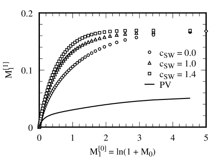
FIG. 2.: Plot of $M_{1}^{[1]}$ vs. $M_{1}^{[0]}$ for $c_{\text{SW}}=0$ (circles), 1 (triangles), and 1.4 (squares). The diamond marks the static limit [3]. To illustrate that the overall shape is not an artifact of lattice field theory, the curve shows $M_{\text{PV}}^{[1]}$. Here $C_{F}=4/3$.

We are able to reproduce the result of Ref. [21], which considers only the Wilson action, if we omit the tadpole diagram’s contribution $\Sigma^{[1]}_{\text{(b)}}$.

For $M_{1}a<1$ the additive form is not illuminating, because there $M_{1}^{[1]}\propto M_{1}^{[0]}$. It is convenient to define the rest-mass renormalization factor

$$Z_{M_{1}}\equiv\frac{M_{1}a}{\tanh M_{1}^{[0]}a}.$$ (82)

To build the one-loop renormalization factor from the vegas integrals let

$$z_{M_{1}}^{[1](n)}=e^{-M_{1}^{[0]}}\left(a_{0}^{[1](n)}\cosh M_{1}^{[0]}-c^{[1](n)}\coth M_{1}^{[0]}\right),$$ (83)

and then

$$Z_{M_{1}}^{[1](n)}=z_{M_{1}}^{[1](n)}+e^{-M_{1}^{[0]}}\cosh M_{1}^{[0]}\left[p_{A_{0}}^{(n)}(M_{1}^{{[0]}})A^{[1]}_{\text{PV}}-p_{C}^{(n)}(M_{1}^{{[0]}})B^{[1]}_{\text{PV}}\right].$$ (84)

Figure 3 shows the $z_{M_{1}}^{[1](n)}$ and Table I contains the first 15 coefficients of their Chebyshev expansions.

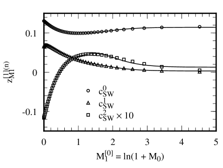
FIG. 3.: Plot of $z_{M_{1}}^{[1]}$ vs. $M_{1}^{[0]}$ as coefficients of $c_{\text{SW}}$. The curves indicate the fifteen-term Chebyshev interpolation. Note that $z_{M_{1}}^{[1](2)}$ (the coefficient of $c_{\text{SW}}^{2}$) is multiplied by ten. Here $C_{F}=4/3$.

TABLE I.: Coefficients of Chebyshev polynomials $T_{j}(x)$ for $z_{M_{1}}^{[1](n)}$. Here $C_{F}=4/3$.

$j$	$z_{M_{1}}^{[1](0)}$		$z_{M_{1}}^{[1](1)}$		$z_{M_{1}}^{[1](2)}$
0	0.	222802	0.	0868169	$-0$.	00278643
1	$-0$.	0117152	$-0$.	0300771	0.	00744513
2	0.	00883238	$-0$.	0052349	$-0$.	00297984
3	0.	00216047	$-0$.	000493063	$-0$.	00039969
4	0.	00141579	$-0$.	00245913	$-0$.	000478208
5	0.	000994781	$-0$.	000371327	$-0$.	000358493
6	0.	000590983	$-0$.	000965165	$-0$.	000237546
7	0.	000467076	$-0$.	000311904	$-0$.	000198283
8	0.	000321860	$-0$.	000497263	$-0$.	000147608
9	0.	000256113	$-0$.	000225545	$-0$.	000123028
10	0.	000195137	$-0$.	000302366	$-9$.	86053$\times 10^{-5}$
11	0.	000159702	$-0$.	000161754	$-8$.	34899$\times 10^{-5}$
12	0.	000125988	$-0$.	000203734	$-6$.	96978$\times 10^{-5}$
13	0.	000106567	$-0$.	000120868	$-5$.	99954$\times 10^{-5}$
14	8.	55174$\times 10^{-5}$	$-0$.	000146607	$-5$.	15038$\times 10^{-5}$
15	7.	61065$\times 10^{-5}$	$-9$.	24268$\times 10^{-5}$	$-4$.	50976$\times 10^{-5}$

In the massless limit there are several checks in the literature. As $M_{1}a\to 0$, we find

$$Z_{M_{1}}^{[1]}=C_{F}\left[0.10726(15)+0.04901(2)c_{\text{SW}}-0.008735(5)c_{\text{SW}}^{2}-\frac{3}{16\pi^{2}}\ln(M_{1}^{[0]}a)^{2}\right].$$ (85)

Note the appearance of the logarithm, multiplied by the one-loop anomalous dimension. The finite part agrees well with published values: $C_{F}0.107347(5)$ at $c_{\text{SW}}=0$ [9], and $C_{F}0.1474(4)$ at $c_{\text{SW}}=1$ [10]. The individual coefficients of $c_{\text{SW}}$ agree with Ref. [11].

Recently Sint and Weisz [14] have computed the next term in the expansion of $Z_{M_{1}}^{[1]}(M_{1}a)$ around $M_{1}a=0$, for $c_{\text{SW}}=1$. They find the coefficient of $M_{1}a$ to be $-C_{F}0.07217(2)$. Fitting our results for $M_{1}a<0.1$, we find $-C_{F}0.0720(7)$, less precise, but in agreement. Reference [14] does not report a contribution of order $M_{1}a\ln M_{1}a$; for $c_{\text{SW}}=1$ one would expect it to drop out. Our Pauli-Villars subtractions isolate from $Z_{M_{1}}^{[1](0)}$ a contribution $C_{F}[6/16\pi^{2}]M_{1}a\ln M_{1}a$, and our fits find nothing more of order $M_{1}a\ln M_{1}a$ in $Z_{M_{1}}^{[1](0)}$. But $Z_{M_{1}}^{[1](1)}$ contains precisely the same contribution with the opposite sign, so the total drops out when $c_{\text{S}W}=1$. This exercise verifies, as in Refs. [10, 11], that the tree-level improved action removes terms of order $a\ln a$.

These checks are reassuring, but the main result is the full mass dependence, embodied in Figs. 2 and 3 and in Table I. To proceed from our numerical results to $Z_{M_{1}}^{[1]}$:

1. reconstitute adequate approximations to the $z_{M_{1}}^{[1](n)}$ from Table I;

2. evaluate them at the desired value of $\tanh M_{1}^{[0]}$;

3. accumulate the polynomial in $c_{\text{SW}}$;

4. add $e^{-M_{1}^{[0]}}\cosh M_{1}^{[0]}(p_{A_{0}}A_{\text{PV}}-p_{C}B_{\text{PV}})$ to restore the Pauli-Villars subtraction.

The full one-loop approximation to the rest mass is then

$$M_{1}=M_{1}^{[0]}+g^{2}Z_{M_{1}}^{[1]}\tanh M_{1}^{[0]}.$$ (86)

In a straightforward application of bare perturbation theory the expansion parameter $g^{2}$ would be the bare coupling $g_{0}^{2}$. It is possible, however, to choose a better expansion parameter [18]. Further discussion of this issue will appear elsewhere.

C Kinetic Mass $M_{2}$

Figure 4 shows the one-loop renormalization of the kinetic mass for $c_{\text{SW}}=0$ and 1. (The variation with $c_{\text{SW}}$ is too weak to distinguish 1.4 from 1.) Again, $Z_{M_{2}}^{[1]}$ smoothly connects to the massless and static limits.

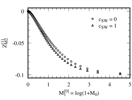
FIG. 4.: Plot of $Z_{M_{2}}^{[1]}$ vs. $M_{1}^{[0]}a$ for $c_{\text{SW}}=0$ (circles) and 1 (triangles). The diamond marks the static limit [12]. Here $C_{F}=4/3$.

The separate coefficients of $c_{\text{SW}}$ are plotted in Fig. 5, and their first fifteen Chebyshev coefficients are listed in Table II.

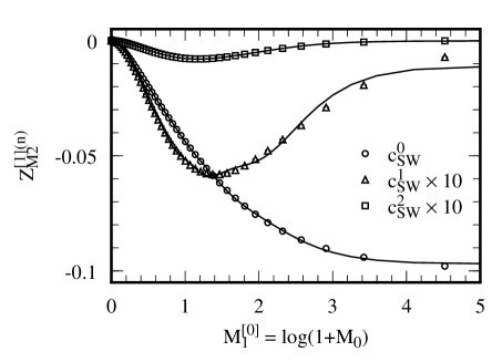
FIG. 5.: Plot of $Z_{M_{2}}^{[1](n)}$ vs. $M_{1}^{[0]}a$. The curves indicate the fifteen-term Chebyshev interpolation. Note that the coefficients of $c_{\text{SW}}^{1}$ and $c_{\text{SW}}^{2}$ are multiplied by ten. Here $C_{F}=4/3$.

TABLE II.: Coefficients of Chebyshev polynomials $T_{j}(x)$ for $Z_{M_{2}}^{[1](n)}$. Here $C_{F}=4/3$.

$j$	$Z_{M_{2}}^{[1](0)}$		$Z_{M_{2}}^{[1](1)}$		$Z_{M_{2}}^{[1](2)}$
0	$-$0.	0631437	$-$0.	00518218	$-$0.	000697017
1	$-$0.	0409363	$-$0.	00266278	$-$0.	000293363
2	$-$0.	0113513	0.	000649031	0.	000188227
3	$-$0.	00411835	0.	00104410	0.	000188092
4	$-$0.	00293037	0.	000578677	9.	36398$\times 10^{-5}$
5	$-$0.	00157589	0.	000435851	5.	85129$\times 10^{-5}$
6	$-$0.	00118956	0.	000331139	3.	40842$\times 10^{-5}$
7	$-$0.	00081670	0.	000251324	2.	23707$\times 10^{-5}$
8	$-$0.	000630783	0.	000204140	1.	47425$\times 10^{-5}$
9	$-$0.	000490657	0.	000162222	1.	02279$\times 10^{-5}$
10	$-$0.	000396438	0.	000137218	0.	71930$\times 10^{-5}$
11	$-$0.	000319830	0.	000112310	0.	52123$\times 10^{-5}$
12	$-$0.	000273443	9.	74213$\times 10^{-5}$	0.	39003$\times 10^{-5}$
13	$-$0.	000223656	8.	30367$\times 10^{-5}$	0.	29204$\times 10^{-5}$
14	$-$0.	000198908	7.	12494$\times 10^{-5}$	0.	21814$\times 10^{-5}$
15	$-$0.	000163911	6.	31163$\times 10^{-5}$	0.	17610$\times 10^{-5}$

In the static limit we find $Z_{M_{2}}^{[1]}(\infty)=-C_{F}0.0745(1)=-0.0993(1)$, which agrees with $-0.0998(4)$, the value in nonrelativistic QCD [12, 13] for our definition of $Z_{M_{2}}$. In the massless limit we verify $Z_{M_{2}}^{[1]}(0)=0$, because there $M_{2}=M_{1}$.

These checks are again reassuring, but the main result is the full mass dependence, embodied in Figs. 4 and 5 and in Table II. To proceed from our numerical results to $Z_{M_{2}}^{[1]}$:

1. reconstitute adequate approximations to the $Z_{M_{2}}^{[1](n)}$ from Table II;

2. evaluate them at the desired $\tanh M_{1}^{[0]}$;

3. accumulate the polynomial in $c_{\text{SW}}$.

The full one-loop approximation to the kinetic mass is then

$$M_{2}=m_{2}(M_{1}^{[0]}+g_{1}^{2}M_{1}^{[1]})\left(1+g_{2}^{2}Z_{M_{2}}^{[1]}\right).$$ (87)

Again, it may be appropriate to choose optimal expansion parameters $g_{1}^{2}$ and $g_{2}^{2}$, as will be discussed elsewhere.

D Wave-function Renormalization $Z_{2}$

Because the wave-function renormalization factor’s full correction $Z_{2}^{[1]}$ has an infrared divergence for all values of the quark mass, we present results for the subtracted form, as defined in Eq. (77). Figure 6 shows the one-loop correction $z_{2}^{[1]}$, in Feynman gauge, for $c_{\text{SW}}=0$, 1, and 1.4. Once again, $z_{2}^{[1]}$ smoothly connects the massless and static limits.

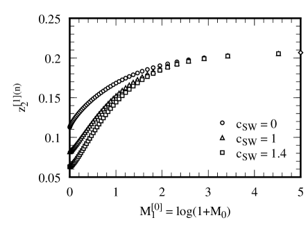
FIG. 6.: Plot of $z_{2}^{[1]}$ vs. $M_{1}^{[0]}$ for $c_{\text{SW}}=0$ (circles), 1 (triangles), and 1.4 (squares). The diamond marks the static limit [3]. Here $C_{F}=4/3$.

The separate coefficients of $c_{\text{SW}}$ are plotted in Fig. 7, and their first fifteen Chebyshev coefficients are listed in Table III.

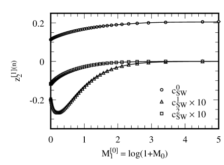
FIG. 7.: Plot of $z_{2}^{[1](n)}$ vs. $M_{1}^{[0]}a$. The curves indicate the fifteen-term Chebyshev interpolation. Note that the coefficients of $c_{\text{SW}}^{1}$ and $c_{\text{SW}}^{2}$ are multiplied by ten. Here $C_{F}=4/3$.

TABLE III.: Coefficients of Chebyshev polynomials $T_{j}(x)$ for $z_{2}^{[1](n)}$. Here $C_{F}=4/3$.

$j$	$z_{2}^{[1](0)}$		$z_{2}^{[1](1)}$		$z_{2}^{[1](2)}$
0	0.	305389	$-$0.	033722	$-$0.	0111230
1	0.	0392549	0.	0108371	0.	00554548
2	0.	00310868	0.	00597098	$-$0.	000324921
3	0.	00393177	$-$0.	00107846	0.	000324902
4	0.	00138399	0.	00096398	$-$1.	79973$\times 10^{-5}$
5	0.	00134333	$-$0.	000166528	2.	44776$\times 10^{-5}$
6	0.	000666205	0.	000233668	0.	38057$\times 10^{-5}$
7	0.	000655838	$-$4.	30696$\times 10^{-5}$	0.	283444$\times 10^{-5}$
8	0.	000391408	8.	67030$\times 10^{-5}$	0.	156463$\times 10^{-5}$
9	0.	000380178	$-$1.	79973$\times 10^{-5}$	0.	062247$\times 10^{-5}$
10	0.	000255127	4.	08834$\times 10^{-5}$	0.	038319$\times 10^{-5}$
11	0.	000252910	$-$1.	04220$\times 10^{-5}$	0.	020393$\times 10^{-5}$
12	0.	000181397	2.	24672$\times 10^{-5}$	0.	007974$\times 10^{-5}$
13	0.	000172181	$-$0.	68263$\times 10^{-5}$	0.	005127$\times 10^{-5}$
14	0.	000122340	1.	43152$\times 10^{-5}$	0.	001010$\times 10^{-5}$
15	0.	000120061	$-$0.	53572$\times 10^{-5}$	$-$0.	004476$\times 10^{-5}$

In the static limit we find $Z_{2}^{[1]}(\infty)+C_{F}[2/16\pi^{2}]\ln\lambda^{2}=C_{F}0.1548(5)=0.2064(7)$, which agrees with $0.2067(1)$, the value of Refs. [3, 12] for our definition of $Z_{2}$.

In the massless limit we find

$$Z_{2}^{[1]} = C_{F}\left[0.05608(7)-0.014239(6)c_{\text{SW}}-0.008844(3)c_{\text{SW}}^{2}\right.$$ (88)

$$+ \left.\left(3\ln(M_{1}^{[0]}a)^{2}-2\ln(\lambda a)^{2}\right)/16\pi^{2}\right].$$ (89)

Note the appearance of a logarithm of $M^{2}$ as well as the infrared divergence. The finite part agrees well with published values: $C_{F}0.056057(2)$ at $c_{\text{SW}}=0$ [9] and $C_{F}0.0329(3)$ at $c_{\text{SW}}=1$ [10]. The individual coefficients of $c_{\text{SW}}$ agree with Ref. [11]. For comparison with Figs. 6 and 7, note that though $z_{2}^{[1](0)}$ does not contain the logarithms, it is larger by $C_{F}[9/32\pi^{2}]$ than the finite part of $Z_{2}^{[1](0)}$.

Once again, the checks are reassuring, but the main result is the full mass dependence. In practice, the wave-function renormalization factor is used only combined with vertex renormalization factors, in ways such that the infrared divergences cancel. When calculating a vertex renormalization factor, one should isolate all infrared divergences analytically, as we have done here, and then assemble the pieces so that the cancellation is explicit. If one chooses an on-shell renormalization scheme, dependence on the gauge parameter should cancel as well.

VII Improved Perturbation Theory

The previous section presented results for the (mass-dependent) one-loop coefficients in Eqs. (55), (58), and (60). Truncating the series at one loop, without further ado, is unlikely to be a good approximation to the full series, however. The one-loop self energy is large, owing to the contribution of the tadpole diagram in Feynman gauge, $\Sigma^{[1]}_{\text{(b)}}$. This feature will persist at higher orders. Similarly, tadpole diagrams make the bare coupling $g_{0}^{2}$ much smaller than other, more physical measures of the gauge interaction. Thus, one must be wary of these series; they are characterized by an unusually small expansion parameter, counteracted by unusually large coefficients.

These observations suggest rearranging perturbation series so that tadpole diagrams cancel each other in final results [18]. The rearrangement is achieved by defining new couplings and (re)normalization factors. Wherever the gauge field appears in the action or in operators, substitute

$$U_{\mu}\to u_{0}[U_{\mu}/u_{0}],$$ (90)

where the new parameter $u_{0}$, the mean link, is a gauge-invariant average of the link matrices $U_{\mu}$. The perturbative expansion of $u_{0}$, like any involving $U_{\mu}$, is dominated by its tadpole diagram. In the perturbative expansion of $U_{\mu}/u_{0}$, on the other hand, the tadpole diagrams cancel. The price for arranging the cancellation is that the first factor of $u_{0}$ in Eq. (90) must be evaluated nonperturbatively.

In the following discussion we shall denote the tadpole-improved gauge coupling as $\tilde{g}^{2}$, without defining it explicitly. The definition of $\tilde{g}^{2}$ affects higher-order corrections and numerical evaluation of a series truncated at one loop (or beyond). But it does not affect the one-loop self energy, which is the main focus here. On the other hand, tadpole improvement of the bare mass and of the field normalization do alter the one-loop coefficients, and they are considered below.

A Rest Mass $M_{1}$

The rest mass is primarily sensitive to the bare mass, particularly the subtracted version, $M_{0}=m_{0}-m_{0c}$. To derive a tadpole-improved bare mass, it is easiest to apply Eq. (90) to the hopping-parameter form of the action. Our action $S_{0}$ [6] has two hopping parameters,

$$\kappa_{t}=\frac{1}{2[1+(d-1)r_{s}\zeta+m_{0}]}$$ (91)

for temporal hops and $\kappa_{s}=\zeta\kappa_{t}$ for spatial hops. After rescaling the fields by $\sqrt{2\kappa_{t}}$, the link matrices appear only in the combinations $\kappa_{t}U_{0}$ and $\kappa_{s}U_{i}$. In view of Eq. (90) one defines the tadpole-improved hopping parameters $\tilde{\kappa}_{t,s}=u_{0}\kappa_{t,s}$ to absorb the first factor of $u_{0}$. Undoing the rescaling, now with $\sqrt{2\tilde{\kappa}_{t}}$, and reassembling the mass form leads to

$$\tilde{M}_{0}\equiv\tilde{m}_{0}-\tilde{m}_{0c}=M_{0}/u_{0}.$$ (92)

The numerical value of the tadpole-improved mass $\tilde{M}_{0}$ relies on two nonperturbatively determined parameters, $m_{0c}$ and $u_{0}$.

This rearrangement does not alter Eq. (30). Before developing the perturbation series, however, one sets $M_{0}=u_{0}\tilde{M}_{0}$, treats $\tilde{M}_{0}$ as the variable independent of $\tilde{g}^{2}$, and expands the explicit $u_{0}$ as well as the self-energy functions. Thus,

$$M_{1}=\sum_{l=0}^{\infty}\tilde{g}^{2l}\tilde{M}_{1}^{[l]},$$ (93)

where $\tilde{M}_{1}^{[0]}=\ln(1+\tilde{M}_{0})$ and

$$\tilde{M}_{1}^{[1]}=M_{1}^{[1]}+\frac{\tilde{M}_{0}}{1+\tilde{M}_{0}}u_{0}^{[1]}.$$ (94)

Since $u_{0}^{[1]}$ is negative, the (positive) coefficient $M_{1}^{[1]}$ is reduced. Note also that the mass dependence of the tadpole improvement connects smoothly to the small- and large-mass limits.

To illustrate the efficacy of tadpole improvement we take the mean link to be $u_{0}=\langle U_{\Box}\rangle^{1/4}$, where $U_{\Box}$ denotes the product of link matrices around a plaquette, $u_{0}^{[1]}=-C_{F}/16$. Figure 8 shows explicitly that $\tilde{z}_{M_{1}}^{[1]}$ is significantly smaller than $z_{M_{1}}^{[1]}$, when $u_{0}$ is defined this way.

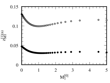
FIG. 8.: Plot comparing $z_{M_{1}}^{[1]}a$ vs. $M_{1}^{[1]}a$ (open symbols) and $\tilde{z}_{M_{1}}^{[1]}a$ vs. $\tilde{M}_{1}^{[1]}a$ (closed symbols). The static limit is indicated by diamonds [3].

(This choice of $u_{0}$ does not modify the terms proportional to $c_{\text{SW}}$ and $c_{\text{SW}}^{2}$.) For $c_{\text{SW}}=1$ the mass dependence at $Ma=0$ is also less steep: $-C_{F}[0.07217-1/32]=-C_{F}0.04088$. Other definitions of $u_{0}$ produce a qualitatively similar reduction.

B Kinetic Mass $M_{2}$

Because the kinetic-mass renormalization factor $Z_{M_{2}}$ is defined as a ratio of on-shell (and therefore physical) quantities, it should not be surprising that its one-loop correction $Z_{M_{2}}^{[1]}$ is unaffected by the tadpole diagram. More concretely, one can track analytically the contribution of $\Sigma^{[1]}_{(b)}$ through Eq. (59), to verify that it drops out (for all $M_{1}^{[0]}$). Thus, there are only two changes to improve the one-loop estimate of the kinetic mass: Use $\tilde{M}_{1}^{[0]}+\tilde{g}^{2}\tilde{M}_{1}^{[1]}$ as the argument of $m_{2}$ in Eq. (87), and use an improved coupling in the expansion of $Z_{M_{2}}$.

C Wave-function Renormalization $Z_{2}$

In the rescaling from the hopping-parameter form of the action to the mass form, the tadpole-improved version carries an additional factor of $u_{0}$, because $\tilde{\kappa}=u_{0}\kappa$. Thus, the renormalization factor of the tadpole-improved wave function is $\tilde{Z}_{2}=u_{0}Z_{2}$. Following Eq. (60) we develop the perturbative series

$$e^{M_{1}a}\tilde{Z}_{2}=1+\sum_{l=1}^{\infty}\tilde{g}^{2l}\tilde{Z}_{2}^{[l]}.$$ (95)

Comparing the expansions one easily finds

$$\tilde{Z}_{2}^{[1]}=Z_{2}^{[1]}+u_{0}^{[1]}.$$ (96)

Figure 9 compares $\tilde{z}_{2}^{[1]}=z_{2}^{[1]}+u_{0}^{[1]}$ to $z_{2}^{[1]}$ (in Feynman gauge). Once again, $\tilde{z}_{2}^{[1]}$ is significantly smaller.

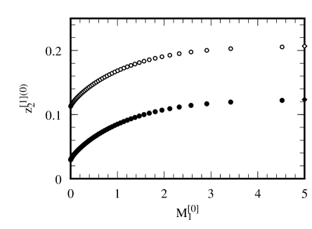
FIG. 9.: Plot comparing $z_{2}^{[1]}$ vs. $M_{1}^{[1]}a$ (open symbols) and $\tilde{z}_{2}^{[1]}$ vs. $\tilde{M}_{1}^{[1]}a$ (closed symbols).

VIII Conclusions

The work presented here is the first thorough study of renormalization in the approach of Ref. [6] to massive lattice fermions. (Some of our results have appeared earlier [15, 16, 17].) On the one hand, the specific, numerical results can be combined with Monte Carlo calculations of heavy-quark spectra to determine the heavy quarks’ masses. On the other hand, the techniques used to arrive at those results can be extended as the renormalization program is extended to vertex corrections. The most timely example of the latter is the renormalization of (improved) vector and axial-vector currents [22], which are needed to obtain heavy-light meson decay constants and semi-leptonic form factors.

The theoretical analysis of Sec. II examines renormalization to all orders in the gauge coupling and in the fermion mass. Although the focus is on the fermion propagator, the analysis serves as a model for the renormalization of currents as well. For currents one would introduce appropriate vertex functions, the analogs of the self-energy functions $A_{\rho}$ and $C$, again constrained only by periodicity and symmetry properties. Then one would Fourier transform the fourth component of each external momentum to obtain the on-shell correlation function (for quark states) to all orders in the mass and the gauge coupling. Just as here, the all-orders formulae would provide useful insights, and they would be convenient for developing expansions to any desired order.

In our numerical work we subtract from the self-energy functions corresponding functions from a Pauli-Villars regulator. In this way we are able to isolate mass and infrared singularities, including, for small $Ma$, contributions of the form $Ma\ln Ma$. The Pauli-Villars functions can be written in closed form, so we have analytical control of the singularities. Furthermore, by applying the subtraction at the integrand level, numerical integration of the nonsingular part is simplified. For example, one can carry out the integration without an infrared regulator. These techniques should continue to be helpful for the renormalization of currents and other operators.

The numerical results presented in Sec. VI demonstrates that the mass dependence of renormalization factors smoothly connects the massless and static limits. This was expected from the free theory and general arguments [6], but it is satisfying to make it explicit. Also expected, but now explicit, is the result in Sec. VII that tadpole improvement [18] reduces the size of the one-loop coefficients for all masses. In the case of the rest-mass renormalization factor, tadpole improvement also makes the mass dependence even smoother, cf. Fig. 8.

Our results, especially with tadpole improvement, will be useful in determining the $\overline{\rm MS}$ masses of heavy quarks [19]. Additionally, such a determination will require at least an evaluation of the optimal scale [18] (in progress), and, to achieve better than 5% accuracy, the complete two-loop calculation. Nevertheless, the approach taken here to the renormalization of massive lattice gauge theories is a necessary first step.

A Feynman Rules

This is the first paper to address perturbation theory for the action discussed in Sec. III, so we give here the propagators and vertices needed for the one-loop self energy. Figure 10 defines indices and momentum flow. Then

Fig. 10a $$= G_{0}(p)_{ij}=\frac{\delta_{ij}}{i\gamma_{0}\sin p_{0}+i\zeta\mathchoice{{\hbox{\boldmath$\displaystyle\gamma$}}}{{\hbox{\boldmath$\textstyle\gamma$}}}{{\hbox{\boldmath$\scriptstyle\gamma$}}}{{\hbox{\boldmath$\scriptscriptstyle\gamma$}}}\cdot\mathchoice{{\hbox{\boldmath$\displaystyle S$}}}{{\hbox{\boldmath$\textstyle S$}}}{{\hbox{\boldmath$\scriptstyle S$}}}{{\hbox{\boldmath$\scriptscriptstyle S$}}}(\mathchoice{{\hbox{\boldmath$\displaystyle p$}}}{{\hbox{\boldmath$\textstyle p$}}}{{\hbox{\boldmath$\scriptstyle p$}}}{{\hbox{\boldmath$\scriptscriptstyle p$}}})+1+m_{0}-\cos p_{0}+\frac{1}{2}r_{s}\zeta\hat{\mathchoice{{\hbox{\boldmath$\displaystyle p$}}}{{\hbox{\boldmath$\textstyle p$}}}{{\hbox{\boldmath$\scriptstyle p$}}}{{\hbox{\boldmath$\scriptscriptstyle p$}}}}^{2}},$$ (A1)

Fig. 10b $$= \Delta^{ab}_{\mu\nu}(k)=\frac{\delta^{ab}}{\hat{k}^{2}}\left(\delta_{\mu\nu}-(1-\alpha)\frac{\hat{k}_{\mu}\hat{k}_{\nu}}{\hat{k}^{2}}\right),$$ (A2)

Fig. 10c $$= -g_{0}t^{a}_{ij}[\gamma_{0}\cos\frac{1}{2}(p+p^{\prime})_{0}-i\sin\frac{1}{2}(p+p^{\prime})_{0}+\frac{1}{2}c_{E}\zeta\sigma_{0r}\cos\frac{1}{2}k_{0}\sin k_{r}],$$ (A3)

Fig. 10d $$= -g_{0}\zeta t^{a}_{ij}[\gamma_{m}\cos\frac{1}{2}{(p+p^{\prime})_{m}}-ir_{s}\sin\frac{1}{2}(p+p^{\prime})_{m}$$ (A4)

$$+ \frac{1}{2}c_{B}\sigma_{mn}\cos\frac{1}{2}k_{m}\sin k_{n}+\frac{1}{2}c_{E}\sigma_{m0}\cos\frac{1}{2}k_{m}\sin k_{0}],$$ (A5)

Fig. 10e $$= g_{0}^{2}\frac{1}{2}\{t^{a},t^{b}\}_{ij}[\cos\frac{1}{2}(p+p^{\prime})_{0}-i\gamma_{0}\sin\frac{1}{2}(p+p^{\prime})_{0}]$$ (A6)

$$- \frac{i}{4}g_{0}^{2}c_{E}\zeta[t^{a},t^{b}]_{ij}\sigma_{0r}(\sin k_{r}-\sin l_{r})\sin\frac{1}{2}(k+l)_{0},$$ (A7)

Fig. 10f $$= -\frac{i}{2}g_{0}^{2}c_{E}\zeta[t^{a},t^{b}]_{ij}\sigma_{0m}\times$$ (A9)

$$[2\cos\frac{1}{2}(k+l)_{0}\cos\frac{1}{2}(k+l)_{m}\cos\frac{1}{2}l_{0}\cos\frac{1}{2}k_{m}-\cos\frac{1}{2}l_{m}\cos\frac{1}{2}k_{0}],$$

Fig. 10g $$= \frac{1}{2}g_{0}^{2}\zeta\{t^{a},t^{b}\}_{ij}\delta_{mn}[r_{s}\cos\frac{1}{2}(p+p^{\prime})_{m}-i\gamma_{m}\sin\frac{1}{2}(p+p^{\prime})_{m}]$$ (A10)

$$- \frac{i}{2}g_{0}^{2}c_{B}\zeta[t^{a},t^{b}]_{ij}\sigma_{mn}\times$$ (A12)

$$[2\cos\frac{1}{2}(k+l)_{m}\cos\frac{1}{2}(k+l)_{n}\cos\frac{1}{2}l_{m}\cos\frac{1}{2}k_{n}-\cos\frac{1}{2}l_{n}\cos\frac{1}{2}k_{m}]$$

$$+ \frac{i}{4}g_{0}^{2}\zeta[t^{a},t^{b}]_{ij}\delta_{mn}\sin\frac{1}{2}(k+l)_{m}[c_{B}\sigma_{mr}(\sin k_{r}-\sin l_{r})+c_{E}\sigma_{m0}(\sin k_{0}-\sin l_{0})],$$ (A13)

where $S_{i}(p_{i})=\sin p_{i}$; $\alpha$ is the gauge parameter ($\alpha=1$ yields Feynman gauge); $g_{0}$ is the bare gauge coupling; the $t^{a}$ are (anti-Hermitian) generators of SU(3), normalized so that $\mathop{\rm tr}t^{a}t^{b}=-\delta^{ab}/2$; and the $\gamma$ matrix conventions are as in Ref. [6]. One can verify easily that these rules reduce to the ones for the Sheikholeslami-Wohlert action when $\zeta=1$, $r_{s}=1$, and $c_{B}=c_{E}$.

FIG. 10.: Feynman rules for the action $S_{0}+S_{B}+S_{E}$ defined in Sec. III.

B Numerators

It is convenient to sort the numerator $F(p,k)$ in Eq. (62) according to the number of clover interactions:

$$F=F_{0}+c_{B}F_{c_{B}}+c_{E}F_{c_{E}}+c_{B}^{2}F_{c_{B}^{2}}+c_{B}c_{E}F_{c_{B}c_{E}}+c_{E}^{2}F_{c_{E}^{2}}.$$ (B1)

The Wilson-action term $F_{0}$ is gauge dependent, but the other terms are independent of the gauge parameter. Below we give $F_{0}$ in Feynman gauge [$\alpha=1$ in Eq. (A2)]. The sum of internal quark and gluon momenta appears often, so let $s=p+(p+k)=2p+k$. From the Feynman rules, tedious algebra (performed by Mathematica and checked by hand) yields

$$F_{0}(p,k) = i\gamma_{0}\left[\sin(p+k)_{0}\{\cos s_{0}-\zeta^{2}[d-1+\frac{1}{4}(r_{s}^{2}-1)\hat{\mathchoice{{\hbox{\boldmath$\displaystyle s$}}}{{\hbox{\boldmath$\textstyle s$}}}{{\hbox{\boldmath$\scriptstyle s$}}}{{\hbox{\boldmath$\scriptscriptstyle s$}}}}^{2}]\}+L(p+k)\sin s_{0}\right]$$ (B2)

$$+ i\zeta\sum_{i}\gamma_{i}\left[\sin(p+k)_{i}\left(\zeta^{2}\{\cos s_{i}-[d-1+\frac{1}{4}(r_{s}^{2}-1)\hat{\mathchoice{{\hbox{\boldmath$\displaystyle s$}}}{{\hbox{\boldmath$\textstyle s$}}}{{\hbox{\boldmath$\scriptstyle s$}}}{{\hbox{\boldmath$\scriptscriptstyle s$}}}}^{2}]\}+\zeta^{2}-1\right)\right.$$ (B4)

$$\left.\hskip 71.13188pt\rule{0.0pt}{10.00002pt}+r_{s}\zeta L(p+k)\sin s_{i}\right]$$

$$+ \sin s_{0}\sin(p+k)_{0}+r_{s}\zeta^{3}\sin\mathchoice{{\hbox{\boldmath$\displaystyle s$}}}{{\hbox{\boldmath$\textstyle s$}}}{{\hbox{\boldmath$\scriptstyle s$}}}{{\hbox{\boldmath$\scriptscriptstyle s$}}}\cdot\sin(\mathchoice{{\hbox{\boldmath$\displaystyle p$}}}{{\hbox{\boldmath$\textstyle p$}}}{{\hbox{\boldmath$\scriptstyle p$}}}{{\hbox{\boldmath$\scriptscriptstyle p$}}}+\mathchoice{{\hbox{\boldmath$\displaystyle k$}}}{{\hbox{\boldmath$\textstyle k$}}}{{\hbox{\boldmath$\scriptstyle k$}}}{{\hbox{\boldmath$\scriptscriptstyle k$}}})$$ (B5)

$$- L(p+k)\{\cos s_{0}+\zeta^{2}[d-1-\frac{1}{4}(r_{s}^{2}+1)\hat{\mathchoice{{\hbox{\boldmath$\displaystyle s$}}}{{\hbox{\boldmath$\textstyle s$}}}{{\hbox{\boldmath$\scriptstyle s$}}}{{\hbox{\boldmath$\scriptscriptstyle s$}}}}^{2}]\},$$ (B6)

where $\hat{\mathchoice{{\hbox{\boldmath$\displaystyle q$}}}{{\hbox{\boldmath$\textstyle q$}}}{{\hbox{\boldmath$\scriptstyle q$}}}{{\hbox{\boldmath$\scriptscriptstyle q$}}}}^{2}=\sum_{i}(2\sin\frac{1}{2}q_{i})^{2}$, and $L(q)=1+m_{0}a+\frac{1}{2}r_{s}\zeta\hat{\mathchoice{{\hbox{\boldmath$\displaystyle q$}}}{{\hbox{\boldmath$\textstyle q$}}}{{\hbox{\boldmath$\scriptstyle q$}}}{{\hbox{\boldmath$\scriptscriptstyle q$}}}}^{2}-\cos q_{0}$;

$$F_{c_{B}} = ir_{s}\zeta^{3}\sum_{j\neq i}[\gamma_{i}\sin(p+k)_{j}-\gamma_{j}\sin(p+k)_{i}]\sin k_{i}\sin\frac{1}{2}s_{j}\cos\frac{1}{2}k_{j}$$ (B7)

$$- i\zeta^{2}L(p+k)\sum_{j\neq i}\gamma_{i}\sin k_{i}\cos\frac{1}{2}k_{j}\cos\frac{1}{2}s_{j}+\zeta^{3}\sum_{j\neq i}\sin k_{i}\sin(p+k)_{i}\cos\frac{1}{2}k_{j}\cos\frac{1}{2}s_{j};$$ (B8)

$$F_{c_{E}} = ir_{s}\zeta^{3}\gamma_{0}\sin k_{0}\sum_{i}\cos\frac{1}{2}k_{i}\sin\frac{1}{2}s_{i}\sin(p+k)_{i}$$ (B9)

$$- i\zeta^{2}\gamma_{0}\left[\sin\frac{1}{2}s_{0}\cos\frac{1}{2}k_{0}\sin\mathchoice{{\hbox{\boldmath$\displaystyle k$}}}{{\hbox{\boldmath$\textstyle k$}}}{{\hbox{\boldmath$\scriptstyle k$}}}{{\hbox{\boldmath$\scriptscriptstyle k$}}}\cdot\sin(\mathchoice{{\hbox{\boldmath$\displaystyle p$}}}{{\hbox{\boldmath$\textstyle p$}}}{{\hbox{\boldmath$\scriptstyle p$}}}{{\hbox{\boldmath$\scriptscriptstyle p$}}}+\mathchoice{{\hbox{\boldmath$\displaystyle k$}}}{{\hbox{\boldmath$\textstyle k$}}}{{\hbox{\boldmath$\scriptstyle k$}}}{{\hbox{\boldmath$\scriptscriptstyle k$}}})+\sin k_{0}L(p+k)\sum_{i}\cos\frac{1}{2}k_{i}\cos\frac{1}{2}s_{i}\right]$$ (B10)

$$+ i\zeta\mathchoice{{\hbox{\boldmath$\displaystyle\gamma$}}}{{\hbox{\boldmath$\textstyle\gamma$}}}{{\hbox{\boldmath$\scriptstyle\gamma$}}}{{\hbox{\boldmath$\scriptscriptstyle\gamma$}}}\cdot\sin\mathchoice{{\hbox{\boldmath$\displaystyle k$}}}{{\hbox{\boldmath$\textstyle k$}}}{{\hbox{\boldmath$\scriptstyle k$}}}{{\hbox{\boldmath$\scriptscriptstyle k$}}}\cos\frac{1}{2}k_{0}[\sin(p+k)_{0}\sin\frac{1}{2}s_{0}-L(p+k)\cos\frac{1}{2}s_{0}]$$ (B11)

$$- ir_{s}\zeta^{2}\sin k_{0}\sin(p+k)_{0}\sum_{i}\gamma_{i}\cos\frac{1}{2}k_{i}\sin\frac{1}{2}s_{i}$$ (B12)

$$+ \zeta^{2}\sin\mathchoice{{\hbox{\boldmath$\displaystyle k$}}}{{\hbox{\boldmath$\textstyle k$}}}{{\hbox{\boldmath$\scriptstyle k$}}}{{\hbox{\boldmath$\scriptscriptstyle k$}}}\cdot\sin(\mathchoice{{\hbox{\boldmath$\displaystyle p$}}}{{\hbox{\boldmath$\textstyle p$}}}{{\hbox{\boldmath$\scriptstyle p$}}}{{\hbox{\boldmath$\scriptscriptstyle p$}}}+\mathchoice{{\hbox{\boldmath$\displaystyle k$}}}{{\hbox{\boldmath$\textstyle k$}}}{{\hbox{\boldmath$\scriptstyle k$}}}{{\hbox{\boldmath$\scriptscriptstyle k$}}})\cos\frac{1}{2}k_{0}\cos\frac{1}{2}s_{0}+\zeta^{2}\sin k_{0}\sin(p+k)_{0}\sum_{i}\cos\frac{1}{2}k_{i}\cos\frac{1}{2}s_{i};$$ (B13)

$$F_{c_{B}^{2}} = -\frac{i}{4}\zeta^{2}\gamma_{0}\sin(p+k)_{0}\sum_{j\neq i}\sin^{2}k_{i}\cos^{2}\frac{1}{2}k_{j}$$ (B14)

$$+ \frac{i}{2}\zeta^{3}\mathchoice{{\hbox{\boldmath$\displaystyle\gamma$}}}{{\hbox{\boldmath$\textstyle\gamma$}}}{{\hbox{\boldmath$\scriptstyle\gamma$}}}{{\hbox{\boldmath$\scriptscriptstyle\gamma$}}}\cdot\sin\mathchoice{{\hbox{\boldmath$\displaystyle k$}}}{{\hbox{\boldmath$\textstyle k$}}}{{\hbox{\boldmath$\scriptstyle k$}}}{{\hbox{\boldmath$\scriptscriptstyle k$}}}\sum_{j\neq i}\sin k_{i}\sin(p+k)_{i}\cos^{2}\frac{1}{2}k_{j}-\frac{i}{4}\zeta^{3}\mathchoice{{\hbox{\boldmath$\displaystyle\gamma$}}}{{\hbox{\boldmath$\textstyle\gamma$}}}{{\hbox{\boldmath$\scriptstyle\gamma$}}}{{\hbox{\boldmath$\scriptscriptstyle\gamma$}}}\cdot\sin(\mathchoice{{\hbox{\boldmath$\displaystyle p$}}}{{\hbox{\boldmath$\textstyle p$}}}{{\hbox{\boldmath$\scriptstyle p$}}}{{\hbox{\boldmath$\scriptscriptstyle p$}}}+\mathchoice{{\hbox{\boldmath$\displaystyle k$}}}{{\hbox{\boldmath$\textstyle k$}}}{{\hbox{\boldmath$\scriptstyle k$}}}{{\hbox{\boldmath$\scriptscriptstyle k$}}})\sum_{j\neq i}\sin^{2}k_{i}\cos^{2}\frac{1}{2}k_{j}$$ (B15)

$$+ \frac{i}{2}\zeta^{3}\sum_{{j\neq i}}\gamma_{i}\cos^{2}\frac{1}{2}k_{i}\sin k_{j}[\sin(p+k)_{i}\sin k_{j}-\sin(p+k)_{j}\sin k_{i}]$$ (B16)

$$+ \frac{1}{4}\zeta^{2}L(p+k)\sum_{j\neq i}\sin^{2}k_{i}\cos^{2}\frac{1}{2}k_{j};$$ (B17)

$$F_{c_{E}c_{B}}=\frac{i}{2}\zeta^{3}\gamma_{0}\sin k_{0}\sum_{j\neq i}\sin(p+k)_{i}\sin k_{i}\cos^{2}\frac{1}{2}k_{j}+\frac{i}{2}\zeta^{2}\sin(p+k)_{0}\sin k_{0}\sum_{j\neq i}\gamma_{i}\sin k_{i}\cos^{2}\frac{1}{2}k_{j};$$ (B18)

$$F_{c_{E}^{2}} = \frac{1}{4}\zeta^{2}\left[i\gamma_{0}\sin(p+k)_{0}-i\zeta\mathchoice{{\hbox{\boldmath$\displaystyle\gamma$}}}{{\hbox{\boldmath$\textstyle\gamma$}}}{{\hbox{\boldmath$\scriptstyle\gamma$}}}{{\hbox{\boldmath$\scriptscriptstyle\gamma$}}}\cdot\sin(\mathchoice{{\hbox{\boldmath$\displaystyle p$}}}{{\hbox{\boldmath$\textstyle p$}}}{{\hbox{\boldmath$\scriptstyle p$}}}{{\hbox{\boldmath$\scriptscriptstyle p$}}}+\mathchoice{{\hbox{\boldmath$\displaystyle k$}}}{{\hbox{\boldmath$\textstyle k$}}}{{\hbox{\boldmath$\scriptstyle k$}}}{{\hbox{\boldmath$\scriptscriptstyle k$}}})+L(p+k)\right]\times$$ (B20)

$$\hskip 71.13188pt\left[\cos^{2}\frac{1}{2}k_{0}\sum_{i}\sin^{2}k_{i}+\sin^{2}k_{0}\sum_{i}\cos^{2}\frac{1}{2}k_{i}\right]$$

$$+ \frac{i}{2}\zeta^{3}\left[(\mathchoice{{\hbox{\boldmath$\displaystyle\gamma$}}}{{\hbox{\boldmath$\textstyle\gamma$}}}{{\hbox{\boldmath$\scriptstyle\gamma$}}}{{\hbox{\boldmath$\scriptscriptstyle\gamma$}}}\cdot\sin\mathchoice{{\hbox{\boldmath$\displaystyle k$}}}{{\hbox{\boldmath$\textstyle k$}}}{{\hbox{\boldmath$\scriptstyle k$}}}{{\hbox{\boldmath$\scriptscriptstyle k$}}})[\sin\mathchoice{{\hbox{\boldmath$\displaystyle k$}}}{{\hbox{\boldmath$\textstyle k$}}}{{\hbox{\boldmath$\scriptstyle k$}}}{{\hbox{\boldmath$\scriptscriptstyle k$}}}\cdot\sin(\mathchoice{{\hbox{\boldmath$\displaystyle p$}}}{{\hbox{\boldmath$\textstyle p$}}}{{\hbox{\boldmath$\scriptstyle p$}}}{{\hbox{\boldmath$\scriptscriptstyle p$}}}+\mathchoice{{\hbox{\boldmath$\displaystyle k$}}}{{\hbox{\boldmath$\textstyle k$}}}{{\hbox{\boldmath$\scriptstyle k$}}}{{\hbox{\boldmath$\scriptscriptstyle k$}}})]\cos^{2}\frac{1}{2}k_{0}+\sin^{2}k_{0}\sum_{i}\gamma_{i}\sin(p+k)_{i}\cos^{2}\frac{1}{2}k_{i}\right].$$ (B21)

C Integration over Loop Momentum

To apply Eqs. (44), (27), and (33), one must obtain the self-energy functions $A_{\rho}$ and $C$ for real $p_{0}$ and analytically continue them to imaginary values $iE$. The analytical continuation must be approached cautiously in the representation of the self-energy functions as integrals over the loop variable $k_{0}$. The subtleties arise even with the continuum self energy. Setting the internal quark momentum to $q$, one has

$$\Sigma^{{[1]}}(p)=C_{F}\int\frac{d^{d}q}{(2\pi)^{d}}\,\frac{dm+i(d-2)\kern 1.00006pt/\kern-5.50003ptq}{(p-q)^{2}(q^{2}+m^{2})}.$$ (C1)

In the complex $q_{0}$ plane there are poles at $\pm iE(\mathchoice{{\hbox{\boldmath$\displaystyle q$}}}{{\hbox{\boldmath$\textstyle q$}}}{{\hbox{\boldmath$\scriptstyle q$}}}{{\hbox{\boldmath$\scriptscriptstyle q$}}})$ and at $p_{0}\pm i|\mathchoice{{\hbox{\boldmath$\displaystyle p$}}}{{\hbox{\boldmath$\textstyle p$}}}{{\hbox{\boldmath$\scriptstyle p$}}}{{\hbox{\boldmath$\scriptscriptstyle p$}}}-\mathchoice{{\hbox{\boldmath$\displaystyle q$}}}{{\hbox{\boldmath$\textstyle q$}}}{{\hbox{\boldmath$\scriptstyle q$}}}{{\hbox{\boldmath$\scriptscriptstyle q$}}}|$. (Here, in the continuum, $E(\mathchoice{{\hbox{\boldmath$\displaystyle q$}}}{{\hbox{\boldmath$\textstyle q$}}}{{\hbox{\boldmath$\scriptstyle q$}}}{{\hbox{\boldmath$\scriptscriptstyle q$}}})=\sqrt{\mathchoice{{\hbox{\boldmath$\displaystyle q$}}}{{\hbox{\boldmath$\textstyle q$}}}{{\hbox{\boldmath$\scriptstyle q$}}}{{\hbox{\boldmath$\scriptscriptstyle q$}}}^{2}+m^{2}}$.) The integration contour is the real axis. If one sets $p_{0}=iE(\mathchoice{{\hbox{\boldmath$\displaystyle p$}}}{{\hbox{\boldmath$\textstyle p$}}}{{\hbox{\boldmath$\scriptstyle p$}}}{{\hbox{\boldmath$\scriptscriptstyle p$}}})$, however, pole at $p_{0}-i|\mathchoice{{\hbox{\boldmath$\displaystyle p$}}}{{\hbox{\boldmath$\textstyle p$}}}{{\hbox{\boldmath$\scriptstyle p$}}}{{\hbox{\boldmath$\scriptscriptstyle p$}}}-\mathchoice{{\hbox{\boldmath$\displaystyle q$}}}{{\hbox{\boldmath$\textstyle q$}}}{{\hbox{\boldmath$\scriptstyle q$}}}{{\hbox{\boldmath$\scriptscriptstyle q$}}}|$ crosses into the upper half-plane when $|\mathchoice{{\hbox{\boldmath$\displaystyle p$}}}{{\hbox{\boldmath$\textstyle p$}}}{{\hbox{\boldmath$\scriptstyle p$}}}{{\hbox{\boldmath$\scriptscriptstyle p$}}}-\mathchoice{{\hbox{\boldmath$\displaystyle q$}}}{{\hbox{\boldmath$\textstyle q$}}}{{\hbox{\boldmath$\scriptstyle q$}}}{{\hbox{\boldmath$\scriptscriptstyle q$}}}|<E(\mathchoice{{\hbox{\boldmath$\displaystyle p$}}}{{\hbox{\boldmath$\textstyle p$}}}{{\hbox{\boldmath$\scriptstyle p$}}}{{\hbox{\boldmath$\scriptscriptstyle p$}}})$, and the contour must be deformed to accommodate it. Numerical integration packages are not clever enough to deform the contour; it is usually the real axis by default.

A better choice is to let $q=p+k$. In the complex $k_{0}$ plane the poles are at $-p_{0}\pm iE(\mathchoice{{\hbox{\boldmath$\displaystyle p$}}}{{\hbox{\boldmath$\textstyle p$}}}{{\hbox{\boldmath$\scriptstyle p$}}}{{\hbox{\boldmath$\scriptscriptstyle p$}}}+\mathchoice{{\hbox{\boldmath$\displaystyle k$}}}{{\hbox{\boldmath$\textstyle k$}}}{{\hbox{\boldmath$\scriptstyle k$}}}{{\hbox{\boldmath$\scriptscriptstyle k$}}})$ and $\pm i|\mathchoice{{\hbox{\boldmath$\displaystyle k$}}}{{\hbox{\boldmath$\textstyle k$}}}{{\hbox{\boldmath$\scriptstyle k$}}}{{\hbox{\boldmath$\scriptscriptstyle k$}}}|$. Then setting $p_{0}=iE(\mathchoice{{\hbox{\boldmath$\displaystyle p$}}}{{\hbox{\boldmath$\textstyle p$}}}{{\hbox{\boldmath$\scriptstyle p$}}}{{\hbox{\boldmath$\scriptscriptstyle p$}}})$ moves a pole across the real axis if $|\mathchoice{{\hbox{\boldmath$\displaystyle p$}}}{{\hbox{\boldmath$\textstyle p$}}}{{\hbox{\boldmath$\scriptstyle p$}}}{{\hbox{\boldmath$\scriptscriptstyle p$}}}|>|\mathchoice{{\hbox{\boldmath$\displaystyle p$}}}{{\hbox{\boldmath$\textstyle p$}}}{{\hbox{\boldmath$\scriptstyle p$}}}{{\hbox{\boldmath$\scriptscriptstyle p$}}}+\mathchoice{{\hbox{\boldmath$\displaystyle k$}}}{{\hbox{\boldmath$\textstyle k$}}}{{\hbox{\boldmath$\scriptstyle k$}}}{{\hbox{\boldmath$\scriptscriptstyle k$}}}|$. For the wave function and the rest mass, one wants external momentum $\mathchoice{{\hbox{\boldmath$\displaystyle p$}}}{{\hbox{\boldmath$\textstyle p$}}}{{\hbox{\boldmath$\scriptstyle p$}}}{{\hbox{\boldmath$\scriptscriptstyle p$}}}=\mathchoice{{\hbox{\boldmath$\displaystyle 0$}}}{{\hbox{\boldmath$\textstyle 0$}}}{{\hbox{\boldmath$\scriptstyle 0$}}}{{\hbox{\boldmath$\scriptscriptstyle 0$}}}$, so the pole cannot, in fact, cross. When the quark mass is large, however, the pole comes very close to the real axis, producing a sharp peak near $k_{0}=0$. Such integrals are difficult to estimate robustly. Even worse are the derivatives needed for the combination $D$, cf. Eq. (34): partial differentiation with respect to $p_{1}$ and $p_{0}$ each induces infrared divergences, which must, however, cancel in the total derivative.

Consequently, it is prudent, if cumbersome, to integrate over $k_{0}$ analytically [3, 12, 13]. The easiest way is contour integration. In a lattice theory, one can proceed as follows, see Fig. 11a. One is to integrate on the real axis over the interval $[-\pi,\pi]$. At $\pm\pi$ one extends the contour vertically to $\pm\pi+i\infty$. Then one closes the contour with a segment from $\pi+i\infty$ to $-\pi+i\infty$, resulting in a rectangular contour.

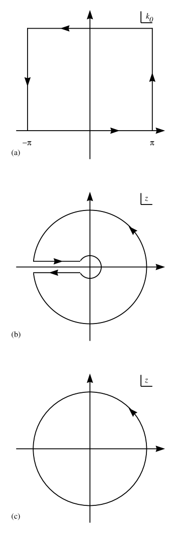
FIG. 11.: Contours for integrating over $k_{0}$. (a) The complex $k_{0}$ plane; (b) conformal map of onto the complex $z$ plane; (c) the final contour in the complex $z$ plane.

Since the integrand is a periodic function of $k_{0}$, the contributions from the two vertical sides cancel. For the Wilson action, the contribution from the top vanishes; for improved actions, however, this need not be the case; then the top must be subtracted out explicitly. This can be done elegantly by the conformal mapping $z=e^{ik_{0}}$. The rectangular contour maps into the contour shown in Fig. 11b. The top of the rectangle maps into the small circle around the origin; whether it needs to be subtracted back out, or not, it is always correct to take only the outer circle at $|z|=1$. The final contour is shown in Fig. 11c.

As a function of $z$ the integrand has poles at physical locations and at the origin. The latter restore the contribution from a nonvanishing “top of the rectangle.” It is then straightforward to integrate over $k_{0}$ for all forms of $k_{0}$ dependence appearing in Eqs. (B6)–(B21).

D Pauli-Villars Functions

Here we give explicit expressions for the self-energy functions with the Pauli-Villars regulator. They are needed to reconstruct the lattice results from the coefficients in the tables.

After introducing Feynman parameters and performing textbook manipulations one obtains

$$\Sigma^{[1]}_{\text{PV}}(p^{2};m)=-\frac{C_{F}}{16\pi^{2}}\int_{0}^{1}dx\,(4m+2ix\kern 1.00006pt/\kern-5.50003ptp)\;\ln\frac{\Delta_{1}(x)}{\Delta_{\lambda}(x)},$$ (D1)

where

$$\Delta_{\lambda}(x)=x\lambda^{2}+(1-x)m^{2}+x(1-x)p^{2}.$$ (D2)

Carrying out the integration over $x$ and setting $\lambda\to 0$, one finds

$$A^{[1]}_{\text{PV}}(-m^{2};m)=-\frac{C_{F}}{16\pi^{2}}\frac{1}{m^{2}}\left[(1-2m^{2})\varphi(m^{2})+1-\ln m^{2}\right],$$ (D3)

and, recalling Eq. (67),

$$B^{[1]}_{\text{PV}}(-m^{2};m)=4\frac{C_{F}}{16\pi^{2}}\varphi(m^{2})$$ (D4)

where

$$\varphi(m^{2})=\left\{\begin{array}[]{ll}m^{-2}\left(\frac{1}{2}\ln m^{2}+\sqrt{1-4m^{2}}\tanh^{-1}\sqrt{1-4m^{2}}\right),&m^{2}<\frac{1}{4}\\[10.00002pt] m^{-2}\left(\frac{1}{2}\ln m^{2}-\sqrt{4m^{2}-1}\tan^{-1}\sqrt{4m^{2}-1}\right),&m^{2}>\frac{1}{4}\end{array}\right..$$ (D5)

As $m^{2}\to 0$, $\varphi(m^{2})\to-1+\ln m^{2}+m^{2}(\frac{1}{2}+\ln m^{2})$; as $m^{2}\to\infty$, $\varphi(m^{2})\to-\pi/m$. Differentiating with respect to $p_{0}$, one finds

$$m\dot{A}^{[1]}_{\text{PV}}(-m^{2};m)=-4\frac{C_{F}}{16\pi^{2}}\left[\xi(m^{2})+\frac{1}{2}\ln(\lambda^{2}/m^{2})\right]$$ (D6)

$$m\dot{B}^{[1]}_{\text{PV}}(-m^{2};m)=-8\frac{C_{F}}{16\pi^{2}}\left[\eta(m^{2})+\frac{1}{2}\ln(\lambda^{2}/m^{2})\right]$$ (D7)

where

$$\xi(m^{2})=m^{-2}(1-\ln m^{2})-(1-m^{-2})\varphi(m^{2})+\psi(m^{2}),$$ (D8)

$$\eta(m^{2})=\ln m^{2}-\varphi(m^{2})-\psi(m^{2}),$$ (D9)

with

$$\psi(m^{2})=\frac{1}{2}\ln m^{2}+\left\{\begin{array}[]{ll}(1-4m^{2})^{-1/2}\tanh^{-1}\sqrt{1-4m^{2}},&m^{2}<\frac{1}{4}\\[10.00002pt] (4m^{2}-1)^{-1/2}\tan^{-1}\sqrt{4m^{2}-1},&m^{2}>\frac{1}{4}\end{array}\right..$$ (D10)

As $m^{2}\to 0$, $\psi(m^{2})\to-m^{2}(\ln m^{2}+1)$; as $m^{2}\to\infty$, $\psi(m^{2})\to\frac{1}{2}\ln m^{2}$.

REFERENCES

- [1] B. J. Gough, et al., Phys. Rev. Lett. 79, 1622 (1997).
- [2] E. Eichten, Nucl. Phys. B Proc. Suppl. 4, 170 (1988).
- [3] E. Eichten and B. Hill, Phys. Lett. B240, 193 (1990).
- [4] W. E. Caswell and G. P. Lepage, Phys. Lett. 167B, 437 (1986).
-
[5]
G. P. Lepage and B. A. Thacker,
Nucl. Phys. B Proc. Suppl. 4, 199 (1988);
B. A. Thacker and G. P. Lepage, Phys. Rev. D43, 196 (1991);
G. P. Lepage, et al., Phys. Rev. D46, 196 (1992). - [6] A. X. El-Khadra, A. S. Kronfeld, and P. B. Mackenzie, Phys. Rev. D55, 3933 (1997).
- [7] K. G. Wilson, in New Phenomena in Subnuclear Physics, edited by A. Zichichi (Plenum, New York, 1977).
- [8] B. Sheikholeslami and R. Wohlert, Nucl. Phys. B259, 572 (1985).
- [9] R. Groot, J. Hoek, and J. Smit, Nucl. Phys. B237, 111 (1984).
-
[10]
E. Gabrielli, et al., Nucl. Phys. B362, 475 (1991);
A. Borrelli, C. Pittori, R. Frezzotti, and E. Gabrielli, Nucl. Phys. B409, 382 (1993). - [11] S. Capitani, et al., DESY 97-181 (hep-lat/9709049); DESY 97-216 (hep-lat/ 9711007).
- [12] C. T. H. Davies and B. A. Thacker, Phys. Rev. D45, 915 (1992).
- [13] C. Morningstar, Phys. Rev. D48, 2265 (1993); D50, 5902 (1994).
- [14] S. Sint and P. Weisz, Nucl. Phys. B502, 251 (1997).
- [15] A. S. Kronfeld and B. P. Mertens, Nucl. Phys. B Proc. Suppl. 34, 495 (1994).
- [16] A. X. El-Khadra and B. P. Mertens, Nucl. Phys. B Proc. Suppl. 42, 406 (1995).
- [17] B. P. G. Mertens, University of Chicago Ph. D. Thesis, unpublished (1997).
- [18] G. P. Lepage and P. B. Mackenzie, Phys. Rev. D48, 2265 (1993).
- [19] For a preliminary look at , see A. S. Kronfeld, FERMILAB-CONF-97/326-T (hep-lat/9710007).
- [20] K. G. Wilson, Phys. Rev. D10, 2445 (1974).
- [21] Y. Kuramashi, KEK-CP-55 (hep-lat/9705036).
- [22] S. Aoki, S. Hashimoto, K.-I. Ishikawa, and T. Onogi, in preparation.