1 Introduction

The Atiyah-Singer index theorem [2] is considered to be among the greatest achievements of differential geometry. It has entered the physics literature in many places. Of particular interest is its application in gauge theories with fermions. The Atiyah-Singer index theorem relates the topological charge $\nu[A]$ of a sufficiently smooth gauge field configuration $A$ to the index of the Dirac operator on some compact manifold (or for gauge fields with suitable boundary conditions). The index of the operator can be expressed as the difference of the number of (lineraly independent) negative ($n_{-}$) and positive ($n_{+}$) chirality zero modes. The zero modes are eigenstates of the Dirac operator with eigenvalue $E=0$. Since $\gamma_{5}$ anti-commutes with $i\hbox to0.0pt{D\hss}{\not}\;\;$, the zero modes can be chosen as eigenstates $\psi_{+},\psi_{-}$ of $\gamma_{5}$ with $\gamma_{5}\psi_{+}=+\psi_{+}$ and $\gamma_{5}\psi_{-}=-\psi_{-}$. $n_{+}$ ($n_{-}$) denotes the number of independent states $\psi_{+}$ ($\psi_{-}$). The Atiyah-Singer index theorem [2] then reads

$$\nu[A]\;=\;n_{-}\;-\;n_{+}\;\;\;\;.$$ (1)

This relation allows to relate properties of fermionic observables to the topology of the background gauge field. Unfortunately, the gauge fields carrying the measure of the continuum path integral do not obey the necessary smoothnes condition [3] for the index theorem to apply in the fully quantized theory. The application of the index theorem is thus restricted to semiclassical arguments.

On the lattice the situation is different. It is possible to assign a topological charge to all gauge field configurations (see e.g. [4] for a recent review), up to so-called exceptional configurations which do not contribute in the continuum limit. The lattice path integral for the gauge fields thus effectively can be decomposed into topological sectors. Certainly it would be valuable to be able to understand the behavior of fermionic observables in each sector. Unfortunately there is no analytic result for an index theorem on the lattice. However, many contributions can be found in the literature [5] - [26], where a probabilistic manifestation of the Atiyah-Singer index theorem on the lattice and its consequences are discussed.

The pioneering papers [5, 6, 7] investigated the manifestation of the index theorem on the lattice by analyzing the pseudoscalar density operator which through chiral Ward identities can be related to the topological charge. In two interesting papers by Smit and Vink [8] these relations were extended to a lattice version of the Witten-Veneziano formula for the pseudoscalar masses. In two numerical studies [9] the interplay between pseudoscalar density operators and the topological charge was further investigated for two-dimensional models. Complete spectra of the Wilson-Dirac operator for non-abelian gauge fields first appeared in [10].

An important step in understanding the manifestation of the index theorem on the lattice was to realize [6, 7, 11] that the eigenvectors of the lattice Dirac operator with real eigenvalues should be interpreted as the lattice counterparts of the continuum zero modes. This result can best be understood [11] by using the fact that for the Wilson-Dirac operator only eigenvectors $\psi$ with real eigenvalues can have non-vanishing pseudoscalar matrix elements $(\psi,\gamma_{5}\psi)$, similar to the zero modes in the continuum. It was furthermore realized [6, 11], that only real eigenvalues of $D$ can give rise to exact zero eigenvalues for properly chosen bare mass. As is explicitly shown in [11] this can be used to compute the topological charge by counting the level crossings of the eigenvalues of the numerically simpler hermitian operator $\gamma_{5}D$ as the bare quark mass is varied. This method was later reassessed in the framework of the overlap formalism [12]. The procedure was successfully applied to study the interplay between topological charge and the spectrum of $\gamma_{5}D$ in SU($N$) gauge theories in various settings including 2d models [13] as well as static and thermalized configurations for SU(2) and SU(3) [15, 16]. In the last reference in [12] the index theorem is tested using the overlap framework for smooth abelian subgroup configurations of SU(2), for lattice discretizations of instantons and for a cooled configuration.

After the interest in the subject had been revived by the work of the overlap collaborators [12, 13, 14, 15, 16] the last two years saw a wealth of of new articles. Low lying eigenvalues as well as complete spectra of the staggered fermion matrix were computed in [17, 18] and their distribution was successfully compared to the prediction of random matrix theory [19]. In [20] it was attempted to resolve the problem of exceptional configurations in quenched simulations by shifting the poles of the propagator due to zero modes. Studies of the behavior of fermionic observables in topologically non-trivial gauge field configurations can be found in [21, 22, 23]. Results for the spectrum in classical configurations were reported in [24, 21] and in [14, 25] studies in QED₂ with dynamical fermions were performed. A detailed analysis of the lattice zero modes and their localization properties for the modified operators $\gamma_{5}D$ is given in [26].

In this article we directly investigate properties of the unmodified Wilson-Dirac operator. In particular we compute complete spectra of the original Wilson-Dirac operator in sets of background configurations with known topological charge. The features of the spectrum which are due to the topology of the background field are analyzed. We show the stability of these features under adding fluctuations to the gauge fields thus demonstrating their topological nature. The behavior of the spectrum in a fully quantized theory is discussed using QED₂ as an example.

The paper is organized as follows: In Section 2 we collect some known symmetry properties of the Wilson-Dirac operator and review the special role of the real eigenvalues. This is followed by Section 3 where we construct simple gauge field configurations to be used for numerically testing the lattice index theorem (Section 3.1) and discuss the numerics (Section 3.2). In Section 4.1 we present our numerical results for smooth gauge field configurations, Section 4.2 contains the results for rough configurations and in Section 4.3 we perform a stability analysis of the topological features of the spectrum. Section 5 discusses the role of the index theorem in a fully quantized lattice gauge theory using QED₂ as an example. The article closes with a discussion of the results and further perspectives (Section 6).

2 Interpreting the spectrum of the Wilson-Dirac operator

We work on a $D$-dimensional ($D=2,4$) lattice $\Lambda$ with volume $L^{D-1}\times T$. Lattice sites are denoted as $x=(x_{1},...x_{D})$. The lattice spacing is set equal to 1. We write the fermion matrix $M$ as $M\;=\;1-\kappa Q$ with hopping parameter $\kappa=(2m+2D)^{-1}$, where $m$ is the bare quark mass. Due to this simple relation between $M$ and $Q$, in the following we will concentrate on the analysis of the hopping matrix $Q$. $\kappa$ is the hopping parameter, and the hopping matrix $Q$ is defined as (spinor and color indices suppressed)

$$Q(x,y) = \sum_{\mu=1}^{D}Q_{\mu}(x,y)\;,$$

$$Q_{\mu}(x,y) = (1+\gamma_{\mu})U_{\mu}(x-\hat{\mu})\Delta_{x-\hat{\mu},y}\;+\;(1-\gamma_{\mu})U_{\mu}(x)^{\dagger}\Delta_{x+\hat{\mu},y}\;.$$ (2)

For the $\gamma_{\mu}$-matrices we use the chiral representation (see e.g. [27]). The matrix anti-commuting with $\gamma_{\mu},\;\mu=1,...D$ is denoted as $\gamma_{5}$ for both $D=2,4$. In order to ensure reflection positivity, the fermions obey mixed boundary conditions, i.e. periodic in $\hat{i}$-direction, $i=1,...D-1$, and anti-periodic in $\hat{D}$-direction. This is taken into account by the mixed periodic Kronecker delta $\Delta_{x\pm\hat{\mu},y}$ which is the usual $D$-dimensional Kronecker delta, but with an extra minus sign for the links from $x_{D}=L$ to $x_{D}=1$. The gauge fields $U_{\mu}(x)$ are group elements (U(1) for $D=2$ and SU($N$) for $D=4$) assigned to the links between nearest neighbors $x,x+\hat{\mu}$. They obey periodic boundary conditions.

It is well known, that the hopping matrix $Q$ is similar to its hermitian adjoint $Q^{\dagger}$ (note that $Q$ is neither hermitian nor anti-hermitian), and for even $L$ and $T$ also to $-Q$

$$\Gamma_{5}Q\Gamma_{5}\;=\;Q^{\dagger}\;\;,\;\;\Xi Q\Xi\;=\;-Q\;.$$ (3)

The matrices $\Gamma_{5}$ and $\Xi$ implementing the similarity transformations (3) are given by $\Gamma_{5}(x,y)=\delta_{x,y}\gamma_{5}$, $\Xi(x,y)=(-1)^{x_{1}+...x_{D}}\delta_{x,y}$ Both these matrices are unitary as well as hermitian and commute with each other. We stress that for odd $L$ or $T$ the second similarity transformation in (3) does not hold since the crucial condition $\Delta_{x\pm\hat{\mu},y}(-1)^{x_{1}+...x_{D}+y_{1}+...y_{D}}=-\Delta_{x\pm\hat{\mu},y}$ is violated for $x_{\mu}=1$ (or $L,T$). In order to be able to use the full symmetry (3) we work with even $L$ and $T$ in the following. The overall size of the matrix $Q$ is $r\times r$ where $r=L^{D-1}\times T\times D\times N$, with $N=1$ for gauge group U(1) (in $D=2$ only).

Beside the symmetry transformations (3), $Q$ also obeys a bound for its norm. With (2), using the fact that $1+\gamma_{\mu}$ and $1-\gamma_{\mu}$ are proportional to orthogonal projectors and taking into account the unitarity of the $U_{\mu}(x)$ it is straightforward to show [28], $\parallel Q_{\mu}\parallel_{\infty}=\sup_{||g||=1}\parallel Q_{\mu}g\parallel=2$. The norm $\parallel..\parallel$ is defined to be the $l^{2}$ norm obtained by summing over all lattice, spinor and color indices and $g$ is some (spinor) test function on the lattice. Using the triangle inequality one ends up with $\parallel Q\parallel_{\infty}\;\leq\;2D$. This bound implies for an eigenvalue $\alpha$ of the hopping matrix $Q$ (the corresponding normalized eigenvector is denoted as $v$) $|\alpha|=\parallel Qv\parallel\leq\parallel Q\parallel_{\infty}=2D$. Thus the eigenvalues of $Q$ are confined within a circle of radius $2D$ around the origin in the complex plane.

It follows from the symmetries (3) that the spectrum of $Q$ is symmetric with respect to reflection at both, the real and the imaginary axis. The eigenvalues of $Q$ (and due to $M=1-\kappa Q$ also the eigenvalues of $M$) come in complex quadruplets or in real pairs.

Let us now review the special role of the real eigenvalues and their eigenvectors: Using the implementation of hermitian conjugation of $Q$ as a similarity transformation (3) one can show [11] the following properties of the pseudoscalar matrix elements of eigenvectors $v_{\alpha},v_{\beta}$ of $Q$ with eigenvalues $\alpha,\beta$

$${v_{\alpha}}^{\dagger}\;\Gamma_{5}\;v_{\alpha} \neq 0\;\;\;\;\;\mbox{only for}\;\;\;\alpha\in\;\mbox{IR}\;,$$

$${v_{\alpha}}^{\dagger}\;\Gamma_{5}\;v_{\beta} \neq 0\;\;\;\;\;\mbox{only for}\;\;\;\;\alpha\;=\;\overline{\beta}\;.$$ (4)

only for real eigenvalues $\alpha$. These equations should be compared to the chiral properties of the eigenstates of the (anti-hermitian) Dirac operator $\not\mbox{}D$ in the continuum. Denoting an eigenstate with eigenvalue $iE$ as $\psi_{E}$ one finds (since $\gamma_{5}$ anti-commutes with $\not\mbox{}D$)

$$(\psi_{E}\;,\;\gamma_{5}\;\psi_{E}) \neq 0\;\;\;\;\;\mbox{only for}\;\;\;\;E=0\;,$$

$$(\psi_{E^{\prime}}\;,\;\gamma_{5}\;\psi_{E}) \neq 0\;\;\;\;\;\mbox{only for}\;\;\;\;E^{\prime}=-E\;.$$ (5)

When comparing (4) and (5) it is immediately clear, that only the eigenvectors of $Q$ (and thus of $M$) with real eigenvalues can be the lattice equivalents of the zero modes in the continuum. Based on this observation one can interpret the Atiyah-Singer index theorem on the lattice in the form [11]

$$\nu[U]\;=\;R_{-}\;-\;R_{+}\;.$$ (6)

Here $R_{+}$ ($R_{-}$) denotes the number of real eigenvalues $\alpha$ of the hopping matrix $Q$ with positive (negative) matrix element ${v_{\alpha}}^{\dagger}\;\Gamma_{5}\;v_{\alpha}$ in the physical branch of the spectrum, i.e. in the vicinity of +8 in the complex plane.

Also the real eigenvalues in the other branches of the spectrum, corresponding to corners of the Brillouin zone different from $(0,0,0,0)$, obey a simple pattern governed by the topological charge of the gauge field configuration: The right hand side of (6) simply has to be multiplied by a factor corresponding to the degeneracy of the corresponding corner of the Brillouin zone (e.g. 4 for the $(\pi,0,0,0)$-type corners, 6 for the $(\pi,\pi,0,0)$-type corners etc.) and an extra minus sign for each $\pi$ in the coordinate of the corner (compare Table 1, Fig. 2 and the discussion in Section 4). (6) is expected to hold for configurations with plaquette elements sufficiently close to 1, such that exceptional configurations are avoided.

We remark that when analyzing the manifestation of the index theorem on the lattice the existence of Eq. (4) and its interpretation (6) makes the Wilson formulation more convenient compared to the staggered form of the fermion matrix. The latter formulation gives rise to an anti-hermitian matrix with only purely imaginary eigenvalues and thus lacks a natural criterion to identify the lattice equivalents of the zero modes.

3 Numerical analysis of topological features of the spectrum

3.1 Background configurations with non-trivial topology

In order to test the form (6) of the Atiyah-Singer index theorem on the lattice, one has to compare the number of the real eigenvalues to the topological charge of the gauge field configuration. For this enterprise it is necessary to use a definition of the topological charge independent from the Dirac operator, such as the geometric definition [29, 30]. However, although conceptionally most satisfying, the geometric definition is rather costly to evaluate for $D=4$ with gauge group SU($N$) [31]. For a first analysis of (6) in $D=4$ we use sets of topologically non-trivial SU(2) gauge field configurations with known topological charge [6]. These are configurations that are a lattice transcription of continuum SU(2) gauge fields with constant field strength on a torus. They are given by

$$U_{1}(x) = \exp\Big{(}-i\tau\;[2\pi\frac{s}{L^{2}}(x_{2}-1)+\varphi_{1}]\Big{)}\;,$$

$$U_{3}(x) = \exp\Big{(}-i\tau\;[2\pi\frac{t}{LT}(x_{4}-1)+\varphi_{3}]\Big{)}\;,$$

$$U_{2}(x) = \left\{\matrix{1&\;\;\mbox{for}\;x_{2}\neq L\cr\exp\Big{(}i\tau\;[2\pi\frac{s}{L}(x_{1}-1)+\varphi_{2}]\Big{)}&\;\;\mbox{for}\;x_{2}=L\cr}\right.\;\;\;,$$

$$U_{4}(x) = \left\{\matrix{1&\;\;\mbox{for}\;x_{4}\neq T\cr\exp\Big{(}i\tau\;[2\pi\frac{t}{L}(x_{3}-1)+\varphi_{4}]\Big{)}&\;\;\mbox{for}\;x_{4}=T\cr}\right.\;\;\;.$$ (7)

$\tau$ is one (arbitrary) of the SU(2) generators (Pauli matrices). We remark that the spectrum of the hopping matrix $Q$ does not depend on the choice of $\tau$, as can be seen from a hopping expansion of its characteristic polynomial. $s,t$ are integers. We generalized the configurations given in [6] by introducing constant phases $\varphi_{\mu}$ which leave the topological charge invariant, but allow for a wider range of simple configurations where we can check the index theorem (6). For the configurations (7) the plaquette elements $U_{\mu\nu}(x)=U_{\mu}(x)^{\dagger}U_{\nu}(x+\hat{e}_{\mu})^{\dagger}U_{\mu}(x+\hat{e}_{\nu})U_{\nu}(x)$ are constant with $U_{12}(n)=\exp\big{(}-i2\pi\tau s/L^{2}\big{)}$, $U_{34}(n)=\exp\big{(}-i2\pi\tau t/LT\big{)}$ and all other plaquettes $U_{\mu\nu}=1$. The topological charge is given by

$$\nu[U]\;=\;2st\;.$$ (8)

The configurations (7) have action $4L^{3}T[2-\cos(2\pi s/L^{2})-\cos(2\pi t/LT)]$ which for large $L=T$ approaches the value $8\pi^{2}(s^{2}+t^{2})\geq 8\pi^{2}2|st|=8\pi^{2}|\nu|$, thus obeying in this limit the lower bound for the (continuum) gauge field action in the sector $\nu$.

The fields (7) are maximally smooth (in terms of their plaquettes). However small fluctuations around the fields (7) should leave the topological charge and the properties of $Q$ which depend on it (number of real eigenvalues, chiral properties of the eigenvectors) invariant. For large enough $L,T$ and small enough fluctuations the invariance of the (geometric) topological charge is an exact result: Lüscher [29] gives the (non-optimal) bound Tr$[1-U_{\mu\nu}(x)]<0.03$ for a SU(2) configuration to be non-exceptional (i.e. the configuration can be assigned a topological charge; in the work of Phillips and Stone [30] a similar bound is given). In order to change the topological sector, the gauge fields have to go through an exceptional configuration. Thus if the fluctuations are small enough, the topological charge remains invariant.

In order to analyze configurations fluctuating around (7) we define new link variables

$$U_{\mu}(x)_{rough}\;\;=\;\;U_{\mu}(x)_{(\varepsilon)}\;U_{\mu}(x)_{old}\;,$$ (9)

where the smooth link variables $U_{\mu}(x)_{old}$ are given by (7), and the fluctuations $U_{\mu}(x)_{(\varepsilon)}$ are SU(2) elements in the vicinity of 1, defined as ($\sigma_{j},\;j=1,2,3$ denote the Pauli matrices)

$$U_{\mu}(x)_{(\varepsilon)}\;\;=\;\;\mbox{1I}_{2}\;\;r^{(0)}_{\mu}(x)\;\;+\;\;i\sum_{j=1}^{3}\sigma_{j}\;r^{(j)}_{\mu}(x)\;,$$ (10)

where $r^{(j)}_{\mu}(x),\;j=1,2,3$ are sets of small random numbers with

$$-\varepsilon\leq r^{(j)}_{\mu}(x)\leq\varepsilon\;\;,\;\;j=1,2,3\;\;\;\;\mbox{and}\;\;\;r^{(0)}_{\mu}(x)=\sqrt{1-\sum_{j=1}^{3}\Big{(}r^{(j)}_{\mu}(x)\Big{)}^{2}}\;.$$ (11)

The size of the fluctuations is bounded by $\varepsilon$ and in the limit $\varepsilon\rightarrow 0$ we have $U_{\mu}(x)_{(\varepsilon)}\rightarrow 1$. In the numerical analysis described below, we will use values $\varepsilon=0.15$ and 0.3 and apply the roughening procedure (9) several times ($n_{r}$ times). Certainly the gauge field action increases with roughening. We found, that when applying several runs of the roughening procedure with different values of $\varepsilon$, the average values of the action plotted as a function of $\varepsilon\sqrt{n_{r}}$ lie on a universal curve. The roughening procedure thus behaves like a directed random walk towards higher values of the action.

In order to avoid confusion, we finally remark that the configurations (7), (9) do not dominate the path integral of lattice gauge theory (see e.g. [32, 33, 34]). They are merely a convenient tool to analyze the spectrum in gauge field configurations with known topological charge.

3.2 Diagonalization of $Q$ and checks

Computing all eigenvalues of the fermion matrix and some of the eigenvectors is a challenging problem already for rather small, four-dimensional lattices. The fermion matrix for SU($N$) has size $r\times r$ with $r=L^{D-1}\times T\times D\times N$. Studying e.g. SU(2) on a $4^{4}$ lattice means diagonalizing and computing eigenvectors for a $2048\times 2048$ complex matrix. Storing the whole matrix in double precision requires already 64 MB of memory. Doubling the lattice size increases $r$ by a factor of 16, and the required memory by a factor of 256. Thus the memory requirements restrict one to rather small lattices. In particular we studied the spectrum for SU(2) gauge fields on lattices of size 4⁴ and $4^{3}\times 6$.

We remark that for hermitian matrices there exists a method with modest storage requirements: the Lanczos method without reorthogonalization [35]. It was successfully used by e.g. Kalkreuter and Simma [18] to diagonalize the hermitian operator $\gamma_{5}M$. Unfortunately, for the unchanged, non-hermitian Wilson-Dirac matrix $M$ (or $Q$ respectively) the situation is less suitable for the Lanczos method without reorthogonalization. Barbour et al. [10, 36] report that they were not able to compute all the eigenvalues and they were forced to reorthogonalize. In that case, the Lanczos vectors have to be stored and storage requirements become comparable with standard methods. Another typical problem for the Lanczos method without reorthogonalization is that the eigenvalues come with wrong multiplicities [35, 18]. Since the exact number of degenerate eigenvalues is essential for our investigation, the use of standard routines for general complex matrices from the LAPACK package turned out to be the best choice: $Q$ was first diagonalized (using LAPACK routines ZGEHRD, ZHSEQR) and then eigenvectors for particular eigenvalues were computed using ZHSEIN and ZUNMHR. Computing the spectrum (without eigenvectors) for the $4^{4}$ lattice takes typically 4 hours of computer-time on a MIPS R10000 CPU at 180 MHz. The time for the computation of a single eigenvector to a given eigenvalue is only several seconds.

Our investigation requires the distinction between real eigenvalues and eigenvalues with non-vanishing imaginary part. For some of the gauge field configurations we encountered complex eigenvalues with rather small imaginary parts of order $10^{-3}$ but there was never a problem distinguishing them from truly real eigenvalues, which in the numerical computation have imaginary parts smaller than $10^{-13}$ and do not have a complex conjugate partner. A second criterion to distinguish the eigenvalues is of course the pseudoscalar matrix element of the corresponding eigenvectors, which is of order 1 for real eigenvalues, but of order $10^{-15}$ for eigenvalues with non-vanishing imaginary part.

There are several ways to test the correctness and accuracy of the programs. A first check we performed is comparing the numerical result for the trivial case (all link variables = 1) to the analytic result for the spectrum obtained by Fourier transformation. Our diagonalization routine reproduces the analytic result with an accuracy of $10^{-12}$.

A more advanced test makes use of results known from the hopping expansion (see e.g. [27]). Using the fact, that $1\pm\gamma_{\mu}$ are proportional to projectors, one can show, that Tr$Q^{n}$ is proportional to the sum over traces over products of links ordered along non-backtracking, closed paths of length $n$. In particular

$$\mbox{Tr}\;Q^{2}\;=\;\sum_{i=1}^{r}{\alpha_{i}}^{2}\;=\;0\;\;,\;\;\mbox{Tr}\;Q^{4}\;=\;\sum_{i=1}^{r}{\alpha_{i}}^{4}\;=\;-16D\sum_{p}\mbox{Re Tr}\;U_{p}\;.$$ (12)

When some of the sides of the lattice $L$ or $T$ have length 4, Tr$Q^{4}$ has some extra terms due to loops around the boundary. Sums over odd powers of eigenvalues $\alpha_{i}$ vanish trivially, since eigenvalues come always in pairs $\alpha$ and $-\alpha$ (compare (3)). We checked the quadratic and quartic sum rules, and found that they are obeyed with an accuracy of $10^{-9}$ for all spectra we analyzed.

We remark, that from the hopping expansion it is also obvious that the spectrum of the Wilson-Dirac operator is gauge invariant: The characteristic polynomial $\det(\alpha-Q)$ has a hopping expansion in terms of Tr$Q^{n}$. Each of these contributions is a sum over traces of closed loops of link variables and thus gauge invariant. This implies gauge invariance of the characteristic polynomial and thus of the spectrum. An alternative argument for the gauge invariance of the spectrum is to use the fact that the Wilson-Dirac operator transforms in the adjoint representation of the gauge group, and thus the eigenvalues remain invariant (the eigenvectors transform in the fundamental representation).

4 Numerical results

4.1 Smooth configurations

We start presenting our numerical results with the discussion of the spectrum for the smooth fields (7). We analyzed more than 50 of these configurations with different values of the parameters $\tau,s,t,\varphi_{\mu}$ for lattices with $L=4$ and $T=4,6$. Fig. 1 shows 4 spectra of $Q$ on a $4^{4}$ lattice displaying different features of the spectrum which we will discuss below.

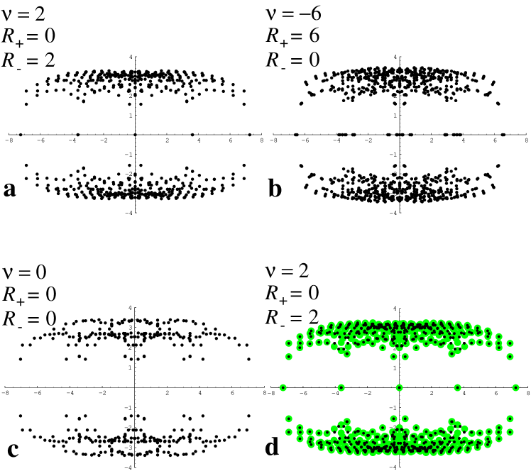
Figure 1: Plots of the spectra of $Q$ in the complex plane, for smooth background configurations (7) with $s=1,t=1$ (a), $s=1,t=-3$ (b), $s=1,t=0$ (c) and for $s=1,t=1$ (d). For Plots a, b, c all phases $\varphi_{\mu}$ were chosen to be zero, while for Plot d we have $\varphi_{\mu}=2\pi/7,\mu=1,2,3,4$ (small black dots) and compare it with the spectrum for the zero phase configuration (larger grey dots). $\nu$ is the topological charge of the gauge field used ($=2st$) and $R_{+},R_{-}$ are the numbers of real eigenvalues in the physical branch of the spectrum with positive and negative chirality.

Fig. 1.a shows the spectrum for the $s=1,t=1$ configuration, which has topological charge $\nu$ = 2. The first thing to note are the expected symmetries of the spectrum with respect to reflection at real and imaginary axis. All eigenvalues lie within a circle of radius 8 around the origin in the complex plane, as discussed in Section 2 and their imaginary parts are bounded by 4. The complex eigenvalues are well separated from the real axis, and many of them are degenerate (note that there are all together 2048 eigenvalues).

There are 32 real eigenvalues, all of them multiply degenerate. They lie in the vicinity of the values -8, -4, 0, 4, 8. We denote these branches where the real eigenvalues are found as $A^{*},B^{*},C,B,A$ as depicted in Fig. 2 and described in Table 1. As discussed in Section 2 Theorem, these branches correspond to the poles of the free propagator with periodic boundary conditions, situated at the corners of the Brillouin zone: $(0,0,0,0),(\pi,0,0,0)+3$ permutations, etc. For the $s=1,t=1$ configuration we find that the eigenvalues in the branches $A^{*},B^{*},C,B,A$ are degenerate and the branches are occupied by 2, 8, 12, 8 and 2 real eigenvalues. The pseudoscalar matrix elements $v^{\dagger}\;\Gamma_{5}v$ have the same sign for all eigenvalues within a branch, with the signs distributed among the branches as $-1,+1,-1,+1,-1$. All these features are as described in the lattice version (6) of the index theorem on the lattice and the right hand side terms of (6) for the principal branch are given by $R_{+}=0,R_{-}=2$.

Fig. 1.b and c show spectra for configurations with $s=1,t=-3$, having topological charge $\nu=-6$, and $s=1$ and $t=0$, with topological charge $\nu=0$. For the former case we find that the numbers of real eigenvalues in each branch have increased to 6, 24, 36, 24, 6. The signs of the pseudoscalar matrix elements are again equal for each branch, but now given by +1, -1, +1, -1, +1, since the topological charge is negative for this configuration. Thus $R_{+}=6,R_{-}=0$. For the spectrum in Fig. 1.c, which is for a configuration with zero topological charge, we find no real eigenvalue and $R_{+}=R_{-}=0$, compatible with (6).

Finally Fig. 1.d shows the spectrum for the s = 1, t = 1 case but now for all link variables we have chosen the non-zero value $\varphi_{\mu}=2\pi/7,\mu=1,2,3,4$ for the phase in (7) (small black dots in Fig. 1.d). The large grey dots indicate the spectrum for the configuration with zero phase. The figure nicely demonstrates, that the phase can shift several of the complex eigenvalues, but the real part of the spectrum, which reflects the topological charge (unchanged by the phase) remains invariant.

The general picture which emerges after our analysis of various spectra for smooth configurations (7) is summarized in Fig. 2 and Table 1. It entirely confirms formula (6).

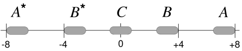
Figure 2: Schematic picture of the branches containing the real part of the spectrum of $Q$.

branch	$A^{*}$	$B^{*}$	$C$	$B$	$A$
$R_{-}-R_{+}$	$\nu$	$-4\nu$	$6\nu$	$-4\nu$	$\nu$
corners	$(\pi,\pi,\pi,\pi)$	$(\pi,\pi,\pi,0)$	$(\pi,\pi,0,0)$	$(\pi,0,0,0)$	$(0,0,0,0)$
of B.Z.		+ 3 perm.	+ 5 perm.	+ 3 perm.

Table 1: Properties of the branches containing the real part of the spectrum of $Q$.

4.2 Rough configurations

After testing the lattice version (6) of the index theorem for the smooth fields (7), we consider now the roughened fields (9). One expects, that for a small amount of roughening, which does not destroy the topological charge of the gauge field configuration, the relation (6) remains invariant.

Figure 3: Behavior of the spectrum of $Q$ (left-hand side plots) and the pseudoscalar matrix elements $v^{\dagger}\Gamma_{5}v$ plotted at the positions of the corresponding real eigenvalues (right-hand side plots) for the $s=1,t=1$ configuration when the roughening procedure (9) is applied. We show the results for roughening steps $n_{r}=2,6$ and 8, each with $\varepsilon=0.3$. For $n_{r}=2,6$ (upper four plots) the total number of real eigenvalues in the spectrum is $R_{+}^{all}+R_{-}^{all}$ = 32, according to (6), while for $n_{r}=8$ the gauge field becomes too rough, and (6) becomes violated giving rise to only 24 real eigenvalues in the spectrum.

In Fig. 3 we show the spectra of $Q$ (left-hand side plots) and the pseudoscalar matrix elements $v^{\dagger}\Gamma_{5}v$ plotted at the positions of the corresponding real eigenvalues (right-hand side plots) for the $s=1,t=1$ configuration having $\nu=2$. We show the results for roughening steps $n_{r}=2,6$ and 8, each step performed with $\varepsilon=0.3$ (see (9)). Comparing the spectra for the roughened configurations with the corresponding smooth spectrum Fig. 1.a, one finds that the degeneracy of the eigenvalues is lifted. For $n_{r}=2,6$ the real eigenvalues are still more or less concentrated in the branches $A^{*},B^{*},C,B,A$, but this structure becomes less pronounced with increasing number of roughening steps. For $n_{r}=2,6$ the total number of real eigenvalues is $R_{+}^{all}+R_{-}^{all}=32$ as expected from the index theorem ($=16\times|\nu|$). For $n_{r}=8$ the separation of the real spectrum into distinct branches has almost vanished, and the total number of real eigenvalues has dropped to $R_{+}^{all}+R_{-}^{all}=24$. Obviously the configuration becomes too rough and (6) does no longer hold. It is also interesting to note, that the complex part of the spectrum approaches the real line. This trend continues when $n_{r}$ is increased further, and the distribution of the eigenvalues becomes uniform inside the disk of radius 4 around the origin for random configurations (compare [10]). This observation nicely fits into the picture obtained from a strong coupling expansion. It can be shown, that the divergence of the pion propagator in strong coupling [37] is equivalent to a bound of 4 for the modulus of the eigenvalues of $Q$.

The plots for the pseudoscalar matrix elements on the right hand side of Fig. 3 confirm the obtained picture. For $n_{r}=2,6$ the matrix elements $v^{\dagger}Qv$ all have the same sign within the branches of the real spectrum. For $n_{r}=8$ some of the real eigenvalues, and thus their matrix elements have vanished, and the remaining matrix elements do no longer obey the sign pattern of the smoother configurations.

So far we presented only configurations where the matrix elements $v^{\dagger}\Gamma_{5}v$ have the same sign for all real eigenvalues in a branch of the spectrum. We found, that our test configurations (7), (9) also allow for cases where both signs occur within a branch. Due to the anti-periodic boundary conditions in time direction, configurations of the type $s=0,t\neq 0$, although they have $\nu=0$, give rise to spectra with an even number of real eigenvalues in each branch of the spectrum. Half of the corresponding eigenvectors have positive and half of them negative chirality and their contributions to the right hand side of (6) cancel. Fig. 4 shows the spectrum for the $s=0,t=-2$ configuration after 1 roughening step (left-hand side plot) and the corresponding pseudoscalar matrix elements $v^{\dagger}\Gamma_{5}v$ in all branches of the spectrum (right-hand side plot). Although the configuration has $\nu=0$ there are 12 real eigenvalues in the spectrum. The index theorem on the lattice (6) is nevertheless fulfilled, since the signs of the pseudoscalar matrix elements cancel in each branch of the spectrum.

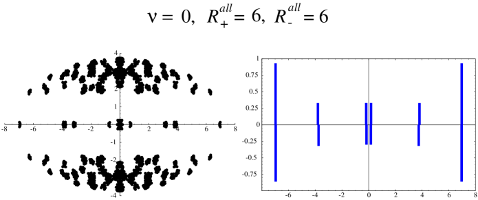
Figure 4: Spectrum of $Q$ (left-hand side plot) and the corresponding matrix elements $v^{\dagger}\Gamma_{5}v$ (right-hand side plot) for the $s=0,t=-2$ configuration after one step of roughening with $\varepsilon=0.3$. The gauge field has $\nu=0$ and according to formula (6), the sum of the signs of the matrix elements has to cancel for each branch of the spectrum. This feature is obvious from the right-hand side plot.

The left-hand side plot in Figure 4 also demonstrates nicely another important result of our analysis: The modulus of eigenvalues is no proper criterion to identify zero modes. From the spectrum plot in Fig. 4 it is obvious, that in the close vicinity of the real eigenvalues there cluster several complex eigenvalues. These complex eigenvalues have nothing to do with zero modes, since their pseudoscalar matrix elements vanish identically ($\sim 10^{-15}$ in our numerical analysis), while the matrix elements for the real eigenvalues are of order 1.

We remark, that increasing the size of one of the lattice sides to 6 does not affect the structure of the spectrum. For all sufficiently smooth configurations we analyzed, the lattice version (6) of the index theorem was confirmed, clearly demonstrating that the structure of the real eigenvalues is the part of the spectrum which remains invariant within the topological sectors.

4.3 Stability analysis for the topological features of the spectrum

In this section we present results from the analysis of the spectra for a whole sample of roughened gauge fields. This serves to demonstrate that the topological features of the spectrum are stable for a set of rough configurations (9) fluctuating around the smooth configurations (7).

In particular we analyzed the spectra for roughened gauge field configurations starting from the smooth configuration with $s=t=1(\nu=2)$. We then applied $n_{r}$ steps of the roughening procedure each with $\varepsilon=0.15$. For all together 15 values of $n_{r}$ in the range of $n_{r}=16$ to $n_{r}=38$ we computed spectra for 30 configurations at each $n_{r}$. For each sample of 30 spectra (at fixed $n_{r}$) we analyzed the topological features of the eigenvalues: The smooth configuration with $t=s=1$ has all together 32 real eigenvalues, distributed among the branches as $2,8,12,8,2$. The configuration has $\nu=2$, and thus according to (6) the quoted numbers are the minimal amount of real eigenvalues in each branch. In order to be compatible with (6) there is always the possibility that there are more real eigenvalues in a branch, but with different chirality of the corresponding eigenvectors, such that the difference of left- and right-handed contributions gives the numbers 2,8,12,8,2 for the branches. However, any spectrum with less than 32 real eigenvalues clearly violates (6). In almost all cases we analyzed, the breakdown of (6) was signalized by such a drop of the number of real eigenvalues below 32. For the following discussion we adopt as our criterion for a breakdown of (6) a violation of

$$\#\;of\;real\;eigenvalues\;\;=\;\;32\;.$$ (13)

We define the probability function $p(n_{r})$ to be the probability of finding (13) correct, and compute it for each sample of 30 spectra at fixed $n_{r}$. Fig. 5 shows the probability $p(n_{r})$ (circles, scale on the left vertical axis) for different values of $n_{r}$. In the figure we also display the average value of the gauge field action per plaquette $\overline{S}$ (diamonds, right vertical scale).

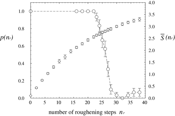
Figure 5: Probability $p$ of finding (6) correct (circles, left vertical scale) as a function of the number of roughening steps $n_{r}$, each with $\varepsilon=0.15$. We also show the average value of the gauge field action per plaquette $\overline{S}$ (diamonds, right vertical scale).

The figure shows nicely, that there is a rather large number of roughening steps where the topological structure of the spectrum remains unperturbed, i.e. $p=1$ (from $n_{r}=0$ to $n_{r}=22$). During these roughening steps the action per plaquette $\overline{S}$ increases (starting with a value of 0.1 at $n_{r}=0$) roughly by a factor of 25 which demonstrates the stability of the topological structure in more physical units. Then after 22 roughening steps the probability $p$ for the index theorem (6) to hold drops sharply reaching a level of $p\sim 0.05$ at $n_{r}=30$. Under further roughening the probability function keeps fluctuating around this value. The plot nicely demonstrates the stability of the topological structure of the spectrum. In particular real eigenvalues and the pseudoscalar matrix elements of their eigenvectors are seen to be rather stable which underlines their topological nature.

We performed the same analysis (with less statistics) for roughened gauge fields starting from the smooth $t=s=2$ configuration. Again we observed a large region where the topological structure of the spectrum remained stable, with a rather sharp drop of the probability function at the end of the region. We found that this drop was at a different value of the action per plaquette (approximately 25 % smaller), indicating that, at least for the lattice size we considered, there is no universal threshold in terms of the action where a topological sector gets destroyed.

5 Discussion of the overall picture in the fully quantized theory using QED₂ as an example

In the last section we have numerically investigated the form (6) of the index theorem on the lattice using test configurations for 4-D SU(2) lattice gauge theory. The set of gauge field configurations (7), (9) we used is of course rather restricted. On the other hand, testing the obtained picture in a simulation of QCD₄ is certainly too demanding for present computer technology. However it is possible [25] to analyze the Atiyah-Singer index theorem (6) in the simpler model of QED₂.

QED₂ is not only considerably cheaper to simulate, but also has a very simple expression [38] for its topological charge: $\nu[U]\;=\;\frac{1}{2\pi}\sum_{x}\theta_{p}(x)$, where $\theta_{p}(x)=-i\ln U_{12}(x)$ with $\theta_{p}(x)\in(-\pi,\pi)$. Configurations where $U_{12}(x)=-1$ for one of the plaquettes are so-called exceptional configurations [29], and no topological charge can be assigned to them. They are of measure zero in the path integral.

Again it is possible to use the Atiyah-Singer index theorem in the continuum as a guiding line of what to expect on the lattice. For QED₂ there holds another index theorem, sometimes referred to as Vanishing Theorem [39]. It states that there are either only left- or only right-handed zero modes. Furthermore, taking into account that in $D=2$ there are 4 species of fermions, 1 in the physical branch and 3 doublers, one expects to find

$$\#\;of\;real\;eigenvalues\;=\;4\Big{|}\nu[U]\Big{|}\;.$$ (14)

We define $p$ to be the probability of finding (14) correct and evaluate this probability for a whole ensemble of Monte Carlo configurations generated in a simulation of QED₂ with dynamical fermions [25]. We computed $p$ for several values of $L=T$ and $\beta$. The hopping parameter $\kappa$ was always chosen close to the critical value for the given $L$ and $\beta$. In Fig. 6 we plot the probability function $p$ as a function of the dimensionless ratio $\beta/L^{2}$.

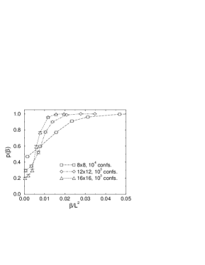
Figure 6: Probability $p$ of finding (14) correct as a function of $\beta/L^{2}$. We show our results for lattice sizes $L=8,12$ and 16. The symbols are connected to guide the eye.

It is obvious from this plot that when sending $L\rightarrow\infty$ and holding $\beta/L^{2}$ fixed (which corresponds to sending $L\rightarrow\infty$ while holding $\xi/L$ fixed), the probability function $p$ approaches 1. This implies that (14) holds with probability 1 in the continuum limit. A detailed analysis [25] shows, that this result is essentially uniform in $\nu$ and also the chiral properties of the eigenvectors are conform with the expectations from Atiyah-Singer Index Theorem and Vanishing Theorem.

It has to be stressed, that this result is not restricted to some subset of configurations (as is our analysis for QCD₄) since it was established using the complete set of Monte-Carlo configurations. This demonstrates that the lattice version of the index theorem holds in fully quantized QED₂. We remark, that in [14] the interplay between the topological charge and the spectrum of the lattice Dirac operator was further investigated by demonstrating within the overlap formalism that the chiral condensate in the Schwinger model originates from the sectors with topological charge $\pm 1$.

6 Summary and outlook

The fact that for the Wilson-Dirac operator hermitian conjugation can be implemented as a similarity transformation with $\gamma_{5}$ has an important implication for the chiral properties of the eigenvectors of the fermion matrix: Only eigenvectors with real eigenvalues have non-vanishing pseudoscalar matrix-elements and thus should be interpreted as the lattice equivalents of the continuum zero-modes. The lattice version of the Atiyah-Singer index theorem thus connects the topological charge of the spectrum to the number of real eigenvalues.

In this contribution we analyzed those features of the spectrum of the Wilson-Dirac operator that are connected to non-trivial topology of the gauge field. In particular we demonstrated the stability of the real eigenvalues and their corresponding pseudoscalar matrix elements under adding fluctuations to the gauge fields. This shows the topological nature of the real part of the spectrum. For the computationally less demanding case of U(1) gauge fields in two dimensions we analyzed the lattice index theorem for a complete set of configurations from a simulation with dynamical fermions. It was shown, that the $\beta\rightarrow\infty$ limit is dominated by configurations where the lattice index theorem holds with probability one.

The next logical step in a numerical analysis of the lattice index theorem would be to test the four-dimensional Wilson-Dirac operator with gauge field configurations from a Monte Carlo ensemble generated in a quenched or even unquenched simulation. On the analytic side it would be interesting to investigate the role of the topological part of the spectrum in fermionic correlation functions. In particular in a spectral decomposition of fermionic $n$-point functions one could try to separate the part corresponding to eigenvectors with real eigenvalues. The lattice index theorem (6) shows that these contributions are intimately connected to the topological sector of the background gauge field. Interesting insights into U(1) problem and Witten-Veneziano type formulas could be obtained.

Acknowledgment: We thank Christian B. Lang for valuable discussions during the course of this work.

Note added in the revised version: In the meantime five more contributions related to our work appeared as preprints. In [40] further studies of the spectral flow of the overlap hamiltonian are performed. In particular instanton configurations and gauge fields from unquenched simulations are considered. Furthermore the effect of an $O(a)$-improving clover term is discussed. [41] also analyzes the effect of the clover term on the level crossings for the overlap hamiltonian. Improvement seems to be a viable method to enhance the chiral properties of the eigenstates. In [42] the spectrum of the un-modified Wilson-Dirac operator is analyzed in the Schwinger model and perturbative arguments for the stability of the real eigenvalues are given. Finally in [43] the spectrum of the fixed point lattice Dirac operator in the Schwinger model is studied.

References

- [1]
- [2] M. Atiyah and I.M. Singer, Ann. Math. 87 (1968) 596; Ann. Math. 93 (1971) 139.
-
[3]
P. Colella and O.E. Lanford III, in: Constructive Quantum Field Theory (Erice 73),
G. Velo and A. Wightman (Eds.), Springer Lecture Notes in Physics,
Springer 1973, New York;
J. Glimm and A. Jaffe, Quantum Physics, Springer 1987, New York;
A. Ashtekar, J. Lewandowski, D. Marolf, J. Mourao and T. Thiemann, in: Geometry of Constrained Dynamical Systems, Cambridge 1994 (preprint hep-th/9408108). - [4] B. Alles, M.D. Elia, A. Di Giacomo and R. Kirchner, preprint hep-lat/9711026.
- [5] F. Karsch, E. Seiler and I.O. Stamatescu, Nucl. Phys. B271 (1986) 349.
- [6] J. Smit and J.C. Vink, Nucl. Phys. B286 (1987) 485.
-
[7]
J. Smit and J.C. Vink,
Phys. Lett.
194B (1987) 433;
M.L. Laursen, J. Smit and J.C. Vink, Nucl. Phys. B343 (1990) 522. - [8] Nucl. Phys. B284 (1987) 234; Nucl. Phys. B298 (1988) 557.
-
[9]
J. Smit and J.C. Vink,
Nucl. Phys.
B303 (1988) 36;
J.C. Vink, Nucl. Phys. B307 (1988) 549. - [10] R. Setoodeh, C.T.H. Davies and I.M. Barbour, Phys. Lett. 213B (1988) 195.
- [11] S. Itoh, Y. Iwasaki and T. Yoshié, Phys. Rev. D36 (1987) 527; Phys. Lett. 184B (1987) 375.
- [12] R. Narayanan and H. Neuberger, Phys. Rev. Lett. 71 (1993) 3251; Nucl. Phys. B412 (1994) 574; Nucl. Phys. B443 (1995) 305.
- [13] R. Narayanan and H. Neuberger, Phys. Lett. B348 (1995) 549.
- [14] R. Narayanan, H. Neuberger and P. Vranas, Phys. Lett. B353 (1995) 507.
- [15] R. Narayanan and P. Vranas, Nucl. Phys. B506 (1997) 373.
-
[16]
R. Narayanan and R.L. Singleton Jr.,
Nucl. Phys. Proc. Supl.
63 (1998) 555;
R.G. Edwards, U.M. Heller, R. Narayanan and R.L. Singleton Jr., Nucl. Phys. B518 (1998) 319. - [17] T. Kalkreuter, Phys. Rev. D51 (1995) 1305; Nucl. Phys. B (Proc. Supl.) 49 (1996) 168.
- [18] T. Kalkreuter and H. Simma, Comput. Phys. Commun. 95 (1996) 1.
-
[19]
M.A. Halasz, T. Kalkreuter and J.J.M. Verbaarschot,
Nucl. Phys. B (Proc. Supl.)
53 (1997) 266;
M.E. Berbenni-Bitsch, S. Meyer, A. Schäfer, J.J.M. Verbaarschot and T. Wettig, Phys. Rev. Lett. 80 (1998) 1146. - [20] W. Bardeen, A. Duncan, E. Eichten and H. Thacker, Phys. Rev. D57 (1998) 1633; Phys. Rev. D57 (1998) 3890.
-
[21]
J.W. Negele,
preprint hep-lat/9709129;
T.L. Ivanenko and J.W. Negele, Nucl. Phys. Proc. Suppl. 63 (1998) 504. - [22] J.B. Kogut, J.-F. Lagaë and D.K. Sinclair, Nucl. Phys. Proc. Suppl. 63 (1998) 433.
- [23] L. Venkataraman and G. Kilcup, Nucl. Phys. Proc. Suppl. 63 (1998) 826.
- [24] M. García Pérez, A. Gonzalez-Arroyo, A. Montero and C. Pena, Nucl. Phys. Proc. Suppl. 63 (1998) 501.
- [25] C.R. Gattringer, I. Hip and C.B. Lang, Nucl. Phys. B508 (1997) 329; Nucl. Phys. Proc. Suppl. 63 (1998) 498.
-
[26]
K. Jansen, C. Liu, H. Simma and D. Smith,
Nucl. Phys. B (Proc. Supl.)
53 (1997) 262;
D. Smith, H. Simma and M. Teper, Nucl. Phys. Proc. Suppl. 63 (1998) 558. - [27] I. Montvay and G. Münster, Quantum Fields on a Lattice, Cambridge University Press 1994, Cambridge.
- [28] D.H. Weingarten and J.L. Challifour, Ann. Phys. 123 (1979) 61.
- [29] M. Lüscher, Commun. Math. Phys. 85 (1982) 39.
- [30] A. Phillips and D. Stone, Commun. Math. Phys. 103 (1986) 599.
- [31] I. Fox, J. Gilchrist, J. Laursen and G. Schierholz, Phys. Rev. Lett. 54 (1985) 749.
-
[32]
P. de Forcrand, M. García Pérez and I.-O. Stamatescu,
Nucl. Phys.
B499 (1997) 409;
P. de Forcrand, M. García Pérez, J.E. Hetrick and I.O. Stamatescu, Nucl. Phys. Proc. Suppl. 63 (1998) 549. - [33] T. DeGrand, A. Hasenfratz and T. Kovacs, Nucl. Phys. B505 (1997) 417; Nucl. Phys. Proc. Suppl. 63 (1998) 528; Nucl. Phys. B520 (1998) 301.
- [34] C.R. Gattringer, I. Hip and C.B. Lang, Phys. Lett. B 409 (1997) 371.
- [35] J. K. Cullum and R. A. Willoughby, Lanczos algorithms for large symmetric eigenvalue computations, Vol. 1. Theory, Birkhäuser, Boston, 1985.
- [36] I. Barbour, E. Laermann, Th. Lippert and K. Schilling, Phys. Rev. D46 (1992) 3618.
- [37] K.G. Wilson, in: New Phenomena in Subnuclear Physics (Erice 75), A. Zichichi (Ed.), Plenum 1977, New York.
-
[38]
R. Flume and D. Wyler,
Phys. Lett.
108B (1981) 317;
C. Panagiotakopoulos, Nucl. Phys. B251 (1985) 61;
A. Phillips, Ann. Phys. 161 (1985) 399;
M. Göckeler, A.S. Kronfeld, G. Schierholz and U.-J. Wiese, Nucl. Phys. B404 (1993) 839;
H. Gausterer and M. Sammer, preprint hep-lat/9609032. -
[39]
J. Kiskis,
Phys. Rev.
D15 (1977) 2329;
N.K. Nielsen, B. Schroer, Nucl. Phys. B127 (1977) 493;
M.M. Ansourian, Phys. Lett. 70B (1977) 301. - [40] R.G. Edwards, U.M. Heller and R. Narayanan, Nucl. Phys. B522 (1998) 285; preprint hep-lat/9802016.
- [41] H. Simma and D. Smith, preprint hep-lat/9801025.
- [42] P. Hernandez, preprint hep-lat/9801035.
- [43] F. Farchioni and V. Laliena, preprint hep-lat/9802009.