Phase Structure of Dynamical Triangulation Models in Three Dimensions

Abstract

The dynamical triangulation model of three–dimensional quantum gravity is shown to have a line of transitions in an expanded phase diagram which includes a coupling $\mu$ to the order of the vertices. Monte Carlo renormalization group and finite size scaling techniques are used to locate and characterize this line. Our results indicate that for $\mu<\mu_{1}\sim-1.0$ the model is always in a crumpled phase independent of the value of the curvature coupling. For $\mu<0$ the results are in agreement with an approximate mean field treatment. We find evidence that this line corresponds to first order transitions extending to positive $\mu$. However the behavior appears to change for $\mu>\mu_{2}\sim 2.0-4.0$. The simplest scenario that is consistent with the data is the existence of a critical end point.

PACS numbers: 04.60.+n, 05.70.Jk, 11.10.Gh

I Dynamical Triangulations with a Measure Term

Triangulations provide a discretization of curved Euclidean spacetimes. In the Regge approach, a specific simplicial lattice is chosen a priori and the properties of the spacetime are determined by the length of the lattice links. A complementary approach, dynamical triangulations, fixes the length of the links to an invariant cut-off and allows the lattice connectivity to determine the geometry of the spacetime. This paper uses the latter approach. A lattice representation of the Einstein-Hilbert action is

$$S=\alpha N_{0}-\beta N_{D}$$ (1)

where $N_{0}$ is the number of vertices and $N_{D}$ the number of simplices in the triangulation (the latter is then also the volume), D is the dimension of the system and $\alpha$ and $\beta$ are corresponding chemical potentials. The coupling $\beta$ serves as the cosmological constant while $\alpha$ is related to Newton’s gravitational constant. The connectivity of a triangulation plays the same role as the metric in continuous manifolds in the sense that points joined by a link are considered close together while those not connected are considered further apart. Continuum theories of quantum gravity generally involve an integration over all possible physically inequivalent metrics. In dynamical triangulation models, a sum over triangulations (i.e a sum over all allowed connectivities) fulfills the same need. Consequently, the partition function for the dynamical triangulation model of quantum gravity is

$$Z=\sum_{T}\rho\left(T\right)e^{S}$$ (2)

where the sum is over all possible triangulations with fixed topology, $S$ is the action given above and the term $\rho(T)$ allows for the possibility of a non-trivial measure in the space of triangulations. Matter can be coupled to the gravity by adding appropriate terms to eqn. (1) and including a sum over the matter degrees of freedom in eqn. (2).

These models of quantum gravity have proven themselves in two dimensions where analytical results are available both in the continuum and on the lattice. They agree in all cases where comparisons are possible. This agreement occurs with trivial measure $\rho(T)=1$. In higher dimensions, it may be necessary to utilize a non-trivial measure term in order to obtain an acceptable lattice theory. In this paper, the three–dimensional model is modified so as to include such a measure term. The resulting phase diagram is studied in detail.

There is additional motivation for adding a measure term. As in lattice gauge theories, it is expected that dynamical triangulation models must have a second order phase transition in their phase diagram if they are to have a continuum limit and therefore a chance at physical relevance. Many two–dimensional models have the necessary continuous transition. However, in three dimensions, while the simple action of eqn. (1) does have a phase transition, it is first order. The phase diagram is one–dimensional (parameterized by $\alpha$) since $\beta$ is used to fix the volume. Thus, it is natural to expand the phase diagram by including some new coupling so that there is a larger territory in which to search for continuous phase transitions. Expanded phase diagrams have been examined in the past, produced by adding both spin matter [1] and gauge matter [2] to the system, but no second order phase transition was found. Modifying the action $S$ to include a suitable measure term can be viewed as another attempt to expand the phase diagram so as to produce a continuous phase transition. The expectation is that the transition point $\alpha_{t}$ at $\mu=0$ will extend into a transition line $\alpha_{t}\left(\mu\right)$ in the $(\alpha,\mu)$ plane.

In [3] a lattice version of a family of measures $\rho(T)$ is introduced by adding a new term to the action

$$S=\alpha N_{0}-\beta N_{D}+\mu M$$ (3)

where

$$M=\sum_{i\in N_{0}}\ln\left({O_{i}\over{D+1}}\right)$$ (4)

and $O_{i}$ is the number of $D$-simplices which include the vertex $i$, commonly referred to as the “order” of $i$. This additional term in the action corresponds to a continuum measure of the form

$$\prod_{x}g^{\mu/2}$$ (5)

($g$ being the determinant of the metric). In two dimensions, it is known from Monte Carlo renormalization group [4] and exact calculations [5] that any lattice theory with $\mu>0$ yields the same continuum limit: this new term behaves as an irrelevant operator in the renormalization group sense. In higher dimensions, it is not known whether the operator changes the fixed point structure of the theory and if so, how the bare $\mu$ should be chosen to approach a non-trivial continuum limit. These are the questions we attempt to address here for the case $D=3$.

II Computational Techniques

We have used Monte Carlo simulations to do computations based on eqn. (3). Three techniques have been most useful in analyzing the simulations and drawing conclusions from them: the renormalization group approach, finite size scaling, and histograms of the time series data.

The renormalization group has proven to be a powerful technique for understanding field theory and statistical mechanics in flat space. When combined with Monte Carlo simulation it allows a non-perturbative determination of the flows and phase structure. A formulation of the renormalization group applicable to dynamical triangulations has been developed and established in previous papers[6, 4, 7, 8]. It is useful to recall some details of this scheme. One iteration of the renormalization group transformation eliminates a single vertex from the lattice. This transformation is iterated until the number of vertices in the blocked system is reduced to a target number. Two operators are used to monitor the flow in the expectation values: $<N_{3}>$ and $<M>$. Their values after blocking depend both on the initial volume of the system and the bare couplings. The latter may be used to label different flow lines while the former parametrizes distance along such a flow line. For $\mu\leq 0$, as the renormalization group transformation is iterated, all flows initially head toward a common area in the $(N_{3},M)$ plane. Eventually, as the iterations continue, the flows diverge and head in directions determined by the phase the couplings correspond to. For large positive $\mu$, the flows diverge immediately.

The renormalization group scheme has been tested previously (in three dimensions) only near the transition $\alpha=\alpha_{t}\left(\mu\right)$ for $\mu=0$. It is important to have an independent means of checking whether or not the renormalization group prediction of flows, transition couplings, and transition orders is actually correct for $\mu\neq 0$. If consistent, these independent means serve to strengthen the case provided by the renormalization group. Vertex susceptibilities $\chi$ provide just such a check.

$$\chi=(<N_{0}^{2}>-<N_{0}>^{2})/N_{3}$$ (6)

Close to a phase transition this quantity will typically exhibit a peak. The position of this peak is called the pseudocritical coupling. In the infinite volume limit this pseudocritical coupling converges to the true transition coupling. The difference between this transition coupling and the pseudocritical coupling is one measure of the magnitude of finite size effects. The scaling of the height of the peak in $\chi$ with system volume can be used to extract a scaling exponent $\omega$. A value for $\omega$ of unity would indicate a first order transition. Smaller values are consistent with continuous critical behavior.

If a first order transition is strong enough, it can be seen in the Monte Carlo time series. A double peak structure in a histogram of the vertex number data is a classic sign of a first order phase transition. Continuous transitions possess only a single peak in this histogram.

For fixed values of $\mu$, we search for a transition as a function of $\alpha$ using the above techniques. A variety of values of $\mu$ are considered, including both positive and negative values. All runs are for (quasi) fixed volumes $N_{3}$ in the range of $4000$ to $16000$. Typically ten million sweeps were performed where one sweep is defined as $N_{3}$ attempted elementary moves. For values of $\mu\sim 4$, ten million was found to be much too small a number of sweeps.

III Results for the Transition Line

A $\mu=0$.

The transition is known to be strongly first order for $\mu=0$. This is illustrated in fig. 1 which shows a Monte Carlo time series for the vertex number $N_{0}$ and in fig. 2 which displays a histogram of the same data. The plots show clearly the existence of two metastable states connected by tunneling events typical of a discontinuous phase transition. This observation is in agreement with earlier studies [9]. On one side of the transition the system is in a crumpled phase and on the other side it is in a branched polymer phase. The crumpled phase is characterized by a vertex density $<N_{0}>/N_{3}$ which goes to zero as the volume $N_{3}$ gets large. In the branched polymer phase this ratio approaches $1/3$.

FIG. 1.: Time history of the number of vertices during a simulation at $\mu=0$, $\alpha=4.0$, and $N_{3}=8000$. Time is in units of $1000N_{3}$ attempted updates.

FIG. 2.: A histogram of the data presented in fig. 1.

The vertex susceptibility also reveals the first order nature of the transition: in fig.3 results from a system with $8000$ simplices (plotted as circles) clearly display a huge peak. The error bar at the peak is so large because there are relatively infrequent tunnelings between metastable states at the transition. Notice that there is a roughly constant characteristic value of the susceptibility in the crumpled phase (small $\alpha$) and a much smaller roughly constant characteristic value in the branched polymer phase (large $\alpha$). These features will be visible at other values of $\mu$ as well. The arrows denote the range of critical coupling determined from a study of the renormalization group flows (computed previously [6] and not reproduced here). Notice that it is consistent with the position of the peak in $\chi$. This is an indication that finite size effects for $N_{3}=8000$ are small at $\mu=0$.

However data from a system with $4000$ simplices (with plus as the plotting symbol) is included in the plot for comparison. (The error bars are roughly the size of the plotting symbols and were left off for aesthetic purposes). The peak is not nearly as high for the smaller system. For significantly smaller systems the peak would become indistinguishable from the background. Furthermore, it is clear that the pseudocritical coupling is very far from the true critical coupling for this lattice size implying that finite size effects are large. The moral to be drawn from this is that it would be very hard to infer the transition order correctly from lattices which are too small.

FIG. 3.: Vertex susceptibility as a function of $\alpha$ for $\mu=0.0$. Arrows indicate the renormalization group prediction for the transition region.

B $\mu=-0.50$.

For $\mu\neq 0$ the transition value of $\alpha$ has typically not been previously determined (however, see recent work in [10]). The renormalization group flows provide a convenient method of searching for the transition since the flows eventual diverge, flowing toward small node density in the crumpled phase and large node density in the branched polymer phase. Fig. 4 illustrates this with several values of $\alpha$ chosen to be near the transition. Flows similar to the case of $\mu=0$ are seen here. Each line represents a different value of $\alpha$ and motion along that line (up and to the right) represents the evolution of the volume $N_{3}$ and the average of $M$ as the initial volume is increased. Since the renormalization group is iterated until the number of vertices in the blocked system is the same as the number of vertices in the original system when the original volume is $500$, systems with larger initial volumes require more vertex deletions. Hence, motion along the line corresponds to expectation values for effective theories at larger and larger length scales. The values of $\alpha$ are, reading from right to left in the figure, 4.7, 4.8, 4.9, and 5.0. The rightmost line, which continues out of the boundaries of the plot, moves toward larger volumes. Since the vertex number is fixed this means the vertex density is heading toward zero. This is characteristic of the crumpled phase. The leftmost lines cannot go left indefinitely because there is a lower bound on the volume given a number of vertices. These leftmost flows correspond to the branched polymer phase. One flow ends up moving neither right nor left. The coupling for this flow is presumably near the transition value. Further points along the flow (i.e. larger volumes) are needed to determine which phase it is in or whether it approaches a fixed point.

FIG. 4.: Renormalization group flows with $\mu=-0.50$.

At a strongly first order transition, such as in three dimensions with $\mu=0$, it is not necessary to go to large volumes to see what the phase is, so there are no intermediate flows [8]. In four dimensions, the corresponding transition appears second order at small volumes, and there are intermediate flows similar to the one in the figure. At larger volumes, there is now evidence that this latter transition is actually first order [11]. Thus the three–dimensional models at (moderate) negative $\mu$ seem to behave somewhat similarly to the the four–dimensional theory at $\mu=0$. We might expect them to display large finite size effects and this is verified below: it is necessary to go to large volumes to get the pseudocritical couplings determined from vertex susceptibilities to agree with the renormalization group predictions.

Fig. 5 shows the time history for a simulation at the transition and fig. 6 is a histogram of that data. The existence of two metastable states as revealed in these plots lends support to the idea that the transition remains first order as $\mu$ is varied towards negative values.

FIG. 5.: Time history of the number of vertices during a simulation at $\mu=-0.50$, $\alpha=4.85$, and $N_{3}=16000$. Time is in units of $1000N_{3}$ attempted updates.

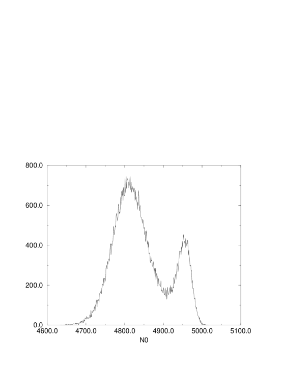
FIG. 6.: A histogram of the data presented in fig. 5.

The vertex susceptibility is shown in fig. 7 There are plateaus of characteristic values in both the crumpled and the branched polymer phases. This time, for $N_{3}=8000$ (with circles as the plotting symbol), the plateaus are separated by a much smaller peak. This peak is noticeably to the left of the range of transition values suggested by the renormalization group flows (obtained with maximum volume $N_{3}=8000$). Data for $N_{3}=16000$ (with squares as the plotting symbol) show that the transition is moving toward greater $\alpha$ as the volume increases. This is more consistent with the renormalization group result. This large change in the pseudocritical coupling is indicative of the presence of large finite volume corrections. The large error bar on the peak for $N_{3}=16000$ is again due to the presence of just a few fluctuations between metastable states.

FIG. 7.: Vertex susceptibility as a function of $\alpha$ for $\mu=-0.50$. Arrows indicate the renormalization group prediction for the transition region.

C $\mu=-0.75$.

For the limited lattice sizes used in this study the situation becomes somewhat unclear at large negative coupling. For moderate lattice volumes there are no clear signals of metastability and a histogram of the vertex number shows no strong double peak structure. One might argue that the explanation is that the latent heat is small in this regime – perhaps going to zero for some critical $\mu$ [10]. However, as we have shown our data indicate that finite size effects get progressively larger for increasing negative $\mu$. These finite size effects can obscure the true critical behavior – on small to moderate lattice sizes the first order transition can appear continuous or even absent. Indeed if we assume the correct order parameter for the transition is $<N_{0}/N_{3}>$ and if we assume this vanishes in the crumpled phase (supported by the mean field arguments we present later) then the observed latent heat is increasing as $\mu$ is made more negative. This would seem to argue against a critical end point for $\mu<0$.

Further evidence supporting this scenario is presented in fig. 8 which shows the vertex susceptibility for $\mu=-0.75$. For $8000$ simplices (circles), the peak has completely vanished and is replaced with a gradual interpolation between the two characteristic values. The range of transition values indicated by the renormalization group is now even further to the right of the crossover region in the susceptibilities which is an indication that finite size effects are even larger here than for $\mu=-0.50$. The data for $16000$ simplices (squares) shows the beginnings of a peak closer to the critical regime predicted by the renormalization group method (which used a maximum of 8000 simplices). It appears that finite size effects dominate the physics even at this large volume and an even larger volume would be necessary to extract unambiguous results. We have not attempted such a simulation.

FIG. 8.: Vertex susceptibility as a function of $\alpha$ for $\mu=-0.75$. Arrows indicate the renormalization group prediction for the transition region.

D $\mu=2.0$.

We have argued that the data favor a first order line for $\mu<0$. Our evidence concerning the $\mu$ dependence of finite size effects suggests that simulations for $\mu>0$ may suffer smaller finite size effects. This is indeed seen: for $1.0<\mu<2.0$ it becomes possible to see tunneling between metastable states on smaller lattices ($N_{3}=4000$). A time history for $\mu=2$ and $N_{3}=4000$ is given in fig. 9 and the corresponding histogram is given in fig. 10. Similar results are obtained at $\mu=1$. Analysis of the vertex susceptibility and renormalization group flows also show strong support for a first order phase transition at these points on the phase boundary.

FIG. 9.: Time history of the number of vertices during a simulation at $\mu=2$ and $N_{3}=4000$.

FIG. 10.: A histogram of the data presented in fig. 9.

E $\mu=4.0$.

For $\mu=4$, results are quite different. The renormalization group flows are shown in fig.11. A dashed line has been included in the plot as a reminder that the flows all start at $N_{3}=500$. Here the flows diverge immediately rather than briefly traveling identical paths as they did for $\mu\leq 0$. The flows fan out more uniformly across the plane.

FIG. 11.: Renormalization group flows with $\mu=4.0$.

Examining the vertex susceptibility (fig. 12) reveals that there is still a peak but that it fails to scale with volume. There are no signs of metastability for any value of $\alpha$. There are also no indications of large finite size effects, so the data suggest that there is no transition at this value of $\mu$. Perhaps the first order line terminates for a value of $\mu$ between $2$ and $4$. One other significant feature of the simulations is that there the observed autocorrelation times become extremely long. These autocorrelation times could be due to the presence of a nearby critical end point. It is also possible that for this value $\mu$ we have entered a new phase which is exceptionally difficult to simulate.

FIG. 12.: Vertex susceptibility for $\mu=4.0$

F Summary

The above results as well as some data for other values of $\mu$ provide the basis for a plot of the transition through the $(\alpha,\mu)$ plane. The results are displayed in fig. 13. The error bars in the figure change direction at $\alpha=9$ because for smaller values of $\alpha$ it is convenient to fix $\mu$ and vary $\alpha$ when searching for the phase boundary while for larger values of $\alpha$ it is more convenient to fix $\alpha$ and vary $\mu$. Notice that the transition appears to head off to large values of $\alpha$ as $\mu$ is decreased further than $\mu\sim-1$. Indeed our data is consistent with a curve which asymptotes to a horizontal line. Thus it appears that there is a value of $\mu$ below which there is no phase transition as a function of $\alpha$: there is only a crumpled phase. This is because the transition line becomes horizontal. Our results suggest that the transition is first order for $\mu<=2$ with the first order line ending for $\mu$ somewhere between $2$ and $4$. The dotted curve is the prediction of our mean field treatment which will be discussed in the following section.

FIG. 13.: Phase diagram of three–dimensional triangulations with measure term.

IV Mean Field Arguments

In a previous paper [12] we have discussed how the two phases of the dynamical triangulation models can be understood in terms of a condensation of singular vertices. In general the crumpled phase in $D$ dimensions consists of a single $(D-3)$-simplex common to a number of $D$-simplices which diverges as a power of the total volume. As the vertex coupling $\alpha$ is increased this structure becomes unstable disappearing entirely in the branched polymer phase. The transition is driven by the fluctuations in this singular structure [13].

With this as a motivation we have considered an ansatz for the partition function which replaces the counting of distinct triangulations with the problem of enumerating the possible orders of the vertices.

$$Z\left(N_{0},N_{3}\right)=\sum_{n_{i}}\prod_{i=1}^{N_{0}}\omega\left(n_{i}\right)\delta\left(\sum_{i=1}^{N_{0}}n_{i}-cN_{3}\right)$$ (7)

The factors $\omega\left(n_{i}\right)$ give the probability that the vertex $i$ has order $n_{i}$ and the final $\delta$-function constraint reflects the fact that the total order is proportional to the total volume Notice that this approach is based on two approximations; that the counting of states can be done by counting vertex orders and that the latter can be done in a mean field manner by assuming that each varies independently of the others except for the global constraint. Such a model describes well certain branched polymer models [14] and has been proposed as relevant to the description of dynamical triangulations [15]. This general constrained mean field model was solved in [17] for general probabilities $\omega\left(n_{i}\right)$. As discussed in [12], for describing dynamical triangulations the factors of $\omega\left(n_{i}\right)$ should be taken to be the number of triangulations of the $2$-sphere (in three dimensions) surrounding a given vertex $i$. We take the form [16]

$$\omega\left(n_{i}\right)=\left(\frac{n_{i}}{4}\right)^{-7/2}\exp{\beta_{2}^{c}\left(n_{i}-4\right)}$$ (8)

This has the correct asymptotics ($\beta_{2}^{c}=\ln{\frac{16}{3\sqrt{3}}}$) and yields unity for the minimal triangulation of the $2$-sphere with $4$ simplices. Notice that it is now trivial to incorporate the effects of the measure term – the power is simply modified from $-7/2$ to $-7/2+\mu$. Using the results of [17] one can write the partition function of this model in the thermodynamic limit as

$$Z=\frac{1}{2\pi}\exp{\left(\left(-\log{\lambda}+\beta_{2}^{c}\right)cN_{3}+\ln{F_{\mu}\left(\lambda\right)}N_{0}\right)}$$ (9)

where the parameter $\lambda$ is the solution of the equation ($\rho=N_{0}/N_{3}$)

$$\frac{c}{\rho}=\frac{\lambda F^{\prime}_{\mu}\left(\lambda\right)}{F_{\mu}\left(\lambda\right)}$$ (10)

and, here

$$F_{\mu}\left(\lambda\right)=\frac{4^{7/2}}{\exp{4\beta_{2}^{c}}}\sum_{q=2}^{\infty}\left(2q\right)^{-7/2+\mu}\lambda^{2q}.$$ (11)

This model exhibits two phases; for $\rho<\rho_{c}=c\frac{F\left(1\right)}{F^{\prime}\left(1\right)}$ the parameter $\lambda=1$ and the system is in a collapsed phase where vertices of small order behave independently and the global constraint is satisfied by a small number of vertices which are shared by a number of simplices on the order of the volume. This regime is identified with the crumpled phase of the dynamical triangulation model. Conversely for $\rho>\rho_{c}$ the parameter $\lambda$ varies between zero and one and the free energy varies continuously with $\rho$. The distribution of vertex orders then behaves as

$$p\left(n\right)\sim\omega\left(n\right)e^{-n\log{\lambda}}$$ (12)

This phase is then identified with the branched polymer phase in the dynamical triangulation model. As $\rho$ (and hence $N_{0}$) is varied (by varying the coupling $\alpha$) the system moves between these two phases. In practice a canonical ensemble in which the vertex number can fluctuate is used.

$$Z_{C}=\sum_{N_{0}}e^{\alpha N_{0}}Z\left(N_{0},N_{3}\right)$$ (13)

The phase diagram then contains two phases corresponding to the crumpled and branched polymer phase separated by a first order phase transition [18]. In the branched polymer phase $N_{0}/N_{3}$ varies continuously with $\alpha$ tending to $\rho_{c}$ as $\alpha-\alpha_{t}\left(\mu\right)\to 0^{+}$. Conversely, $N_{0}/N_{3}\to 0$ in the crumpled phase $\alpha<\alpha_{t}\left(\mu\right)$. The phase boundary is predicted to be

$$\alpha_{t}\left(\mu\right)=-\log{F_{\mu}\left(1\right)}$$ (14)

This curve is plotted against the numerically determined phase boundary in fig. 13 for $1>\mu>-1$. The agreement is rather impressive - at $\mu=0$ the predicted critical coupling is $\alpha_{t}=4.1$ which is rather close to the best numerical determinations $\alpha_{t}\sim 3.95-4.00$. It appears for low density (the crumpled phase) the mean field approximation captures much of the important physics. The agreement becomes markedly worse for $\mu>1$ – indeed the mean field model would predict that the system was always branched polymer for $\mu>3/2$. This would seem to imply that the transition line would once again become horizontal requiring large negative values of $\alpha$ to enter the crumpled phase as $\mu\to\frac{3}{2}$. We do not see this in the simulations – although the critical behavior of the model certainly seems to undergo some form of change for sufficiently large positive $\mu$.

Finally, the mean field phase diagram offers the possibility of understanding the single phase observed at $\mu<\mu_{1}\sim-1$. The critical density $\rho_{c}$ increases with increasing negative $\mu$ approaching $\rho_{c}=1$ for $\mu\to-\infty$. However the vertex density cannot increase beyond $\rho_{\rm max}=\frac{1}{3}$ – so if $\rho_{c}>\rho_{\rm max}=\frac{1}{3}$ the system will always be in a crumpled phase which agrees qualitatively with our simulations.

V Conclusion

Our studies of the three–dimensional dynamical triangulation model with measure term allow us to draw several conclusions. Firstly, the usual transition point of the model can be extended into a transition line in the $(\alpha,\mu)$ plane. This line separates a crumpled phase from a branched polymer phase. This boundary corresponds to a line of first order transitions. We infer the existence of this line using several methods: renormalization group studies, traditional finite size scaling and an approximate mean field treatment. All are consistent. It appears that finite volume effects become increasingly important for negative $\mu$. This can make it somewhat problematic to identify a first order transition. Indeed the $D=3$ simulations for $\mu<0$ resemble in this respect the $D=4$ simulations at $\mu=0$. The renormalization group method has shown itself to be extremely useful in this context giving much better predictions for such quantities as the infinite volume critical coupling than simple finite size scaling.

The critical behavior for positive $\mu$ appears to undergo a change in the interval $\mu=2.0-4.0$. At $\mu=2.0$ there appears to be a weak first order transition but there is no sign of such a phase transition for $\mu=4.0$. Nevertheless there are very long autocorrelation times there. One simple interpretation of these observations is that the line of first order transitions has terminated on a (nearby) critical end point. This might offer the possibility of a continuum limit for the model. Other scenarios are possible too. It is possible that the critical line bifurcates into two and a new phase appears. Extensive numerical work will be required to distinguish unambiguously between these possibilities.

- [1] R. L. Renken, S. M. Catterall, and J. B. Kogut, Nucl. Phys. B389, (1993) 601. J. Ambjorn, C. Kristjansen, Z. Burda, J. Jurkiewicz, Nucl. Phys. B Proc. Suppl. (1993) 771.
- [2] R. L. Renken, S. M. Catterall, and J. B. Kogut, Nucl. Phys. B422, (1994) 677. J. Ambjorn, J. Jurkiewicz, S. Bilke, Z. Burda and B. Petersson, Mod. Phys. Lett. A9 (1994) 2527.
- [3] B. Brugmann and E. Marinari, Phys. Rev. Lett. 70, (1993) 1908.
- [4] G. Thorleifsson and S. M. Catterall, Nucl. Phys. B461 (1996) 350.
- [5] V. Kazakov, M. Staudacher and T. Wynter, Nucl. Phys. B471 (1996).
- [6] R. L. Renken, Phys. Rev. D50 (1994) 5130.
- [7] S. M. Catterall, Comput. Phys. Comm. 87 (1995) 409.
- [8] R. L. Renken, Nucl. Phys. B485, (1997) 503.
- [9] N. Godfrey and M. Gross, Phys. Rev. D43 (1991) R1749 M. Agishtein and A. Migdal, Mod. Phys. Lett. A6 (1991) 1963. J. Ambjorn, D. Boulatov, A. Krzywicki and S. Varsted, Phys. Lett. B276 (1992) 432.
- [10] T. Hotta, T. Izubuchi and J. Nishimura, hep-lat/9710017.
- [11] P.Bialas, Z. Burda, A. Krzywicki and B. Petersson, Nucl. Phys. B472 (1996) 293. Bas V. de Bakker, Phys. Lett. B389 (1996) 238.
- [12] S. Catterall, G. Thorleifsson, J. Kogut and R. Renken, Nucl. Phys. B468 (1996) 263. T. Hotta, T. Izubuchi and J. Nishimura, Prog. Theor. Phys. 94 (1995) 263.
- [13] S. Catterall, R. Renken and J. Kogut, Phys. Lett. B in press, hep-lat/9709007.
- [14] P. Bialas and Z. Burda, Phys. Lett B384 (1996) 75.
- [15] P. Bialas, Z. Burda, B. Petersson and J. Tabaczek, Nucl. Phys. B495 (1997) 463.
- [16] J. Jurkiewicz, A. Krzywicki and B. Petersson, Phys. Lett. B177 (1986) 89.
- [17] P. Bialas, Z. Burda and D. Johnston, Nucl. Phys. B493 (1997) 505.
- [18] P. Bialas and Z. Burda hep-lat/9707028.