Introduction

The theory of random geometries provides a useful framework to describe a wide spectrum of problems in statistical physics ranging from physics of polymers, membranes and domain walls, to problems where the dynamical geometry arises as a purely mathematical object. Another area of applications of the theory is related to the quantization of the geometrical theories like the string theory or the general relativity [1, 2, 3, 4, 5, 6, 7].

Nowadays, one can not imagine physics without the quantum theory or the general relativity. Both theories describe physical phenomena with a remarkable accuracy and both have proven to have great predictive power. Each of them has its own domain of applicability and so far there is no experiment which would contradict either of them. Both theories do not interfere with each other. Theoretical consistency requires, however, that there exists a covering theory which would unify the quantum theory and general relativity. This means that either gravity must be quantized or quantum theory ”gravitized”. The formulation of such a theory is one of the greatest challenges of theoretical physics. It attracts researchers from different areas of physics and results in numerous independent approaches [8].

The theory of random geometries reported here is a generalization of the conventional Euclidean path formalism successfully used as a nonperturbative method in field theory. The great interest in the theory of random geometries in the last decade was triggered by string theory (see for review [9, 10, 11]). The representation of the quantum amplitudes for strings in terms of the amplitudes for 2d gravity coupled minimally to matter fields evolved, in parallel to the string interpretation, as a theory of 2d quantum gravity [1, 2]. The success of the two dimensional theory [12, 13, 14] and especially of the dynamical triangulation approach [15, 16, 17] which, in particular, allowed for addressing nonperturbative questions [18, 19, 20], and for calculating invariant correlations [21, 22], challenged researchers to generalize the ideas to higher dimensional gravity. The generalization was done stepwise : first to three dimensions [23, 24, 25, 26], then to four [6, 7, 27, 28, 29, 30].

In this review paper we focus on the discretized approach combining the lattice regularization with the standard concepts of critical phenomena in statistical physics. The paper is organized as follows. After a short introduction where we recall the basic concepts and the discretization scheme, in the successive sections we discuss the statistical physics of one dimensional simplicial complexes (branched polymers), the theory of random surfaces and four dimensional simplicial gravity.

The model of branched polymers is solvable [31, 32, 33, 34, 35]. It undergoes a phase transition [34] related to the collapse of geometry and to the appearance of singular vertices [36]. An analogous phase transition is also encountered in models of random surfaces [31, 40] and higher dimensional simplicial gravity [37, 38, 39]. The mechanism of the transition can be mapped onto the condensation of the balls-in-boxes model [36, 43, 44].

The model of dynamically triangulated surfaces is also well understood. It has three phases : collapsed geometries, branched polymers and 2d Liouville gravity [40, 41, 42]. The gravity phase has a well defined continuum limit corresponding to the quantum Liouville field theory. The theory is analytically solvable by means of the continuum formalism [12, 13, 14] and by the discretized approach using matrix model techniques [16, 45, 46]. The scaling and universal properties of this phase are well established.

Our understanding of four dimensional simplicial gravity has improved recently. We have gained insight into the phase structure of the model and the mechanisms governing the behaviour of the system. Nevertheless, we are still far from achieving the ultimate goal of the study, namely, the determination of the relation of simplicial gravity to the continuum physics.

The basic difficulty encountered in investigating the model is the lack of analytic methods of summing over four dimensional geometries. For the time being the only way of studying the model is the Monte Carlo technique [54, 55].

By means of this method, the basic properties of the model have been determined. We discuss the state of art and summarize the main properties of the model in the section on four dimensional gravity. We show that the model possesses a well defined thermodynamic limit [56, 57, 58] We discuss the phase structure. The model has two phases : the collapsed phase with infinite Hausdorff dimension and the elongated phase with the Hausdorff dimension equal two. It was believed that the phase transition between the elongated and the crumpled phase under a variation of the gravitational coupling constant was second order. Massive numerical simulations showed that the transition is however discontinuous, meaning that one can not associate a continuum physics with the critical point [51, 52]. The discontinuity of the transition may be explained in terms of the constrained mean field scenario [43]. A physical explanation advocated in [35, 59] is that the conformal mode gets released at the transition due to the entropical dominance of spiky configurations, similarly as above the $c=1$ barrier in two dimensions [60, 61, 62]. According to this, if one extends the model by adding matter fields, there may exist another phase, like the Liouville phase in two dimensions, free of this instability. Indeed, recent numerical investigations of 4d simplicial gravity interacting with vector fields support this scenario [63].

Apart from the main line of presentation we discuss the balls-in-boxes model which serves as a mean field approximation for the dynamical lattice models [36, 39]. We also sketch ideas underlying the Monte Carlo simulations of dynamical lattices. We end the paper with a short summary.

1 Preliminaries

One defines the partition function on the ensemble of geometries $\{G\}$ :

$$Z=\sum_{G}W[G]\,,$$ (1.1)

where $W[G]$ is a nonnegative weight function given by the Gibbs measure. In the quantization procedure of geometrical theories, the weight is

$$W[G]=e^{-S[G]}$$ (1.2)

where $S[G]$ is the Euclidean action. In this case, the statistical sum (1.1) corresponds to the quantum amplitudes. The simplest example of a model belonging to this class is a model of random paths. The sum over random paths gives the free particle propagator as one expects from the quantum theory [1].

In general, the construction of the theory follows the ideas of statistical field theory. There are however many detail differences. A standard field theory is defined on a manifold with an inert geometry. There is no such fixed underlying structure which would serve as a reference manifold in the models of random geometry. Geometrical quantities like a distance or a Hausdorff dimension are the dynamical properties of a given ensemble, not of a single manifold as in field theory. In field theory one defines field correlators of the type $\langle\phi(x)\phi(y)\rangle$ where $x,y$ are the points on the basis manifold. One investigates then the behaviour in terms of the distance $|x-y|$. From this behaviour one can learn about the excitations in the system. The task is more difficult in the case of the random geometries where one cannot fix the points $x,y$ because manifolds fluctuate. It is even hard to define the correlators between the pairs of points at a given distance $r$, since the distance between points is a global property of the manifold. The correlation functions can be found analytically only in few particular cases like branched polymers [32, 33] or two dimensional pure gravity. In the latter case the calculation requires an elaborate technique which was developed only for this purpose [21, 22].

There are many new interesting phenomena not present in field theory, like the geometrical collapse, the back reaction of matter fields on geometry or the change of the dimensionality of the system.

The class of geometries which can be considered in the partition function (1.1) is not limited to paths, surfaces or higher dimensional hyper–surfaces. Geometry can be thought of as any set with a given metric structure such as a diagram with a function specifying the distance between vertices.

A theory is said to be geometrical if the action $S[G]$ is a function of geometry only. In calculations, one usually uses redundant representations of geometry. Redundancy manifests itself as a gauge symmetry of the action. For random paths, for example, a path between two points $a,b$ can be represented as a continuous map of the unit interval onto a target space where the path is embedded : $t\rightarrow x[t]$, $a=x[0]$, $b=x[1]$. The path will not change if one changes the map to : $t\rightarrow y[t]=x[f(t)]$ where $f$ is a monotonic diffeomorphism preserving the ends of the unit interval $f(0)=0$, $f(1)=1$. A geometrical action will not change either : $S[x[t]]=S[y[t]]$. This diffeomorphism invariance corresponds to the gauge symmetry of the representation.

In general for any representation, a set of maps which represent the same geometry $G$, defines an equivalence class (gauge orbit). If one represents geometry by a metric tensor $g_{\mu\nu}$, the geometrical action must be invariant with respect to diffeomorphism. The simplest invariants yield the Einstein-Hilbert action :

$$S[g_{\mu\nu}]=\lambda\int{\rm d}^{d}\xi\sqrt{g}-\frac{1}{2\pi G}\int{\rm d}^{d}\xi\sqrt{g}R$$ (1.3)

where $R$ is the scalar curvature. The symmetry of this representation divides the metric tensors into diffeomorphism classes. The sum (1.1) must be defined in such a way that the over-counting of metrics from the same diffeomorphism class is avoided. In general there are two strategies to do this. Either one picks up only one representative of each equivalence class, which is usually technically impossible, or one sums over all elements of each equivalence class but at the same time one divides out the volume of the equivalence class (gauge orbit) :

$$Z=\sum_{G}W[G]=\sum_{T}\frac{1}{C[T]}W[T]$$ (1.4)

A practical realization of this idea was elaborated in field theory as the gauge fixing procedure. The role of the factor $1/C[T]$ is played by the Fadeev-Popov determinant. The gauge fixing procedure was successfully carried out for random paths and random surfaces corresponding to 2d gravity interacting minimally with conformal matter with $c\leq 1$ [1, 2, 12, 13, 14].

For continuous geometries, the expression (1.4) has only a symbolic meaning. One has to express the sums in (1.4) in terms of well defined mathematical quantities which would uniquely specify what is really meant by the sums. To this purpose one introduces a short distance cut-off. In the continuum approach, one develops the theory covariantly and in the end one introduces the cut-off to compute the final covariant integrals. On the contrary, in the lattice regularization, one introduces the cut-off at the very beginning, before starting the whole machinery. In this way one breaks symmetries of the continuum theory but one hopes to recover them in the continuum limit when the cut-off is carefully sent to zero. The lattice, which is an auxiliary construct, is eventually removed from the problem in this limit.

The idea of a discretization is commonly used in the statistical field theory. It is also not new in the context of geometrical models where it is known under the name Regge calculus [64]. The Regge’s idea was to use a piecewise linear manifold to approximate the continuous geometry. Regge’s lattices have a fixed connectivity. Geometrical degrees of freedom are encoded in the link lengths. This idea has proven to be very helpful on the classical level where it is just the finite element method to solve the classical field equations. Its applicability to define the sum (1.1) over random geometries is, however, limited by the integration measure problem. In the two dimensional case, the integration measure can be deduced from the Liouville theory. It turns out that it is given by a highly nonlocal expression involving all link variables of the triangulation [65]. In general, the measure is not known for Regge manifolds. Any attempt to mimic the measure by local expressions fails [66]. In other words the Regge method is well suited as a method to approximate Riemannian structures but not to approximate the sum over them.

An alternative discretized approach to random geometries is based on dynamical triangulations [15, 16, 17]. The randomness of the geometry is encoded in the fluctuating connectivity of the lattice. Link lengths are fixed. The dynamical triangulations method is not as good as the Regge calculus as an approximation of the classical equations but it is very well suited to problem of summing over random geometries.

The basic Ansatz is that the sum over diffeomorphism classes of the continuum approach can be regularized as a sum over equilateral triangulations. The volume of the symmetry group for such a triangulation with $N$ labelled vertices is equal to the number of possible relabellings $C[{\cal T}]=N!$ :

$$\int\frac{{\cal D}g_{\mu\nu}}{{\cal D}{\rm diff}}\dots\,\mapsto\,\sum_{{\cal T}}\frac{1}{C[{\cal T}]}\dots\,=\,\sum_{\cal T}\frac{1}{N!}\dots\,.$$ (1.5)

If one uses the non labelled triangulations $T$ instead, the symmetry factor $C[T]$ is equal to $N!$ divided by the number of distinct labelling of the triangulation. For triangulations without any symmetry, the factor $C[T]$ is equal one.

The sum over dynamical triangulations can be done analytically by the matrix model technique. The results of the matrix model and the Liouville theory agree. This is usually treated as a strong indication that the two methods provide correct definitions of the integration measure over random surfaces. An advantage of the lattice method is that without changing the Ansatz (1.5) one can generalize it beyond the Liouville phase of two dimensional gravity, in particular, to higher dimensional gravity.

If one applies the Regge calculus to the discretization of the Einstein-Hilbert action (1.3) on the equilateral simplicial lattice one obtains [6, 7] :

$$S={\kappa_{d}}N_{d}-{\kappa}_{d-2}N_{d-2}$$ (1.6)

where $N_{d}$ and $N_{d-2}$ denote the number of $d$-simplices and $(d-2)$-simplices of the simplicial manifold. The coupling constants $\kappa$’s are related to the couplings of the continuum action (1.3) and to the lattice spacing in the naive continuum limit.

One can extend this discretization procedure to geometrical actions with higher derivative terms [67, 68] or actions which describe interaction of gravity with some matter fields [26, 27, 70, 71]. This discretization scheme leaves some freedom because one can add to the discretized action terms, which disappear in the naive continuum limit. One should perhaps look at the discrete models from a different perspective, in which the model is not viewed as a discretization of a continuum theory but rather as a primary definition of the theory. Then if one finds a continuum limit then one can ask what is the underlying continuum theory related to this limit, and whether this theory is related to gravity. In fact this is the most difficult part of the procedure, since we do not have the experimental data. All we know about the continuum theory is that it should reproduce general relativity in the classical limit. This, together with the self consistency requirement, provides the only available checks for the consistency of the constructed theory.

2 Branched polymers

The model of branched polymers provides a useful ground for testing various ideas. It is simply and solvable. It plays a similar role for random geometries as the Ising model for statistical field theory [31, 32, 33, 34, 35]. The model undergoes a phase transition related to the change of the Hausdorff dimension and to the collapse of geometry [34, 35, 36]. A similar transition is also present in the models of random surfaces [40] and four dimensional gravity [37, 38].

Branched polymer is a graph (one dimensional simplicial complex) without loops. Geometry on a branched polymer is given by the geodesic distance between vertices of the graph. The distance is defined as the number of links of the shortest path between the points. On a tree-like graph there is only one path joining any two points.

In the simplest case, one considers polymers whose vertices are independent in the sense that there is no direct correlation between the branching orders. A branching order is defined as the number of links emerging from the vertex. The action for such a branched polymers is

$$S[T]=\mu N[T]-\sum_{i\in T}s(q_{i})$$ (2.1)

where $N[T]$ is the number of vertices on a branched polymer $T$, $\mu$ is the chemical potential and $s(q)$ is a one-vertex action depending only on the vertex order $q$. The sum in the second term of (2.1) runs over all vertices of the branched polymer. The grand canonical partition function defined on the ensemble of trees of arbitrary size, reads :

$$Z(\mu)=\sum_{T}\frac{1}{C[T]}\exp\Big{(}\sum_{i\in T}s(q_{i})-\mu N[T]\Big{)}=\sum_{N}z(N)e^{-\mu N}\,.$$ (2.2)

and can be treated as a discrete Laplace transform of the canonical partition function $z(N)$, being the statistical sum over the ensemble of trees with $N$ vertices.

It can be shown that the coefficients $z(N)$ grow exponentially

$$z(N)\sim N^{\gamma-3}\exp(\mu_{cr}N)\,,$$ (2.3)

for large $N$. This means that the thermodynamic limit, $N\rightarrow\infty$, is well defined. The quantity $\mu_{cr}$ is the critical value of the chemical potential at which the grand-canonical function has a singularity. The power-like corrections $N^{\gamma-3}$ determine the type of the singularity of the grand canonical partition function for $\Delta\mu=\mu-\mu_{cr}\rightarrow 0^{+}$ : $Z(\mu)\sim\Delta\mu^{2-\gamma}$. The singular part of the susceptibility defined as the second derivative of $Z$, behaves as

$$\chi(\mu)=Z^{\prime\prime}(\mu)\sim\Delta\mu^{-\gamma}$$ (2.4)

at the critical $\mu$. The exponent $\gamma$ is called a susceptibility exponent or entropy exponent. The exponent $\gamma$ is generally used to determine the universality class of models of random geometries [12, 13, 14].

The susceptibility is related to the puncture-puncture correlation function defined as [22, 32] :

$$G(r,\mu)=\sum_{T}\frac{1}{C[T]}{\rm e}^{-S[T]}\sum_{a,b}\delta(r-d(a,b))$$ (2.5)

The internal sum runs over all pairs of points. The delta function selects contributions from pairs at a distance $r$. Integrated over $r$, the two-point correlator gives :

$$\chi(\mu)=\sum_{r}G(r,\mu)$$ (2.6)

For large $r$, the correlation function $G(r,\mu)$ falls off exponentially and this is a general feature of models of random geometries [72]. One associates a mass with the exponential fall-off :

$$m=-\lim_{r\rightarrow\infty}\ln\frac{G(r,\mu)}{r}\,.$$ (2.7)

This mass is directly related to the large $N$ limit. It is physically important if the mass scales to zero when $\Delta\mu=\mu-\mu_{cr}\rightarrow 0^{+}$. If it does, the geometry has a well defined Hausdorff dimension. The dimension is related to the mass critical index given by the scaling formula [72] :

$$m\sim\Delta\mu^{1/d_{H}}.$$ (2.8)

If it does not scale, the geometry is collapsed, as we show later. To see that the exponent $d_{H}$ may be indeed identified with the Hausdorff dimension in the scaling case, it is convenient to consider a counterpart of the puncture-puncture correlator (2.5) in the canonical ensemble with a fixed size $N$. Similarly to the partition functions (2.2) one can relate the correlation functions by the discrete Laplace transform :

$$G(r,\mu)=\sum_{N}G(r,N)e^{-\mu N}$$ (2.9)

where $G(r,N)$ is the correlation function in the canonical ensemble. Defined this way, $G(r,N)$ has an unnatural normalization proportional to $z(N)$. One can get rid of it, by defining the normalized correlator :

$$g(r,N)=\frac{G(r,N)}{G(0,N)}=\frac{1}{N}\big{\langle}\sum_{a,b}\delta(r-d(a,b))\big{\rangle}_{N}$$ (2.10)

where the averaging $\langle\dots\rangle_{N}$ is over the ensemble of trees of size $N$. Now we are interested in the large $N$ behaviour of the function $g$. This behaviour can be extracted from the inverse Laplace transform of $G(r,\mu)\sim\exp(-\Delta\mu^{1/d_{H}}r)$, (2.5) for $\Delta\mu\rightarrow 0$. Small $\Delta\mu$ corresponds to large $N\sim 1/\Delta\mu$ in the transform, whence the normalized correlation function $g(r,N)$ must be a function of the argument $r/N^{1/d_{H}}$ for large $N$. The function $g(r,N)$ measures the average number of points at a distance $r$ from a random point. Summed over $r$, $g(r,N)$ gives the number of all points $N$. If one inserts the universal argument $r/N^{1/d_{H}}$ one obtains, that the average distance between points :

$$\langle r\rangle=\frac{1}{N}\sum_{r}r\,g(r,N)$$ (2.11)

behaves for large $N$ as

$$\langle r\rangle\sim N^{1/d_{H}}\,.$$ (2.12)

The last formula relates the size of the system $N$ to the typical linear extension of the system, naturally leading to the interpretation of the mass exponent $d_{H}$ (2.8) as the Hausdorff dimension.

Since the model is solvable, the critical indices : the susceptibility exponent $\gamma$ and the Hausdorff dimension $d_{H}$ can be calculated.

In practical calculations one considers the ensemble of planar rooted trees [34]. Rooted trees have one marked vertex with one attached link. The planarity means that trees are drawn on a plane. The existence of the root and the planarity uniquely specify the symmetry factor $C[T]$. One can find a representation where $C[T]=1$.

The grand-canonical partition function (2.2) is given by the solution of the equation [31, 34] :

$$\mu=K(Z)=\log\sum_{q=1}^{\infty}p(q)Z^{q-2}$$ (2.13)

which is to be solved for $Z$. The series coefficients $p(q)$ are related to the one-vertex action : $p(q)={\rm e}^{-s(q)}$. A vertex with order $q$ contributes $p(q)$ to the total weight of the tree. The weights $p$’s are nonnegative in unitary models. Vertices with the order $q$ are forbidden if $p(q)=0$. One requires $p(1)>0$ in order to have the endpoints in the tree. In order that the polymer could branch, at least one weight must be positive for $q\geq 3$.

The solution of the equation (2.13) for $Z$ is given by the inverse function of $K$ : $Z=K^{-1}(\mu)$. In fact, without inverting one can find the singularities of $Z$. Namely $Z$ is singular at a certain $\mu_{cr}$ when either the derivative of the inverse function is zero, $K^{\prime}=0$, or the inverse function $K$ is itself singular at $Z_{cr}=Z(\mu_{cr})$ [34].

In the former case one gets :

$$\mu=K(Z_{cr})+\frac{1}{2}K^{\prime\prime}(Z_{cr})(Z-Z_{cr})^{2}+\dots$$ (2.14)

which gives $Z\sim\Delta\mu^{1/2}$, where $\Delta\mu=\mu-K(Z_{cr})$. It follows that $\gamma=1/2$, as seen from the comparison with the singularity $Z\sim\Delta\mu^{1-\gamma}$ of the partition function. This is a generic situation since the function $K$ has a minimum for any choice of weights $p$’s fulfilling the general assumptions discussed before.

The function $K$ is singular when the series (2.13) has a finite radius of convergence. For example, for the weights, which for large $q$ behave as $p(q)\sim q^{-\beta}$, the series has a singularity $(1-Z)^{\beta-1}$ at $Z=1$. When $\beta>2$, the situation is interesting since there are three different possible behaviours of the singular part of the grand canonical partition function. Let $Z_{0}$ be the value at which the derivative of $K$ vanishes : $K^{\prime}(Z_{0})=0$. Now we have two special points $Z=Z_{0}$ and $Z=1$. When $Z_{0}<1$, the singularity of $Z$ comes from inverting $K$ around $Z_{0}$. In this case one obtains the generic value $\gamma=1/2$, as previously. When $Z_{0}>1$ the singularity of $Z$ comes from the singularity of $K$ at $Z=1$. In this case $Z\sim\Delta\mu^{\beta-1}$ and hence $\gamma=2-\beta$. This is a semi-generic situation. Finally, in the marginal situation when $Z_{0}=1$, the singularity of the partition function is $Z\sim\Delta\mu^{1/(\beta-1)}$ when $2<\beta<3$ or $Z\sim\Delta\mu^{1/2}$ otherwise. Hence the exponent $\gamma$ is equal to $(\beta-2)/(\beta-1)$ or $1/2$ respectively.

It is worth noting that the situation will not change if we add an exponential prefactor to the weights $p(q)$ : $q^{-\beta}\rightarrow e^{-\kappa q}q^{-\beta}$. Namely, due to the Euler relation, the sum of the vertex (branching) orders over the non-rooted vertices is :

$$\sum_{i}q_{i}=2N-1\,,$$ (2.15)

and therefore the exponential term can be absorbed in the cosmological term ${\rm e}^{-\mu N}$ (2.2) by a redefinition of the chemical potential $\mu\rightarrow\mu+2\kappa$. After the redefinition the weights have again the original form $p(q)\sim q^{-\beta}$ and we obtain the previous situation.

The generic phase of branched polymers has many universal properties. In particular the normalized puncture-puncture correlation function has for large $N$ the form :

$$g(r,N)=\sqrt{N}a\,\bar{g}\big{(}\frac{ar}{\sqrt{N}}\big{)}$$ (2.16)

where $\bar{g}$ is the universal function given by the formula :

$$\bar{g}(x)=2xe^{-x^{2}}$$ (2.17)

of the universal argument $x=ar/N^{1/2}$. The form of the function $\bar{g}$ does not depend on the choice of $p$’s as long as the system is in the generic phase. The universality tells us that the local properties like the branching distribution do not affect the long range behaviour. The change of the weights $p$’s can be compensated by the change of only one parameter $a$ in the correlation function.

The Hausdorff dimension is $d_{H}=2$, as follows from the universal scaling $x=ar/N^{1/2}$. Finite size calculations show that the scaling is weakly broken for finite $N$ and one should use a shifted argument $x=a(r+\delta)/N^{1/2}$ [33, 50].

In the marginal situation the form of the correlation function changes and so does the universal parameter [35]. In this case the Hausdorff dimension is $d_{H}=1/\gamma$ which is   $d_{H}=(\beta-1)/(\beta-2)$ for $2<\beta\leq 3$   or   $d_{H}=2$   otherwise. In the semi-generic situation the normalized correlation function acquires a mass term ${\rm e}^{-mr}$ with a non-vanishing mass in front of the scaling piece. The mass $m$ does not depend on $N$. This means that the average distance (2.12) is of the order $1/m$ :

$$\langle r\rangle\sim\frac{1}{m}\sim{\rm const}$$ (2.18)

and does not scale with $N$. This may be interpreted as an infinite Hausdorff dimension. This phase is called a collapsed phase since it is dominated by short branched polymers which do not grow, contrary to the generic situation dominated by the elongated polymers.

The collapse of the geometry is a result of the appearance of singular vertices on branched polymers [34, 35, 36]. A singular vertex is a vertex with an order which grows extensively with $N$. The mechanism of the appearance of the singular vertices can be described in terms of the balls-in-boxes model discussed in the next section. The results of the discussion are summarized in the table 1.

phase	$\gamma$	$d_{H}$
generic	$1/2$	2
marginal($\beta\leq 3$)	$1/2$	$2$
($2<\beta<3$)	$(\beta-2)/(\beta-1)$	$(\beta-1)/(\beta-2)$
collapsed($\beta>2$)	$2-\beta$	$\infty$

Table 1: Critical exponents $\gamma$ and $d_{H}$ for the three phases of the branched polymers model.

To end this section let us briefly discuss the topological aspect of the model [35]. One may extend the class of graphs to the ensemble of graphs with loops. Such graphs can be generated by the perturbative expansion of a zero dimensional field theory with a potential containing terms $\phi^{q}$. The coefficients in front of the terms are related to the weights $p(q)$. The tree diagrams discussed so far come from the leading term in the loop expansion corresponding to the classical tree level. The number of diagrams with an arbitrary number of loops is not exponentially bounded so that the entropy is not an extensive quantity and there is no thermodynamic limit. There are some ideas how to cure the problem as discussed below [18, 19, 20, 35].

If one wants to sum over topologies in (2.2) one has to consider topological terms in the action. The number of loops $L$ is the simplest topological term for graphs. The partition function can be written as :

$${\cal Z}(\hbar,\mu)=\sum_{L}\hbar^{L}Z_{L}(\mu)$$ (2.19)

where $Z_{L}$ is the partition for the sub-ensemble with $L$ loops, and $\hbar$ is a coupling constant for the topological term. The nonexistence of the exponential bound for the number of all diagrams implies that the series is not summable. It is not even Borel summable. The radius of convergence is zero and therefore there are functions which can be added to ${\cal Z}$ without changing the coefficients $Z_{L}$ of the series. Such functions are called nonperturbative modes. In principle the number of nonperturbative modes is infinite. The idea is to reduce it as much as possible. This is done by the loop expansion of the scalar field theory generating the asymptotic series (2.19). This series incorporates contributions from diagrams with any number of loops. One can show that in the double scaling limit $\hbar\rightarrow 0$ and $t=\Delta\mu^{3/2}/\hbar=const$, the susceptibility $\chi(t)$ is given by the Riccati equation in the scaling argument $t$. This equation uniquely determines all coefficients $Z_{L}$ of the series (2.19) and has only one non-perturbative parameter. Thus the number of perturbative modes gets reduced to only one and the goal of summing over topologies gets partially achieved. Unfortunately, so far no physical principle to fix this remaining free parameter is known. The existence of the double scaling follows from the fact that the susceptibility exponent $\gamma$ grows linearly with the Euler number. This was first discovered in two dimensional gravity [18, 19, 20]. One also finds a linear dependence in the marginal and semi-generic phases of branched polymers [35].

3 Balls-in-boxes model

In this section we discuss a model of weighted integer partitions – mean field approximation for models of dynamical lattices. The model undergoes a phase transition which has many common features with the Bose-Einstein condensation. The integer partitions of the model correspond to the partitions of vertex orders of dynamical lattices. The phase transition relies on a condensation which favours partitions with one integer proportional to the sum of all integers in the partition [36]. This integer corresponds to the singular vertex order on the random lattice [37, 38].

The partition function of the balls-in-boxes model :

$$Z(M,N)=\sum_{q_{1},\ldots,q_{M}}p(q_{1})\cdots p(q_{M})\delta(q_{1}+\cdots+q_{M}-N)$$ (3.1)

describes weighted partitions of $N$ balls in $M$ boxes. The function $\delta()$ is the Kronecker delta. The weight is a product of one-box weights $p(q_{i})$ which means that the numbers of balls $q$ in any two different boxes are independent of each other. The independence is weakly broken by the constraint on the total sum which prevents the factorization. This constraint makes the model nontrivial. For the convenience we assume that each box contains at least one ball $q\geq 1$. If we additionally choose $N=2M-1$ then the partition function (3.1) is equal to the partition function (2.2) of the branched polymer [36, 34]. The numbers $q_{i}$ of (3.1) correspond to the orders of vertices of the branched polymer. The Euler relation $\sum_{i}q_{i}=2M-1$ introduces the constraint.

In the large $M$ limit the partition function of the model takes the form :

$$Z(M,N)=e^{Mf(\rho)+\dots}$$ (3.2)

where $\rho=M/N$ is the average density of balls per box, and $f(\rho)$ is the free energy density per box. The model has a phase transition at a certain critical density $\rho_{cr}$ where the free energy is singular. The value of $\rho_{cr}$ depends on the choice of weights $p$’s. In particular $\rho_{cr}$ may be moved away to infinity or to one. In either case the model would only have one phase. Here we are interested in the situation where $\rho_{cr}$ is finite and the model has two phases depending on whether $\rho$ is lager or smaller than $\rho_{cr}$. For example, for the weights :

$$p(q)=q^{-\beta}$$ (3.3)

the model undergoes the phase transition at

$$\rho_{cr}=\frac{\zeta(\beta-1)}{\zeta(\beta)}$$ (3.4)

where $\zeta$ is the Riemann Zeta function. To fix attention and not to make formulas too abstract we will keep in this section this particular form (3.3) of weights, but the discussion can be naturally generalized to other forms [36, 35]. The critical density $\rho_{cr}$ is finite for $\beta$ larger than two. When $\beta$ goes to infinity the critical density approaches one. When $\beta$ goes to two the critical density goes to infinity and eventually the transition disappears when $\beta$ becomes equal or smaller than two.

An alternative way of triggering the transition is to change $\beta$ for fixed $\rho$ as for instance for branched polymers where density is fixed $\rho=2$.

The free energy density has the following singularity at the phase transition :

$$\partial_{\rho}f\sim\left\{\begin{array}[]{lll}\Delta\rho^{1/(\beta-2)}&\mbox{ for }&2<\beta<3\\ &&\\ \Delta\rho^{\beta-2}&\mbox{ for }&\beta>3\end{array}\right.\,.$$ (3.8)

There are logarithmic corrections in $\Delta\rho$ for integer $\beta$. The free energy has the same type of singularity in the parameter $\Delta\beta$.

Analogously to branched polymers (see previous section), an additional exponential factor in the weights (3.3) $p(q)=e^{\kappa q}q^{-\beta}$ does not affect the phase structure [36].

It is convenient to consider the dressed one-box probability $\pi(q)$ to see what happens in the system at the transition. The dressed probability $\pi(q)$ is a probability that a particular box has $q$ balls. One obtains for large $M$ :

$$\pi(q)=\left\{\begin{array}[]{lll}\frac{q^{-\beta}e^{-\mu q}}{{\cal N}(\mu)}&\mbox{ for }&\rho<\rho_{cr}\\ &&\\ \frac{q^{-\beta}}{{\cal N}(0)}\,+\,\frac{1}{M}\delta(q-M(\rho-\rho_{cr}))&\mbox{ for }&\rho\geq\rho_{cr}\end{array}\right.$$ (3.12)

where the normalization factor ${\cal N}(\mu)$ is :

$${\cal N}(\mu)=\sum_{q=1}^{\infty}q^{-\beta}e^{-\mu q}$$ (3.13)

and $\mu$ is a positive function of $\rho$ which vanishes at the transition. One can check that the average number of balls per box is indeed $\rho$ :

$$\sum_{q=1}^{\infty}q\pi(q)=\rho$$ (3.14)

for the one–box probability $\pi(q)$ given by (3.12). The interpretation of the result (3.12) is following. In the low density phase ($\rho<\rho_{cr}$), the typical fluctuation of the box occupation number $q$ is of the order $1/\mu$. At the transition, $\mu$ vanishes, so the fluctuations must be of the order of the system size. Indeed, at the transition one box captures a number of balls which grows with $M$ as shows the argument of the delta function in the second term of the high density formula (3.12), and the occupation of this singular box gives rise to large fluctuations. At the transition the probability $\pi$ has the critical form :

$$\pi_{cr}(q)=\frac{q^{-\beta}}{{\cal N}(0)}\,.$$ (3.15)

Above the transition this form is frozen but it is supplemented by the anomalous term :

$$\mbox{anomaly}=\frac{1}{M}\delta\Big{(}q-M(\rho-\rho_{cr})\Big{)}\,.$$ (3.16)

This term is anomalous in the sense that it disappears from the probability distribution $\pi(q)$ if one takes the point-wise limit $M\rightarrow\infty$ for each fixed $q$. In this limit, only $\pi_{cr}(q)$ survives. If one calculated the average (3.14) for such a limiting probability distribution $\pi_{cr}(q)$, one would obtain the wrong value $\rho_{cr}$ instead of the correct one $\rho$. This means that the anomalous term can not be neglected in calculating the average (3.14). The anomaly introduces an additional probability $1/M$ of picking one out of $M$ boxes with $M(\rho-\rho_{cr})$ balls. This is the singular box (singular vertex).

Figure 1: Evolution of the shape of the dressed one-box probability $\pi(q)$ with density $\rho$. The three curves correspond to densities below, at and above the transition. (The model with the weights $q^{-\beta}$ for $\beta=4$)

As we see the anomaly corresponds to the condensation of balls in one box which just takes over the surplus of balls holding the rest of the system critical. The condensation is similar to the Bose-Einstein condensation. The difference between the two condensations is that in the Bose–Einstein condensation, particles go to the lowest energy state, while here the box must be chosen by the symmetry breaking since the boxes are indistinguishable.

The transition to the condensed phase is visualized for the finite size system $M$ in the figure 1. The finite size calculations have been done by an improved version of the recursive technique described in [36].

There are some secondary finite size effects to the formula (3.12) as for instance that the peak at $M(\rho-\rho_{cr})$ is smeared for finite $M$ or that one has to go to sufficiently large $M$ to see the peak depart from the remaining part of the distribution. However, the basic features of the solution (3.12) that the position of the peak moves linearly with $M$ and that its height decreases as $1/M$ are already seen for moderate sizes $M$ (see figure 2).

Figure 2: The dressed one-box probability $\pi(q)$ in the condensed phase for $\rho=2$, $\beta=4$, $N=128,512,2048$.

It is also interesting to consider ensembles with varying density $\rho$ [43, 44]. There are two natural candidates. The ensemble with a variable number of balls with the partition function :

$$Z(M,\mu)=\sum_{N}Z(M,N)e^{-\mu N}$$ (3.17)

or the ensemble with the variable number of boxes :

$$Z(\kappa,N)=\sum_{M}Z(M,N)e^{\kappa M}$$ (3.18)

If the sum over $N$ in (3.17) extends to infinity, the problem factorizes to $M$ copies of the urn-model [73, 74]. It does not, however, if there is an upper limit $N_{max}$ for $N$. In this case the phase structure is basically the same as in the $Z(M,N)$ ensemble. For large $\mu$ the system is in the low density phase. At some critical value of $\mu$, the system enters the phase where one of the boxes captures the surplus of balls to maximize $N$. Analogously in the ensemble (3.18), for $\kappa$ above a critical value, the system is in the high density phase realized by minimizing the number of boxes to the smallest available number $M_{min}$.

If one considers the $(\kappa,N)$ ensemble, it is more convenient to use the quantity :

$$r=\frac{\langle M\rangle}{N}=\frac{1}{N}\frac{\partial Z(\kappa,N)}{\partial\kappa}$$ (3.19)

instead of the balls density. The values of $r$ are limited to the range : $M_{min}/N\leq r\leq M_{max}/N$. The lower limit may be naturally chosen : $M_{min}=1$, to have at least one box, and the upper one : $M_{max}=N$, which corresponds to one ball per box. When $\kappa$ goes from large negative to large positive values, $r$ goes from the lower to the upper limit. In the large $N$ limit the function $r=r(\kappa)$ can be found. For $\kappa<\kappa_{cr}$ the system stays at the lower limit $r=0$. At the critical value it jumps to $r_{0}>0$ and then approaches continuously the upper limit when $\kappa$ goes to infinity. The phase transition is discontinuous and there is a latent heat related to the height $r_{0}$ of the jump. For finite $N$ the transition between the phases is smoothed. There is a crossover interval of the size $\delta\kappa\sim N^{-1}$ where the curve $r$ steeply goes between the two regimes. In this crossover region system is effectively a mixture of two phases and hence the distribution of $r$ has two peaks as shown in figure 3.

Figure 3: The distribution of $r=M/N$ in the $(\kappa,N)$ ensemble in the pseudo-critical region for two different volumes : $(-0.32184,512)$, $(-0.31910,1024)$ for the model with the weights $p(q)=q^{-\beta}$ for $\beta=2.5$.

One peak is at the lower kinematic limit while the other at $r_{0}$ in the large $r$ phase. When $\kappa$ moves in the crossover region, the relative peak heights change. One can define a pseudo critical value of $\kappa$ for a finite system as the value at which the heights of both peaks become equal. We show in figure 3 histograms obtained by finite size computations for two $N$’s. The depth of the valley between the peaks increases with the size since each of the peaks becomes narrower. Eventually in the limit $N\rightarrow\infty$ the configurations from the valley are completely suppressed.

To summarize, the transition related to the appearance of the surplus anomaly is continuous in the fixed density ensemble and discontinuous in the $(M,\mu)$ or $(\kappa,N)$ ensembles with fluctuating density.

4 Random surfaces

A theory of random surfaces has been an active research field since Polyakov proposed the geometrical approach to the quantization of strings by combining the Feynman quantization principle with the geometrical nature of the string action [1, 2]. There are some excellent reviews summarizing the models, the ideas and the methods [9, 10, 11]. Here, for completeness, we briefly sketch the ideas and the main results which can be found there. Then we discuss some issues which appeared later in the literature.

Let us come to the origin. The partition function for the Polyakov theory reads :

$$Z=\sum_{top}\int\frac{{\cal D}g_{ab}}{{\cal D}\mbox{{\small diff}}}{\cal D}\varphi\exp\Big{[}-S[g_{\mu\nu},\varphi]\Big{]}\,$$ (4.1)

The action is a sum of the Einstein–Hilbert action (1.3) and the action for the matter fields $\varphi$ coupled minimally to gravity. The term : $\int{\rm d}^{2}\xi\sqrt{g}R=4\pi(1-h)$ of the Einstein–Hilbert action is a topological invariant and appears only if one sums over genera $h$.

The Nambu-Goto string embedded in $D$ dimensions rewritten in terms of the Polyakov formalism corresponds to the action :

$$S[g_{ab},\varphi]=\sum_{\mu=1}^{D}\int d^{2}\xi\sqrt{g}g^{ab}\partial_{a}\varphi^{\mu}\partial_{b}\varphi^{\mu}+\mu\int d^{2}\xi\,$$ (4.2)

for $D$ scalar fields coupled minimally to gravity. The term proportional to the Euler characteristic is not displayed. One extends this action to non integer $D$. In this case $D=c$ where $c$ is the central charge of the conformal matter coupled minimally to gravity.

As mentioned, the continuum Liouville field theory and the discretized dynamical triangulation approach used to calculate the partition function, yield the same results for $c\leq 1$. The approaches are independent. Even more, they are independent to such a degree that it is very difficult to find a direct correspondence between them. It is much easier to compare results for the universal quantities than to compare the formalisms themselves. For example, a lot of work has been spent to recover the complex structure or moduli spaces in the dynamical triangulation approach [75].

The fundamental results of the theory are summarized in the KPZ (Knizhnik, Polyakov, Zamolodchikov) formula [12, 13, 14] for the scaling dimensions of operators dressed by gravity and the susceptibility exponent $\gamma$ defined by the analogous formula as (2.3). Conformal weight $\Delta_{0}$ of an operator acquires a new value $\Delta$ when the operator is coupled to gravity. The dressed value is given by the equation :

$$\Delta-\Delta_{0}=-\frac{\alpha^{2}}{2}\Delta(\Delta-1)$$ (4.3)

where

$$\alpha=\frac{1}{2\sqrt{3}}(\sqrt{25-c}-\sqrt{1-c})\,.$$ (4.4)

The number of surfaces with area $A$ is given by

$$Z(A)\sim A^{\gamma-3}e^{\mu_{0}A}$$ (4.5)

where the entropy exponent $\gamma$ for spherical surfaces is :

$$\gamma=\frac{1}{12}\Big{(}c-1-\sqrt{(25-c)(1-c)}\Big{)}\,.$$ (4.6)

For other topologies the exponent $\gamma$ changes linearly with genus : $\gamma_{h}=\gamma+h(2-\gamma)$. The Liouville theory breaks down at $c=1$. This is known as the $c=1$ barrier. This is related to the instability of the conformal mode which drives the system to the branched polymer phase. In the language of strings it corresponds to a tachyonic state which destabilizes the stringy vacuum.

In the discretized approach, the functional integral over surfaces is regularized by the sum over triangulations [15, 16, 17]. The discretized theory is given by the partition function :

$$Z=\sum_{T}\prod_{i}q_{i}^{-\alpha}\frac{1}{C[T]}e^{-\mu A+\lambda h}\exp\Big{[}-\frac{1}{2}\sum_{\mu=1}^{D}\sum_{ij}(X^{\mu}_{i}-X^{\mu}_{j})^{2}\Big{]}$$ (4.7)

where the sum runs over triangulation, and $X^{\mu}$ are $D$ scalar fields with the nearest neighbours interactions. For non integer $D$ one can either directly weight triangulations by the power $-D/2$ of the determinant of the Laplacian obtained by integration of the $X$ fields or one can consider various statistical models corresponding to the conformal matter field with $D=c$. The number of triangles on the lattice (area) is denoted by $A$, and the genus by $h$. The two terms $-\mu A+\lambda h$ correspond to the Einstein–Hilbert action.

The product of the powers of vertex orders was originally introduced to investigate the stability of the discretized integration measure [40, 41, 42]. The measure term corresponds to the higher derivative terms and is irrelevant in the perturbative regime.

The phase structure of the model in the $(\alpha,D=c)$ plane has three phases : the gravitational phase corresponding to the Liouville theory, the collapsed phase with singular geometries and the branched polymer phase [41, 42, 45]. The phase structure is approximately sketched in figure 4.

Figure 4: The phase structure of the model given by the partition function (4.7) in the $(\alpha,D)$ plane.

For $c$ between zero and one, in the Liouville phase, there exists a discrete series of models of unitary conformal matter coupled to gravity with the conformal charge $c=1-6/m(m+1)$ which can be enumerated by an index $m=2,3,\dots$ [9, 10, 11]. The susceptibility exponent for this series is $\gamma=-1/m$ (4.6). This series has a realization in terms of statistical models on a dynamical triangulation. For example, the first member of the series corresponds to the dynamical triangulation without dressing (pure gravity). The second to the critical Ising spins on a dynamical triangulation, the third to the three-state Potts model. To associate with a statistical model a particular conformal field, one has to compare the operator contents. The conformal weights of the underlying conformal theory are related to critical indices of the corresponding statistical models. For example for the Ising model on random lattice the values of the standard critical exponents [45, 76, 77] :

$$\alpha=-1\,,\beta=1/2\,,\gamma=2\,,\delta=5\,,d_{H}\nu=3\,.$$ (4.8)

correspond to the exponents calculated from the conformal weights (4.3) of the $c=1/2$ conformal field dressed by the Liouville field. The exponent $\nu$ appears in the combination with the fractal dimension $d_{H}$, which itself is a dynamical quantity. It will be discussed below.

Analytic calculations for the discretized random lattice are performed by the matrix model technique (see reviews [9, 10, 11]). Let us briefly recall the idea. By the duality transformation one can rewrite the sum over triangulations as a sum over $\phi^{3}$ Feynman diagrams generated by the perturbation expansion of the $\phi^{3}$ matrix field theory in zero dimensions. Amongst diagrams of the $\phi^{3}$ theory there are such which include tadpoles and self-energy sub-diagrams. These correspond to pathological triangulations containing for example triangles whose two edges are glued together. One can remove tadpoles and self-energy sub-diagrams by using standard renormalization procedure for the perturbation theory. The renormalized theory has the same universal content encoded in the critical indices as the original theory. In the Ising model, one can check this by direct calculations [77]. Universal properties do not change when instead of $\phi^{3}$ one considers the $\phi^{4}$ diagrams, as expected on the grounds of the more general argument that the local properties of the lattice do not matter in the limit when the lattice spacing goes to zero. This intuitively means that in this limit one cannot distinguish whether the lattice is built from triangles, quadrangles or other polygons.

The perturbation expansion of the matrix models generates all terms in the partition function (4.7). The symmetry factor $1/C$ occurs automatically from the Wick theorem. The area term corresponds to the perturbation order of the diagram which counts the number of vertices. The topological term arises from the colour expansion of the matrix field [78]. The matter content of the theory is generated by the multi matrix action with chain interactions [45, 46]. In this way one can construct $c\leq 1$ conformal matter field from the unitary series $c=1-6/m(m+1)$ or some non-unitary matter. Within the formalism one can calculate critical exponents, correlation functions, macroscopic loop amplitudes etc. The colour expansion of the matrix model simultaneously incorporates contributions from all topologies. This leads to a partial solution of the problem of summing over genera by reducing the number of nonperturbative modes similarly as discussed in the section on branched polymers. For $c=0$, for example, the sum over topologies is reduced in the double scaling limit to solutions of the Painlevé II equation which has only two nonperturbative modes [18, 19, 20].

Contrary to the Liouville phase, in the two other phases the central charge does not determine the universality class of the model. For example two different microscopic realizations of matter with the same large $c$ : the multiple-spin model with $n=2c$ spin species and the Gaussian scalar model with $D=c$ fields, have different susceptibility exponents $\gamma$ equal $1/3$ and $1/2$ respectively. By using some general arguments one can show that there exists a possible series of models with positive values of $\gamma$ in the range $(0,1/2)$ [79]. We denote the value of the susceptibility exponent in this series by $\bar{\gamma}$. The models in the series are related to the unitary models $\gamma=-1/m$, $m=2,3\dots$ by :

$$\bar{\gamma}=\frac{\gamma}{\gamma-1}\,.$$ (4.9)

According to the picture advocated in [79] such surfaces with $\bar{\gamma}$ look like trees of weakly touching bubbles which themselves describe surfaces with $\gamma$. The first model in this series $\bar{\gamma}=1/3$ corresponds to random surfaces consisting of bubbles of pure gravity ($\gamma=-1/2$) weakly touching each other. A microscopic realization of such a model is the multi spin model [79]. In this model magnetized domains cover the whole surface of the bubbles. Each bubble contains aligned spins which decouple from geometry within the bubbles [80]. Effectively each bubble behaves therefore as pure gravity. The domains of aligned spins try to minimize the mutual contact border so that neighbouring bubbles contact by a very narrow neck. Such a surface indeed looks like a tree of bubbles. [82, 83].

A candidate for a model with $\bar{\gamma}=1/4$ ($m=3$) being the next in the series should have bubbles with $\gamma=-1/3$ ie with the $c=1/2$ matter which is realized by the Ising field or the Majorana fermions in continuum. The exponent $\gamma$ consistent with $1/4$ was measured at the phase transition of the model of random surfaces with extrinsic curvature [81]. Extrinsic curvature terms can be obtained by integrating out fermions from the super-string theory [84] and therefore it is tempting to speculate that this model indeed inherits some fermionic properties leading to $\gamma=1/4$.

One can find a realization of the situation described above in the matrix model by introducing a touching term [85]. Such a touching term allows surfaces with a given $\gamma$ to touch each other. It has a certain coupling constant, $x$, controlling the number of such touchings. The value of the exponent $\gamma$ as a function of the touching coupling $x$, stays at the Liouville value $\gamma$ as long as $x$ is smaller than a critical value $x_{cr}$. At the critical point $x_{cr}$ the value of $\gamma$ jumps to $\bar{\gamma}$, and then for $x>x_{cr}$, to the branched polymer value $1/2$. The phase with $\bar{\gamma}$ is marginal in this model similarly as the marginal phase in the model of branched polymers.

The phase transition at $x_{cr}$ has been recently analyzed [86] in terms of the renormalization group flow in the parameter space $(x,\mu)$. There are two fixed points for $c<1$ : one associated with the Liouville phase and the other with the branched polymer phase and there is a multi-critical point related to them on the $x=0$ line. At $c=1$, the two fixed points merge at $x=0$, and for $c>1$ disappear from the real $(x,\mu)$ plane and become complex conjugate. When $c$ grows they slowly depart from the real plane. Renormalization group trajectories in the real plane that pass in the vicinity of the complex points look very much like in the limiting $c=1$ case, where $\gamma=0$. Only if one starts a renormalization group trajectory at $\mu$ very close to the critical value $\mu_{cr}$

$$|\mu-\mu_{cr}|\sim\exp\Big{[}-\frac{\rm{const}}{\sqrt{c-1}}\Big{]}$$ (4.10)

one can avoid the critical slowing down from the trajectory passing close to these complex points. One has to go to lattices of the size $N\sim 1/|\mu-\mu_{cr}|$ to see the branched polymer value $1/2$. When $c$ is increased, the branched polymer regime comes closer. This explains a long standing puzzle of values of $\gamma$ computed at finite volumes [41, 88, 89, 90]. The values of $\gamma$, measured numerically, smoothly increase with $c$ and reach $1/2$ within the error bars only at $c$ around 5. The model with the touching term has been recently simulated numerically [87] confirming the scenario of [86].

This renormalization group picture furnishes completely our understanding of the behaviour of the system at the border line between the Liouville phase and the branched polymer phase. Below we will discuss the behaviour of the system at the border of collapsed phase. As we show, it can be understood in terms of the balls-in-boxes model.

With each triangulation one can associate a distribution of vertex orders $\{q_{i}\}$. The opposite statement is not true, since in general it can be more than one triangulation associated with a given distribution $\{q_{i}\}$. Denote the number of such triangulations by $N(\{q_{i}\})$. The idea is [39] to substitute the sum over triangulations by a sum over the order distributions $\{q_{i}\}$’s :

$$\sum_{T}\frac{1}{C[T]}\dots\mapsto\sum_{\{q_{i}\}}N(\{q_{i}\})\dots$$ (4.11)

and to approximate $N$ by the mean–field formula :

$$N(\{q_{i}\})\sim p(q_{1})\dots p(q_{N})\,,$$ (4.12)

where $p(q)$ are one–vertex terms. The measure term $\prod q_{i}^{-\alpha}$ in the partition function (4.7) has the same factorized form in $q_{i}$’s, so it in a sense enhances the one–vertex terms in comparison with multi–vertex terms neglected by the approximation. The matter fields also contribute to the one–vertex terms. In the large $D$ limit this contribution is approximately $q_{i}^{-D/2}$ [31]. For triangulations with $N$ vertices and genus $h$

$$\sum_{i}q_{i}=6N-2+2h$$ (4.13)

as results from the Euler relation. This constrains the sum of the vertex orders. One obtains the following approximation of the partition function $(\ref{aD})$ :

$$Z\approx\sum_{\{q_{i}\}}P(q_{1})\dots P(q_{N})\delta(q_{1}+\dots q_{N}-(6N-2+2h))$$ (4.14)

where $P(q)=p(q)q^{-D/2-\alpha}$. One recognizes the balls–in–boxes model discussed in the previous section. Thus one expects that for large $D$ the transition to the collapsed phase, where singular vertices arise, occurs at the line $\alpha\sim-D/2$. Generally for any $D$, one may force the transition to the collapsed phase by taking $\alpha$ large enough. Similarly to the collapsed phase of the branched polymer model, the number of triangles in the nearest neighbourhood of the singular vertex grows with total triangulation size. Following this, the average distance between points does not grow with the triangulation size. Therefore one can say that the Hausdorff dimension is equal infinity.

Let us discuss now the two other phases of the model. A common feature of the Liouville gravity and the branched polymers phase is that the typical surfaces in these phases are highly branched. As a corollary of the KPZ relation the number of surfaces with the disc topology whose boundary is a minimal triangular loop is :

$$N(A)\sim A^{\gamma-2}e^{\mu_{cr}A}\,,$$ (4.15)

where $\gamma$ is the susceptibility exponent for spherical surfaces. A triangular loop on the spherical triangulation with $A$ triangles divides the surface onto two discs with the triangular loop boundary : one with area $a$ and the other with $A-a$. The number of realizations of such a situation is [91]

$$M_{A}(a)\sim N(a)N(A-a)\,.$$ (4.16)

The smaller of the discs, looks as an outgrowth on the rest of the triangulation. Such an outgrowth is called a minbu : minimal neck baby universe [91]. When one considers triangulations with fixed size $A$, one can skip terms independent of $a$ in the expression (4.16) since they give a normalization factor. What remains, is :

$$M_{A}(a)\sim\bigg{(}a(A-a)\bigg{)}^{\gamma-2}\sim\bigg{(}a(1-a/A)\bigg{)}^{\gamma-2}\,.$$ (4.17)

In the range $1\ll a\ll A/2$, the distribution of minbu sizes scales as : $M_{A}(a)\sim a^{\gamma-2}$. In this range the tree of minbus is self similar. For $\gamma>0$ the average minbu size : $\int aM_{A}(a)\sim A^{\gamma}$ grows with the size of the triangulation.

There is a close relation between the branching structure of the baby universes and the fractal structure of the random surface. The relation has been investigated by means of the real space renormalization group method [92, 93]. The idea is to define an elementary blocking transformation of the renormalization group using self similarity of the tree of baby universes. This idea can be practically realized by cutting off the last generation of minbus and calculating a change of the scale associated with the rescaling of the minbu tree. An interesting outcome of these studies is that the change of the average distance between points $\langle r\rangle$ on the decimated triangulation is related to the change of scale :

$$\frac{\langle r\rangle_{2}}{\langle r\rangle_{1}}\sim\left(\frac{\langle A\rangle_{2}}{A_{1}}\right)^{\nu}$$ (4.18)

where the subscripts $1$ and $2$ refer to the ensembles before and after the renormalization group transformation. The blocking is performed on the fixed area $A_{1}$ ensemble. The exponent $\nu$ was found to approach $\nu=1/d_{H}=1/4$ for large lattices showing the existence of a close relation between the fractal structure of random surfaces and the branching structure of baby universes.

One can determine the Hausdorff dimension directly from the scaling of the puncture-puncture correlation functions [21, 22]. The correlation function has been found analytically for pure gravity. The resulting form shows indeed that it is a function of one universal parameter having the form $x=r/A^{1/d_{H}}$ where $d_{H}=4$.

The fractal structure of random surfaces in the presence of matter is not yet fully understood [47, 48, 49]. There are different theoretical predictions for the value of the Hausdorff dimension. The diffusion equation in the Liouville theory combined with the De-Witt short distance expansion of the heat kernel tells us [94, 95]

$$d_{H}=2\frac{\sqrt{25-c}+\sqrt{49-c}}{\sqrt{25-c}+\sqrt{1-c}}\,.$$ (4.19)

An alternative result obtained using the Hamiltonian formalism where one identifies the geodesic distance with the proper time is [96] :

$$d_{H}=\frac{24}{1-c+\sqrt{(25-c)(1-c)}}$$ (4.20)

Numerically the measurements of the matter fields with the central charge $c$ in the range $0<c\leq 1$ suggest that the Hausdorff dimension $d_{H}$ is equal to four irrespectively of the matter dressing [48]. The are two ways of measuring the Hausdorff dimension numerically. Either one counts the number of lattice points $n(r)$ at a distance $r$ from a random point and averages it over points and surfaces and then one fits the result to the formula $n(r)\sim r^{d_{H}-1}$ [97]. An alternative way is to measure the average distance $\langle r\rangle$ between all points on the lattice and then determine $d_{H}$ from the scaling formula $\langle r\rangle\sim A^{1/d_{H}}$ (2.12) for large lattice sizes $A$ [98]. For pure gravity $c=0$ and for $c=-2$, the two estimates give the same values [99]. In general they need not be equal. The definition based on the average distance $\langle r\rangle$ is related to the universal scaling in $x=r/N^{1/d_{H}}$ and the mass exponent (2.8) and therefore it is closer in spirit to the continuum physics. For the numerical purposes the scaling argument is usually modified by a small finite shift $r\rightarrow r+\delta$ : $x=(r+a)/N^{1/d_{H}}$ which can be neglected in the large $N$ limit [50]. Introducing the shift for finite $N$’s, improves the fit quality in the whole range of $r$ [47, 48].

The results of very extensive simulations can be summarized as follows. The numerical measurements disagree with the transfer matrix prediction (4.20). For gravity in the presence of the matter fields $0\leq c\leq 1$ the value of the Hausdorff dimension seems to approximately equal four for all $c\leq 1$. The values predicted by (4.19) lie a bit outside the error bars of the measured values, but contrary to this, for $c=-2$ one obtains a perfect numerical agreement $d_{H}=3.574(8)$ with the diffusion formula (4.19) [99]. This shows that this part of the two dimensional theory is yet weakly understood. The fractal structure is being currently intensively investigated.

Another quantity characterizing the fractal structure of random surfaces is the branching dimension $d_{B}$. It measures the scaling of the average number $n_{0}(r)$ of disconnected pieces of the ball’s boundary with radius $r$ :

$$\langle n_{0}(r)\rangle\sim r^{d_{B}}$$ (4.21)

The branching dimension was measured numerically for $c=1$ and was estimated to be larger that $2.5$ showing indeed a big rate of branching of the surface [98].

The scaling dimensions $d_{B}$ and $d_{H}$ can be derived from the loop distribution function [21]. This distribution carries the most complete information about the fractal structure. The loop distribution function $\rho(r,L)$ is defined as the average number of loops of length $L$ on the boundary of ball with radius $r$. More precisely $\rho(r,L)dL$ is the average number of loops with lengths in the range $L$ to $L+dL$. The loop distribution was found analytically for pure gravity by the transfer matrix method [21]. For $A=\infty$ it reads : $\rho(r,L)=1/R^{2}f(x)$, where $x=L/R^{2}$, and $f(x)=(x^{-5/2}+1/2\ x^{-1/2}+14/3\ x^{1/2})e^{-x}$. The moments of the distribution :

$$\langle L^{n}\rangle=\int_{\epsilon}^{\infty}dLL^{n}\rho(r,L)$$ (4.22)

are :

$$\begin{array}[]{lll}\langle L^{0}\rangle&=c_{0}r^{3}/\sqrt{\epsilon}^{3}&\\ &&\\ \langle L^{1}\rangle&=c_{1}r^{3}/\sqrt{\epsilon}&\\ &&\\ \langle L^{n}\rangle&=c_{n}r^{2n}&\mbox{for }n>1\end{array}$$ (4.23)

where $\epsilon$ is the short distance cut-off (eg lattice spacing) and $c^{\prime}s$ are constants. The zeroth moment corresponds to the number of loops of the ball’s boundary and the first moment of the distribution corresponds to the length of the boundary. The two scaling dimensions $d_{H}=4$, $d_{B}=3$ are related to the singular part of the loop distribution $\rho$ (4.23).

To summarize this section. The two dimensional theory is in a very good shape. The phase structure is determined. One understands the behaviour of the system at the critical lines between phases. The Liouville phase, related to 2d quantum gravity, can be studied by a variety of methods. For the time being, the only open question is the fractal structure of surfaces in the Liouville phase.

5 Monte Carlo simulations

A bonus from the lattice regularization is the possibility to perform Monte Carlo simulations. Computer simulations provide a powerful experimental tool to investigate nonperturbatively statistical systems. In many cases, where analytic techniques break down, computer simulations are the only method to study a model. This for instance is the case for higher dimensional random geometries.

The basic idea behind the computer simulations is to implement a Markov chain in the space of configurations with the stationary distribution proportional to $e^{-S}$. The chain is determined by the transition probability $p(1\rightarrow 2)$ between any two configurations $1$, $2$. In practice, one proposes a simple scheme, called the elementary step of the algorithm, of modifying a current configuration to obtain its successor in the chain. One can show that the detailed-balance condition imposed on the transition probabilities :

$$e^{-S(1)}p(1\rightarrow 2)=e^{-S(2)}p(2\rightarrow 1)$$ (5.1)

and the ergodicity of the elementary steps suffice for the algorithm to generate configurations from the stationary distribution $e^{-S}$.

An ergodic set of local operations to simulate two dimensional dynamical triangulations is shown in figure 5.

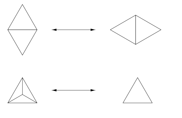
Figure 5: Ergodic set of local transformations of dynamical triangulations

The flip operation preserves the area. It is ergodic in the ensemble of triangulations with a fixed area [41, 100]. The other two operations in the figure which remove or add a point of order three, change the area and allow for extending simulations to the grand-canonical ensemble. The three moves form a set of moves called in general the $(p,q)$ moves [101]. The first argument $p$ corresponds to the number of triangles before the transformation, and $q$ after it. Note, that the four triangles, $p+q=4$, form a tetrahedron when glued together [24]. This observation was used to generalize these transformations to higher dimensions, as we shall see later. There is also another ergodic set of transformations, called the split and joint operations, also used in update schemes [102]. The two sets are equivalent.

The standard algorithm was extensively tested in two dimensions. The distribution of triangulations generated by the algorithm is in perfect agreement with the analytic formula for the diagram enumeration. Numerical measurements of the critical exponents of the statistical models $0<c\leq 1$ are in excellent agreement with the KPZ results [103]. The agreement extends beyond the critical region as is shown by the comparison of the numerical results for the Ising model on the dynamical triangulations and the analytic results of the two matrix model [77, 104]. This can be treated as a proof for the practical ergodicity of the Monte Carlo algorithms. This practical proof is in a sense stronger than the mathematical proof which only states the existence of a Markov chain between any two configurations which may of course not suffice for practical purposes.

The $(p,q)$ moves have a natural generalization to higher dimensional simplicial manifolds [101]. In four dimensional case there are five moves $p+q=6$, $p=1,\dots,5$. Geometrically they can be viewed as a substitution of $p$ 4-simplices from the triangulation by $q$ new simplices being a complementary part of the boundary of a 5-simplex. One can show that the $(p,q)$ moves are equivalent to the Alexander transformations [100] known to be ergodic in the set of combinatorially equivalent simplicial manifolds with a fixed topology. As in two dimensions, one can show the practical ergodicity of the algorithm [105]. One has to keep in mind, however, as prompted in [106], that the recognizability conjecture states that for some topologies a fraction of manifolds accessible by a Markov chain may scale to a number less than one in the large volume limit. This may systematically bias the analysis of the finite size scaling.

The ergodicity and the detailed balance condition leave a large freedom for the invention of optimal algorithms. The local update schemes are known in general to suffer from the slowing down, decreasing the algorithmic efficiency. The reason lies in the random–walk nature of local changes – namely, many changes are undone by successive steps of the algorithm. A general strategy to cure the problem is to implement algorithms focusing directly on physically important modes. This strategy has been frequently used in the standard field theoretical Monte Carlo simulations as for instance in the multi scale or cluster algorithms [107, 108].

Figure 6: Elementary step of the baby universe surgery on dynamical triangulations.

As discussed, typical random surfaces from the branched polymer phase or from the Liouville phase are populated with baby universes forming self similar trees [91]. The idea to use the tree structure in the update scheme leads to the baby universe surgery algorithm [109] . The algorithm is in fact very simple as depicted in figure 6. One finds a minimal neck on the surface, cuts the surface along the neck, removes the corresponding minbu and pastes it into a randomly chosen place on the rest of the surface. Reshuffling minbus speeds up the algorithm dynamics by decorrelating the tree branches.

A typical quantity characterizing the efficiency is the autocorrelation time. It tells us, roughly speaking, how many sweeps of the algorithm are needed to decorrelate the measurements of a given observable. The rise of the integrated autocorrelation time $\tau$ for large system sizes $A$ is controlled by the dynamical critical exponent $z$ :

$$\tau\sim A^{z}$$ (5.2)

In the table 2 we present the comparison of values of the dynamical exponent $z$ for the standard algorithm and a hybrid of the standard algorithm with the minbu surgery for various observables measured in the model with one scalar field. The values of the exponent $z$ get generally reduced if one supports the algorithm by the minbu surgery [109]. This improves significantly the algorithm dynamics. The baby universe surgery is also applied to simulate higher dimensional simplicial manifolds in the elongated phase [50, 93].

quantity	$z_{local}$	$z_{hybrid}$
$d$	1.06(3)	0.76(3)
$d_{xy}$	0.81(6)	0.14(2)
$r$	1.4(1)	0.50(3)

Table 2: The dynamical exponent for the standard local algorithm and the hybrid with the baby universe surgery, for the simulations of surfaces with $c=1$, for the averaged internal distance between points : $d$, the distance between two given points : $d_{xy}$ and the gyration radius : $r$. One sees a large reduction of the exponent $z$ when one adds the surgery to the update scheme.

Apart from the dynamical Monte Carlo techniques described above, in some particular cases there are the so-called static algorithms. They sample directly the static distribution $e^{-S}$ without using an auxiliary Markov chain. Thus, they are free of the dynamical slowing down. Example of such an algorithm is a recursive sampling technique, applicable for $c=0,-2$. In these cases there are known analytic formulas for the diagram enumeration which allow one to directly construct the diagrams weighted by the static distribution $e^{-S}$ [97, 110].

The numerical algorithms for sampling of random geometries have become a well established method allowing for studying triangulations with sizes ranging up to million triangles or hundreds of thousands of 4-simplices in the four dimensional case.

6 Simplicial gravity

Simplicial gravity is an attempt to formulate the quantum theory of gravity. It is a part of a larger programme based on the assumption that one can apply the same set of fundamental principles as in field theory, to quantize gravity. Following these lines one tries to apply the Euclidean version of the Feynman formalism as already described for the two dimensional gravity (4.1). There are many conceptual problems related to the Euclidean formulation like for example the lack of formal conditions which would ensure that we can reconstruct the Minkowskian quantum gravity. This is, however, a part of a more general difficulty, namely that we do not know how to formulate the Minkowskian quantum gravity, so we do not know what exactly should be reconstructed. The role of the topology is also not clear. And again, the problem is more general since we can not classify four dimensional topologies. Finally, there is a problem with the unboundedness of the action coming from the conformal mode. This problem, fortunately, is automatically cured by the discretization scheme. Having all these difficulties in mind let us formulate in the beginning a more modest aim, to define consistently the Feynman integral over the Riemannian structures with a fixed topology. Now the measure problem arises. It is much more pronounced in four dimensions than it is in two. One way to bypass it is to formulate the theory perturbatively in terms of the Gaussian measure which is well defined. The perturbation theory obtained in this way is however not renormalizable and the treatment fails. One can improve the convergence of the perturbative diagrams at large momenta by resummation techniques but then one encounters problems with unitarity [111].

One attempt of the nonperturbative formulation of quantum gravity is based on the $2+\epsilon$ expansion [3, 112, 113]. The situation is somewhat similar to the nonlinear sigma model [114] where the perturbative treatment does not work above two dimensions but one can find a well defined nonperturbative fixed point in terms of the $2+\epsilon$ expansion. The $2+\epsilon$ expansion may in principle be applied to gravity but in this case one has two conceptual difficulties. First of all, $\epsilon$ equal two is not a small parameter, and second of all, two dimensional integrals appearing as coefficients in the $\epsilon$-expansion are not able to reproduce the whole content of higher dimensional gravity.

Another way to define the Feynman integrals nonperturbatively is provided by the lattice regularization. In this context it was proposed in [6, 7]. This is a generalization of the dynamical triangulation approach from two [15, 16, 17] and three dimensions [23, 24, 25].

A lattice formulation allows the use of the statistical ideas and techniques to calculate quantum amplitudes which in the statistical language correspond to some averages over the statistical ensembles. The standard procedure of the the statistical approach is well established. Namely, given a model one addresses the following questions :

1. does the model posses a well defined thermodynamic limit,

2. what is the phase structure of the model,

3. can one define a lattice independent continuum limit.

The last issue is related to the existence of a continuous phase transition and the infinite correlation length of some physical excitations which would be independent of the short-range details of the lattice.

Let us follow these lines in the presentation. We consider an ensemble of simplicial manifolds with a fixed topology. Four dimensional simplicial manifold consists of equilateral 4-simplices glued together in such a way that each two neighbouring simplices share a three dimensional 3-simplex. The neighbourhood of each vertex is homomorphic to the $4$-ball.

As discussed in the previous sections, the sum over one dimensional graphs could be generated by the perturbative expansion of the scalar field theory while the sum over two dimensional graphs by the matrix field theory. The extension of this idea to the tensor model to generate four dimensional simplicial manifolds does not work, though it might seem to be an evident generalization at a first glance. The reason is that the perturbation expansion of tensor models generates graphs with fluctuating topology. Even worse, the topology of diagrams fluctuates locally so that such diagrams do not correspond to manifolds [11]. For the time being the only method to investigate the sum over the ensemble of four dimensional simplicial manifolds are the numerical simulations combined with the standard statistical data analysis.

One considers the grand-canonical ensemble of simplicial manifolds with a given topology. The partition function reads :

$${\cal Z}(\kappa_{4},\kappa_{0})=\sum_{T}\frac{1}{C[T]}e^{\kappa_{0}N_{0}[T]-\kappa_{4}N_{4}[T]}$$ (6.1)

The discretized Einstein-Hilbert action (1.6) reproduces in the naive continuum limit the continuum counterpart (1.3). For convenience we substituted the number of triangles $N_{2}$ from the formula (1.6) by the number of vertices $N_{0}$. This can be done since the numbers $N_{i}$ of $i$-simplices on the manifold are linearly related by the Euler and Dehn-Somerville relations, which leave only two independent $N_{i}$’s. In particular, for the four dimensional sphere $N_{0}$ and $N_{2}$ are related by $N_{2}=2(N_{0}+N_{4}-2)$.

One can rewrite the grand-canonical partition function as a sum :

$${\cal Z}(\kappa_{4},\kappa_{0})=\sum_{N_{4}}Z(N_{4},\kappa_{0})e^{-\kappa_{4}N_{4}}$$ (6.2)

where $Z(N_{4},\kappa_{0})$ are the partition functions for the canonical ensembles which have a fixed volume $N_{4}$. One can go one step further and express $Z(N_{4},\kappa_{0})$ in terms of the state density $z(N_{4},N_{0})$ :

$$Z(N_{4},\kappa_{0})=\sum_{N_{4}}e^{\kappa_{0}N_{0}}z(N_{4},N_{0})$$ (6.3)

The thermodynamic limit exists if the free energy density has a well defined large $N_{4}$ limit. This means that the function $\Delta$ in the formula

$$\log Z(N_{4},\kappa_{0})=N_{4}\{f(\kappa_{0})+\Delta(N_{4},\kappa_{0})\}$$ (6.4)

must be a finite size correction $\Delta$ which vanishes for large volumes $N_{4}\rightarrow\infty$ :

$$\Delta(N_{4},\kappa_{0})\rightarrow 0.$$ (6.5)

so that in the limit $N_{4}\rightarrow\infty$, the free energy density $\log Z(N_{4},\kappa_{0})/N_{4}$ is a function of $\kappa_{0}$ only.

One can show that if the function $\Delta$ vanishes for one finite value of $\kappa_{0}$ it does so for all other. The function $\Delta$ was studied for different values of the coupling $\kappa_{0}$ [55, 56, 57, 58]. In particular it was found that for $\kappa_{0}=0$ the function delta scales as $\Delta\sim N_{4}^{x}$ where $x=0.5(2)$ for manifolds with spherical and toroidal topology [58]. This is a numerical proof for the existence of the thermodynamic limit. For $\kappa_{0}=0$ the partition function $Z(N_{4},\kappa_{0}=0)$ is a sum of all manifolds without an extra weight. This sum is an object of intensive mathematical studies [115, 116]. The goal of these studies is to prove the existence of the exponential bound $Z(N_{4},\kappa_{0}=0)\leq e^{cN_{4}}$. Of course, this is equivalent to the existence of the thermodynamic limit of the model. So far there is no such proof and one has to rely on the numerical results.

One can show, as we shall see later, that the pseudo-critical value $\kappa_{0,cr}$, at which the system enters the generic branched polymer phase is finite, or more precisely, it is bounded from above by a finite value independent of $N_{4}$. On the other hand, it is known that the branched polymer phase has a well defined thermodynamic limit. Combining these two facts, one concludes that there exists a finite value of $\kappa_{0}$, for which the equation (6.5) is fulfilled. This suffices to end the proof of existence of the thermodynamic limit. In our opinion this is the strongest numerical evidence for the existence of the thermodynamic limit. What is nontrivial here is that the pseudo-critical value $\kappa_{0,cr}$ does not move to infinity when $N_{4}$ is increased as would happen if there was no thermodynamic limit.

Numerical simulations were performed for three topologies : the sphere $S^{4}$ and tori $S^{1}\times S^{1}\times S^{1}\times S^{1}$ , $S^{3}\times S^{1}$. In all these cases the free energy density $f(\kappa_{0})$ was found numerically to have the same thermodynamic limit [58].

Let us now outline the basic facts gathered using the computer simulations about the phase structure of the model.

Simplicial gravity has two phases, crumpled and elongated, named to reflect their geometrical properties. The elongated phase corresponds essentially to the branched polymer phase [50]. In this phase typical simplicial manifolds are populated with baby universes which form the generation trees. The susceptibility exponent is $\gamma=1/2$. The puncture-puncture correlation function is in this phase given by the universal formula (2.16), (2.17) for branched polymers.

Figure 7: Minbu trees for configurations taken at random from the elongated phase (left) and the crumpled phase (right). Each link on the tree corresponds to a minimal neck on the simplicial manifold, and the end points of the link correspond to two parts of the simplicial manifold on both sides of the minimal neck. The number of links emerging from a vertex of the tree corresponds to the number of minimal necks found directly on the part of simplicial manifold associated with the vertex. The trees carry only topological information about the connectivity of minbus. The vertical ordering seen on the picture results from visualization procedure and has no relevance for the tree structure. The tree on the left hand side has many generations and no distinguishable points. The tree on the right hand size is short and has one singular vertex drawn as a root of the tree. There are so many links emerging directly from the singular vertex that the visualization procedure failed to draw them as separate lines and instead drew a densely covered triangle.

The only dependence on $\kappa_{0}$ enters the formula through one universal parameter $a$ as in the formula (2.16). In the figure 7 we show the minbu trees constructed on simplicial manifolds picked up randomly from two different phases of simplicial gravity. The tree on the left hand side comes from the branched polymer phase. A vertex on the tree corresponds to a minbu and a link to the minimal neck between neighbouring minbus. One can define a distance between vertices on such a tree as a number of links between them. Then one can measure a minbu-minbu correlation function analogous to the puncture-puncture correlation function [39]. The results fit perfectly the branched polymer correlation function (2.16) as shown in figure 8. This means that the minbu trees are indeed branched polymers.

Figure 8: The minbu-minbu correlation function measured on minbu trees in the elongated phase of simplicial gravity (dashed line), compared with the universal formula $G(r)\sim 2are^{-ar^{2}/N}$ for the branched polymers (solid line) (2.16).

The branching structure of minbus collapses when the system enters the crumpled phase. The collapse is related to the appearance of a singular vertex on the minbu tree [37, 38]. On the tree on the right hand side in figure 7, the tree has only few generations and one vertex has many branches. This is the singular vertex. One can check that the number of branches emerging from the singular vertex grows with the total number of minbus. This is shown in figure 9.

Figure 9: The distribution of the minbu orders in the crumpled phase of simplicial gravity at $k0=1.0$ for three different $N_{4}=4000,8000,16000$. The position of the peak corresponding to the singular minbu vertex shifting proportionally to $N_{4}$.

To distinguish this minbu from the rest, one calls it the mother universe. The volume of the mother universe grows extensively with the total volume of the simplicial manifold [39]. The reason for this rapid growth is related to the singular vertices residing on the mother universe. There are two singular vertices at a distance one. They form a singular link [38]. The volume of the neighbourhood of the singular vertices grows proportionally to the total volume. The situation is analogous to collapsed branched polymers. Simplicial manifolds have infinite Hausdorff dimension in this phase.

Let us finish the survey of properties of the model by describing what happens at the phase transition. The standard way of investigating the behaviour of a model at a phase transition is to perform the finite size analysis of quantities related to derivatives of the free energy. For the transition driven by $\kappa_{0}$ one investigates the second cumulant :

$$c_{2}(\kappa_{0},N_{4})=\frac{1}{N_{4}}\frac{\partial^{2}F(N_{4},\kappa_{0})}{\partial\kappa_{0}^{2}}=\frac{\langle N_{0}^{2}\rangle-\langle N_{0}\rangle^{2}}{N_{4}}$$ (6.6)

which has an interpretation of the heat capacity and is a measure of thermodynamic fluctuations. The cumulant is related to the integrated correlation function of the curvature so its behaviour indirectly measures the signal from the two point function [51, 117]. In particular, if the transition is second order, this signal may be related to the occurrence of long range correlations in the system.

In the thermodynamic limit, $N_{4}\rightarrow\infty$, the fluctuations are expected to approach a $N_{4}$–independent value $c_{2}(\kappa_{0})$ except at the transition point where the large $N_{4}$ behaviour is approximately given by the finite size scaling formula :

$$c_{2}(\kappa_{0},N_{4})\sim N_{4}^{\alpha/{d_{H}\nu}}f\big{(}(\kappa_{0}-\kappa_{0,cr})N_{4}^{1/d_{H}\nu}\big{)}$$ (6.7)

where $\alpha$ and $\nu$ are the standard critical indices. They are related by the Fisher scaling relation $\alpha=2-d_{H}\nu$. The value of the product $d_{H}\nu$ is bounded by the thermodynamic inequality : $1\leq d_{H}\nu$. In the limiting case $d_{H}\nu=1$, the transition is of first order. In this case the exponent $\alpha=1$. The prefactor in the scaling formula (6.7) grows linearly with $N_{4}$. When $1<d_{H}\nu<2$ and $0<\alpha<1$, the transition is of second order. The prefactor in (6.7) grows as a power of $N_{4}$, between zero and one. Finally, when $d_{H}\nu>2$ and $\alpha<0$, the prefactor in (6.7) does not grow with $N_{4}$ and then $c_{2}$ approaches a finite constant at the transition.

Finite size analysis of the second cumulant shows that the large $N_{4}$ behaviour is in agreement with the first order scaling [51]. The observed linear rise with the volume of the maximum of the heat capacity is related to the latent heat. Hence one expects a double peak structure in the $N_{0}/N_{4}$ distribution. Indeed, such a structure has been found (see figure 10)

Figure 10: The distribution of $N_{0}$ at $\kappa_{0}=1.258$ for $N_{4}=32000$ measured in the computer simulations. The vertical axis corresponds to the number of entries for a given $N_{0}$.

at some pseudo-critical value of $\kappa_{0}$ [51, 52].

To summarize, there are two phases separated by a first order phase transition. This means that there is no continuum theory associated with this critical point. We shall discuss the issue of the continuum theory at the end of the section.

Before doing this let us come back to the thermodynamics. The scaling properties of the elongated phase are exactly the same as those of the generic branched polymers as shows the analysis of the minbu-minbu correlations. The analysis of the minbu trees suggests that the correspondence to branched polymers can be extended to the crumpled phase as well, when taken with some precaution [39]. Indeed, the distribution of vertex orders on the minbu trees has a peak departing from the rest of the distribution when the number of minbus grows. Compare the figure 2 and the figure 9.

The application of the balls-in-boxes model can be extended beyond the effective theory for minbu trees. Namely, the model gives also a plausible explanation of the appearance of the singular vertices on the simplicial manifold. If one repeats the same line of arguments as in the section on random surfaces, one obtains a constrained mean field approximation for the distribution of the vertex orders of simplicial manifolds. The partition function for the ensemble with $N_{0}$ vertices and $N_{4}$ 4-simplices is approximated as follows :

$$z(N_{4},N_{0})=\sum_{\{q_{i}\}}p(q_{1})\dots p(q_{N_{0}})\delta(q_{1}+\dots q_{N_{0}}-5N_{4})$$ (6.8)

and one ends up with the balls-in-boxes model with the density $\rho=5N_{4}/N_{0}$. If one lowers $N_{0}$, keeping $N_{4}$ fixed, the density decreases and one triggers the transition to the collapsed phase with singular vertices. The mean field approximation assumes the independence of orders of vertices as a first approximation. The approximation does not give any particular form of $p(q)$. Some numerical estimates for the weights $p(q)$ were given in [53]. In the standard numerical setup one uses the $(\kappa_{0},N_{4})$ ensemble. In this ensemble, the average $N_{0}$ grows with $\kappa_{0}$. Thus one expects the low density phase for large $\kappa_{0}$ and the high density for small $\kappa_{0}$. Indeed this is the case. Moreover the $(\kappa_{0},N_{4})$ ensemble corresponds to the $(\kappa,N)$ ensemble of the balls-in-boxes model (3.18) which has a discontinuous phase transition with a double peak distribution of $M/N$ (figure 3). As we have seen, this is what one observes in the numerical data for simplicial gravity, too (figure 10). Introducing some next order corrections to the mean-field approximation by taking into account the geometrical structure of four dimensional simplicial manifolds one can explain appearance of the singular links as well [39].

The phase structure of the model discussed in the present section resembles the phase structure of random surfaces above $D=c=1$. The respective line in the $(\alpha,D)$ plane (see figure 4) crosses only the branched polymer phase and the collapsed phase, exactly as in four dimensions. We know that in two dimensions, the system enters the branched polymer phase when the entropy of spiky conformal configurations becomes dominant. The entropy is confronted with the measure term whose dominance would mean that the system is in the collapsed phase. There is no other possibility on the line above $D=1$. To open the physical window for the gravity phase in two dimensions, one has to change the matter content of the theory by decreasing the central charge $c=D$ below one. This is an important lesson.

One can similarly expect that the phase structure of four dimensional simplicial gravity depends on the matter dressing of the theory [35, 63]. Outside the physical window the system is realized either by the branched polymer phase or by the collapsed phase. The question is now how to find the window for the gravitational phase. To start with, one can formulate a more moderate goal, and ask how to prevent the system from entering the collapsed or the branched polymer phase. This problem has been addressed recently [59, 63]. Again it is useful to refer to the analogy with the two dimensional case. The instability of the Liouville phase is caused by the entropy of spiky configurations of the conformal field [60, 61, 62]. One can now try to repeat the arguments to the effective action for the conformal mode in four dimensions [59]. The coefficient standing in front of the conformal anomaly :

$$Q^{2}=\frac{1}{180}(N_{S}+\frac{11}{2}N_{F}+62N_{V}-28)\,+Q^{2}_{grav}$$ (6.9)

depends on the matter content of the theory through the number of scalar fields $N_{S}$, vector fields $N_{V}$ and fermions $N_{F}$, coupled to gravity [118]. The $-28$ comes from the ghost sector. The contribution from gravitons $Q^{2}_{grav}$ has not been calculated since it strongly depends on the ultraviolet physics for which the perturbative treatment fails. The coefficient $Q^{2}$ plays the role of the effective central charge in the theory and it enters the estimates of the free energy of spiky conformal configurations. The reasoning is analogous as for the Liouville action in two dimensions [60, 61, 62]. It turns out, that for $Q^{2}$ less than a certain critical value : $Q^{2}<Q^{2}_{crit}$ the system is dominated by the entropy of spikes which means that the system is in the branched polymer phase. Hence, contrary to two dimensions, one expects that the fewer degrees of freedom coupled to four dimensional gravity, the higher is the probability for the system to be in the branched polymer phase. An inspection of the formula (6.9) shows that the strongest increase of the conformal charge $Q^{2}$ comes from vector fields. In the paper [59], the value of $Q^{2}_{crit}-Q^{2}_{grav}$ was estimated to be of order unity. If this is true, this means that by adding few generations of vector fields, one should be able to prevent the branching induced by the entropical instability of the conformal factor. Indeed, contrary to the previous investigations where some other matter fields were used [27, 69, 70, 71], which did not affect significantly the phase structure of simplicial gravity, the recent simulations with a varying number of vector fields [63] have shown that, when three vector fields are minimally coupled to gravity, the model has no branched polymer phase. Instead a new phase is created, where the value of the susceptibility exponent is negative, similarly as in the Liouville phase of the two dimensional gravity. Now we can readdress the question about the existence of a critical point in the extended model with the matter fields and about the order of the phase transition.

To summarize, statistical physics of four dimensional complexes with the simplest geometrical action depending on the number of points and the number of four simplices is well understood. It is, however, not related to the continuum physics and we understand why. We hope that the problem can be cured by extending the phase structure of the model by adding the appropriate matter fields.

Summary

We have reviewed statistical models of random lattices used as a regularization of the problem of summing over the internal random geometry of one, two and four dimensional objects. The degree of difficulty in solving the problem grows with the dimensionality of the system, as one might have naively expected. On the other hand, we have shown that there are some common mechanisms and features, like the geometrical collapse or the existence of the branched polymer phase, which are almost independent of the dimensionality of the problem. Indeed, although the collapsed phase looks slightly different in one, two or four dimensions, the primary feature, namely that it is related to the existence of singular vertices created as a surplus anomaly, is common for all cases. The same universality can be found in the branched polymer phase.

The most interesting part of the theory, ie the physical window, where the discrete models can be related to the continuum physics, is dimension dependent.

In two dimensions, in the Liouville phase, related to the continuum physics, the universal properties of the model, like the scaling dimensions, are entirely determined by a single parameter being the conformal charge of the theory. There is a discrete series of unitary models of conformal matter coupled minimally to gravity with the central charge in the range between zero and one which have a realization as statistical models on dynamical triangulations. The Liouville phase is basically a theory of the conformal factor.

The situation is more complicated in four dimensions where the theory is much more complex and requires extending the analysis beyond the conformal sector. But already the analysis of the conformal sector imposes some restrictions on the combinations of the numbers of various fields needed to avoid the conformal instability. One expects that there are some other conditions one has to impose on the number of generations of various fields, which lead to a specific mixture of fields for which the theory is well defined.

References

- [1] Gauge Fields and Strings by A.M. Polyakov, Harwood Academic Publishers 1987.
- [2] A.M. Polyakov, Phys. Lett. B103 (1981) 207.
- [3] S. Weinberg, in General relativity, an Einstein Centenary Survey, eds. S.W. Hawking and W. Israel, Cambridge University Press, 1979.
- [4] S. Hawking, in General relativity, an Einstein Centenary Survey, Ed. S.W. Hawking and W. Israel, Cambridge University Press, 1979.
- [5] D. Weingarten, Nucl. Phys. B210 (1982) 229.
- [6] M. Agishtein and A.A. Migdal, Mod. Phys. Lett. A7 (1992) 50 ; Nucl. Phys. B385 (1992) 395.
- [7] J. Ambjørn and J. Jurkiewicz, Phys. Lett. B278 (1992) 50.
- [8] Ph.E. Gibbs, hep-th/9510042.
- [9] F. David, Proc. Les Houches Summer School, Session LVII (1992).
- [10] J. Ambjørn, Proc. Les Houches Summer School, Session LXII (1994).
- [11] P. Ginsparg and G. Moore, Lectures given at TASI summer school, Boulder CO, hep-th/9304011.
- [12] V. Knizhnik, A. Polyakov and A. Zamolodchikov, Mod. Phys. Lett A3 (1988) 819.
- [13] F. David, Mod. Phys. Lett. A3 (1988) 1651.
- [14] J. Distler and H. Kawai, Nucl. Phys. B321 (1989) 509.
- [15] F. David, Nucl. Phys. B257 (1985) 45, Nucl. Phys. B257 (1985) 543.
- [16] V.A. Kazakov, I. Kostov and A.A. Migdal, Phys. Lett. B157 (1985) 295; Nucl. Phys. B275 (1986) 641.
- [17] J. Ambjørn, B. Durhuus and J. Fröhlich, Nucl. Phys. B257 (1985) 433; Nucl. Phys. B270 (1986) 457.
- [18] E. Brezin and V.A. Kazakov, Phys. Lett. B236 (1990) 144.
- [19] M. Douglas and S. Shenker, Nucl. Phys. B335, (1990) 635.
- [20] D. Gross and A.A. Migdal, Phys. Rev. Lett. 64 (1990) 127.
- [21] H. Kawai, N. Kawamoto, T. Mogami and Y. Watabiki, Phys. Lett. B306 (1993) 19.
- [22] J. Ambjørn and Y. Watabiki, Nucl. Phys. B445 (1995) 129.
- [23] M.E. Agishtein and A.A. Migdal, Mod. Phys. Lett. A6 (1991) 1863.
- [24] B. Boulatov and A. Krzywicki, Mod. Phys. Lett A6 (1991) 3005.
- [25] J. Ambjørn and S. Varsted, Phys. Lett. B266 (1991) 285.
- [26] J. Ambjørn, Z. Burda, J. Jurkiewicz and C.F. Kristjansen, Phys. Lett. B297 (1992) 253.
- [27] J. Ambjørn, Z. Burda, J. Jurkiewicz and C.F. Kristjansen, Phys. Rev. D48 (1993) 3695.
- [28] S. Catterall, J. Kogut and R. Renken, Phys. Lett. B328 (1994) 277.
- [29] B. V. De Bakker and J. Smit, Phys. Lett. B334 (1994) 304.
- [30] B. Brugmann and E. Marinari, Phys. Rev. Lett. 70 (1993) 1908.
- [31] J. Ambjørn, B. Durhuus, J. Fröhlich and P. Orland, Nucl. Phys. B270 (1986) 457.
- [32] J. Ambjørn, B. Durhuus and T. Jonsson, Phys. Lett. B244 (1990) 403.
- [33] P. Bialas, Phys. Lett. B373 (1996) 289.
- [34] P. Bialas and Z. Burda, Phys. Lett. B384 (1996) 75.
- [35] J. Jurkiewicz and A. Krzywicki, Phys. Lett. B392 (1997) 291.
- [36] P. Bialas, Z. Burda and D. Johnston, Nucl. Phys. B493 (1997) 505.
- [37] T. Hotta, T. Izibuchi and J. Nishimura, Prog. Theor. Phys. 94 (1995) 263; Nucl. Phys. B. (Proc. Suppl.) 47 (1996) 609.
- [38] S. Catterall, J. Kogut, R. Renken and G. Thorleifsson, Nucl. Phys. B468 (1996) 263.
- [39] P. Bialas, Z. Burda, B. Petersson and J. Tabaczek, Nucl. Phys. B495 (1997) 463.
- [40] A. Krzywicki, Nucl. Phys. B (Proc. Suppl.) 4 (1988) 64.
- [41] D.V. Boulatov, V.A. Kazakov, I.K. Kostov and A.A. Migdal, Phys. Lett. B174 (1986) 87; Nucl.Phys. B275 (1986) 641.
- [42] J. Ambjørn, B. Durhuus and J. Fröhlich, Nucl. Phys. B275 (1986) 161.
- [43] P. Bialas and Z. Burda, hep-lat/9707028, to appear in Phys. Lett. B.
- [44] P. Bialas, Z. Burda and D.A. Johnston, hep-lat/9709056, to appear in Nucl. Phys. B (Proc. Suppl.), Lattice 97.
- [45] V.A. Kazakov, Phys. Lett. A119 (1986) 140.
- [46] M. Douglas, Phys. Lett. B238 (1990) 238.
- [47] J. Ambjørn, K. Anagnostopoulos, T. Ichihara, L. Jensen, N. Kawamoto, Y. Watabiki and K. Yotsuji, hep-lat/9706009.
- [48] J. Ambjørn, K. Anagnostopoulos and G. Thorleifsson, hep-lat/9709025, to appear in Nucl. Phys. B (Proc. Suppl.), Lattice 97.
- [49] M. Bowick, hep-lat/9710005, to appear in Nucl. Phys. B (Proc. Suppl.), Lattice 97.
- [50] J. Ambjørn and J. Jurkiewicz, Nucl. Phys. B451 (1995) 643.
- [51] P. Bialas, Z. Burda, A. Krzywicki and B. Petersson, Nucl. Phys. B472 (1996) 293.
- [52] B.V. de Bakker, Phys. Lett. B389 (1996) 238.
- [53] S. Catterall, J. Kogut and R. Renken, hep-lat/9709007.
- [54] S. Bilke, Z. Burda and J. Jurkiewicz, Comp. Phys. Comm. 85 (1995) 278.
- [55] B. V. de Bakker, PhD Thesis, Amsterdam, hep-lat/9508006.
- [56] J. Ambjørn and J. Jurkiewicz, Phys. Lett. B335 (1994) 355.
- [57] B. Brugmann and E. Marinari, Phys. Lett. B349 (1995) 35.
- [58] S. Bilke, Z. Burda and B. Petersson, Phys. Lett. B395 (1997) 4.
- [59] I. Antoniadis, P.O. Mazur and E. Mottola, Phys. Lett. B394 (1997) 49.
- [60] M.E. Cates, Europhys. Lett. 8 (1988) 719.
- [61] A. Krzywicki, Phys. Rev. D41 (1990) 3086.
- [62] F. David, Nucl. Phys. B368 (1992) 671.
- [63] S. Bilke, Z. Burda, A. Krzywicki, B. Petersson, J. Tabaczek and G. Thorleifsson, hep-lat/9710077.
- [64] T. Regge, Nuovo Cimento 19 (1961) 558.
- [65] P. Menotti, hep-lat/9709101, to appear in Nucl. Phys. B (Proc. Suppl.), Lattice 97.
- [66] C. Holm and W. Janke, Phys. Lett. B375 (1996) 69.
- [67] J. Ambjørn, J. Jurkiewicz and C.F. Kristjansen, Nucl. Phys. B393 (1993) 601.
- [68] J. Ambjørn, Z. Burda, J. Jurkiewicz and C.F. Kristjansen, Acta Phys. Polon. B23 (1992) 991.
- [69] J. Ambjørn, S. Bilke, Z. Burda, J. Jurkiewicz and B. Petersson, Mod. Phys. Lett. A9 (1994) 2527.
- [70] S.M. Catterall, J.B. Kogut and R.L. Renken, Nucl. Phys. B389 (1993) 601.
- [71] S.M. Catterall, J.B. Kogut and R.L. Renken, Nucl. Phys. B422 (1994) 677.
- [72] J. Ambjørn, J. Jurkiewicz and Y. Watabiki, J. Math. Phys. 36 (1995) 6299.
- [73] G. Roepstorff and L. Schulman, J. Stat. Phys 34 (1984) 35.
- [74] B. Gaveau and L Schulman, J. Phys. A20 (1987) 2865.
- [75] H. Kawai, N. Tsuda and T. Yukawa , Nucl. Phys. (Proc. Suppl.) 47 (1996) 653 ; Nucl. Phys. (Proc. Suppl.) 53 (1997) 777.
- [76] D.V. Boulatov and V.A. Kazakov Phys. Lett. B186 (1987) 379.
- [77] Z. Burda and J. Jurkiewicz, Acta Phys. Polon. B20 (1989) 949.
- [78] G. ’t Hooft, Nucl. Phys. B72 (1974) 461.
- [79] B. Durhuus, Nucl. Phys. B426 (1994) 203.
- [80] J. Ambjørn, G. Thorleifsson and M. Wexler, Nucl. Phys. B439 (1995) 187.
- [81] J. Ambjørn, Z. Burda, J. Jurkiewicz and B. Petersson, Phys. Lett. B341 (1995) 286.
- [82] M. Wexler, Nucl. Phys. B438 (1995) 629.
- [83] M. Wexler, Mod. Phys. Lett. A8 (1993) 2703.
- [84] P.B. Wiegmann, Nucl. Phys. B323 (1989) 330.
- [85] G.P. Korchemsky, Phys. Lett. B296 (1992) 323.
- [86] F. David, Nucl. Phys. B487 (1997) 633.
- [87] B. Petersson and G. Thorleifsson, hep-lat/9709072.
- [88] F. David, J. Jurkiewicz, A. Krzywicki and B. Petersson, Nucl. Phys. B290 (1987) 218.
- [89] J. Ambjørn, B. Durhuus, T. Jonnson and G. Thorleifsson, Nucl. Phys. B398 (1993) 568.
- [90] J.P. Kownacki and A. Krzywicki, Phys. Rev. D50 (1994) 5329.
- [91] S. Jain and S. Mathur, Phys. Lett. B286 (1992) 239.
- [92] D.Johnston, J-P. Kownacki and A. Krzywicki, Nucl. Phys. B (Proc. Suppl.) 42 (1995) 728.
- [93] Z. Burda, J-P. Kownacki and A. Krzywicki, Phys. Lett. B356 (1995) 466.
- [94] N. Kawamoto, Proceedings of the 7th Nishinomiya-Yukawa Memorial Symposium: Quantum Gravity, (1993) 112.
- [95] Y. Watabiki, Nucl. Phys. B441 (1995) 119.
- [96] N. Ishibashi and H. Kawai. Phys. Lett. B314 (1993) 190; Phys. Lett. B322 (1994) 67.
- [97] N. Kawamoto, V.A. Kazakov, Y. Saeki and Y. Watabiki, Phys. Rev. Lett. 68 (1992) 2113.
- [98] J. Ambjørn, P. Bialas, Z. Burda, J. Jurkiewicz and B. Petersson, Phys. Lett. B342 (1995) 58.
- [99] J. Ambjørn, K.N. Anagnostopoulos, T. Ichihara, L. Jensen, N. Kawamoto, Y. Watabiki and K. Yotsuji, Phys. Lett. B397 (1997) 177
- [100] J.W. Alexander, Ann. Math, 31 (1930) 292.
- [101] M. Gross and S. Varsted, Nucl. Phys. B378 (1992) 367.
- [102] J. Jurkiewicz, A. Krzywicki and B. Petersson, Phys. Lett. 177B (1986) 89.
- [103] C.F. Baillie and D.A. Johnston, Mod. Phys. Lett. A7 (1992) 1519.
- [104] Z. Burda, J. Jurkiewicz and L. Kärkkäinen, Comp. Phys. Comm. 70 (1992) 510.
- [105] S. Bilke, Z. Burda, A. Krzywicki and B. Petersson, Nucl. Phys. (Proc. Suppl.) 53 (1997) 743.
- [106] R. Ben-Av and A. Nabutovsky, Commun. Math. Phys. 157 (1993) 93.
- [107] R.H. Swendsen and J.S. Wang, Phys. Rev. Lett. 58 (1987) 86.
- [108] U. Wolff, Phys. Rev. Lett. 62 (1989) 361.
- [109] J. Ambjørn, P. Bialas, Z. Burda, J. Jurkiewicz and B. Petersson, Phys. Lett. B325 (1994) 337.
- [110] M. E. Agishtein and A. A. Migdal, Int. J. Mod. Phys. C1 (1990) 165.
- [111] K. Stelle, Phys. Rev. D16 (1977) 953.
- [112] H. Kawai and M. Ninomiya, Nucl. Phys. B336 (1990) 115.
- [113] T. Aida and Y. Kitazawa, Nucl. Phys. B491 (1997) 427.
- [114] E. Brezin, J. Zinn-Justin and J.C. Le Guillou, Phys. Rev. D14 (1976) 2615.
- [115] B. Durhuus and T. Jonsson, Nucl. Phys. B445 (1995) 182.
- [116] M. Carfora and A. Marzuoli, J. Math. Phys. 36 (1995) 6253.
- [117] B. V. de Bakker and Jan Smit, Nucl. Phys. B454 (1995) 343.
- [118] S.M. Christensen and M.J. Duff, Nucl. Phys. B170 [FSI] (1980) 480.