Low temperature expansion of the gonihedric Ising model

Abstract

We investigate a model of closed $(d-1)$-dimensional soft-self-avoiding random surfaces on a $d$-dimensional cubic lattice. The energy of a surface configuration is given by $E=J(n_{2}+4k\,n_{4})$, where $n_{2}$ is the number of edges, where two plaquettes meet at a right angle and $n_{4}$ is the number of edges, where 4 plaquettes meet. This model can be represented as a $\mathbb{Z}_{2}$-spin system with ferromagnetic nearest-neighbour-, antiferromagnetic next-nearest-neighbour- and plaquette-interaction. It corresponds to a special case of a general class of spin systems introduced by Wegner and Savvidy. Since there is no term proportional to the surface area, the bare surface tension of the model vanishes, in contrast to the ordinary Ising model. By a suitable adaption of Peierls argument, we prove the existence of infinitely many ordered low temperature phases for the case $k=0$. A low temperature expansion of the free energy in 3 dimensions up to order $x^{38}$ ($x=\mbox{e}^{-\beta J}$) shows, that for $k>0$ only the ferromagnetic low temperature phases remain stable. An analysis of low temperature expansions up to order $x^{44}$ for the magnetization, susceptibility and specific heat in 3 dimensions yields critical exponents, which are in agreement with previous results.

and

1 Introduction

The so called gonihedric string was introduced by Savvidy et. al. [1, 2, 3, 4, 5] as a model for closed triangulated random surfaces. The action is given as

$$S = \sum_{\mbox{\tiny simple edges}}|\pol{X}_{i}-\pol{X}_{j}|\,\theta(\alpha_{ij})$$

$$+\>k\sum_{\mbox{\tiny common edges}}|\pol{X}_{i}-\pol{X}_{j}|\,\left(\theta(\alpha_{ij}^{(1)})+\ldots+\theta(\alpha_{ij}^{(r(2r-1))})\right).$$

The first term in (1) sums over all edges, where two triangles meet. The function $\theta(\alpha_{ij})$, which weights the edge lengths $|\pol{X}_{i}-\pol{X}_{j}|$, depends only on the angle $\alpha_{ij}$ between the neighbouring triangles such that

• $\theta(2\pi-\alpha)=\theta(\alpha)$

• $\theta(\pi)=0$

• $\theta(\alpha)\geq 0.$

If more than two triangles meet at a given edge, contributions from all pairs of triangles arise in the second term of (1). Therefore if $k>0$, this term penalizes self-intersections of the surface. Since $\theta(\pi)=0$, the gonihedric action is subdivision invariant, i.e. geometrically nearby surface configurations have similar weights. The action measures essentially the linear size of the surfaces. Configurations with long spikes are therefore suppressed. These kind of configurations destroy the convergence of the partition function for triangulated random surfaces with area action [6]. However, for $k=0$ and $\theta(\alpha)=\frac{1}{2}|\pi-\alpha|$, the gonihedric action was shown to suffer from a similar disease [7]. In this case flat “pancake like” configurations dominate such that the grandcanonical partition function fails to converge. Nevertheless numerical simulations of the canonical ensemble [8, 9, 10] show flat surfaces.

Another way to define discretized random surface theories is to consider plaquette surfaces on a cubic lattice. In this approach, not just the surface, but also the embedding space is discretized. The gonihedric string can be formulated as a model for plaquette surfaces on a euclidean lattice as was shown by Wegner and Savvidy [11, 12, 13, 14, 15, 16]. If self-overlapping of the surface is excluded (i.e. each plaquette occurs either once or not at all in the surface), the model for closed $(d-1)$-dimensional plaquette surfaces can be written as a $\mathbb{Z}_{2}$ Ising model. The spins $\sigma=\pm 1$ sit on a $d$-dimensional hypercubic lattice and the surface consists of all plaquettes of the dual lattice, which separates spins of opposite sign. The energy of a surface configuration on the lattice is now given as

$$E=\sum_{\mbox{\tiny edges}}E_{\mbox{\tiny edge}}=J(n_{2}+4k\,n_{4}),$$ (2)

where $n_{2}$ is the number of $(d-2)$-dimensional edges, where two plaquettes meet perpendicular and $n_{4}$ is the number of edges, where four plaquettes meet (see figure 1).

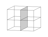
$E_{\mbox{\tiny edge}}=J$	$E_{\mbox{\tiny edge}}=0$	$E_{\mbox{\tiny edge}}=4kJ$

Figure 1: The total energy can be written as a sum over edge contributions. “Simple edges”, where two plaquettes meet perpendicular cost energy $J$. “Flat edges”, where two plaquettes of the same orientation meet, do not cost energy. If four plaquettes meet at a given edge (“double edge”), the corresponding energy contribution is $4kJ$, since according to the gonihedric string action four right angles are counted.

Expressed in terms of spin variables, the Hamiltonian reads

$$H=-Jk(d-1)\sum_{<ij>}\sigma_{i}\sigma_{j}+J\,\frac{k}{2}\sum_{<<ij>>}\sigma_{i}\sigma_{j}-J\,\frac{1-k}{2}\sum_{[ijkl]}\sigma_{i}\sigma_{j}\sigma_{k}\sigma_{l}.$$ (3)

It contains ferromagnetic nearest neighbour ($<ij>$), antiferromagnetic next nearest neighbour ($<<ij>>$) and plaquette terms ($[ijkl]$), where the corresponding couplings are tuned in a special way. Similar surface models, where the energy contains an additional term proportional to the surface area, have been considered earlier [19, 20, 21, 22, 23], in particular in connection with amphiphilic systems. However, the special choice of couplings as given in (3), has not been studied explicitly in this context. It corresponds to the disorder line as calculated in mean field approximation [22]. In two dimensions, the model can be mapped to the eight-vertex model [24]. The corresponding weights are however different from the exact solvable case. Numerical simulations indicate, that the system defined in (3) does not undergo a phase transition for $d=2$ but is in a disordered phase for all $T>0$ [25, 17]. In three dimensions the gonihedric Ising model (3) has been studied by means of mean field [26], Monte Carlo [17, 26, 27, 28] and cluster variation-Padé methods [29, 30]. At $k=0$ the model seems to undergo a first order phase transition [27], whereas for large $k$ the transition becomes second order [26, 28, 29]. Since flat edges, i.e. edges where two plaquettes of the same orientation meet, do not cost energy, the ground state is highly degenerate. For $k>0$ it consists of all configurations, where only flat domain walls are present, as long as they do not intersect. The ground state degeneracy of a finite system of size $L^{d}$ therefore increases like $d\,2^{L}$. If $k=0$, the number of ground states is even higher, since ground state planes are now allowed to intersect without an additional energy cost. Thus the degeneracy increases like $2^{dL}$ in this case. Moreover, the flipping of a whole $(d-1)$-dimensional spin layer does not change the energy of any spin configuration if $k=0$ as can easily be seen from (3), i.e.  apart from the global spin-flip symmetry the system possesses an additional layer-flip symmetry.

The outline of the paper is as follows: In section 2 we show by a suitable extension of Peierls contour method, that the layer-flip symmetry for $k=0$ is spontaneously broken at low temperature. For each ground state we find an ordered low temperature phase. In section 3 we perform a low temperature expansion around all possible ground states of the gonihedric model. The result indicates, that for $k>0$ only the ferromagnetically ordered low temperature phases remain stable, i.e. layered phases are thermodynamically suppressed at low but non zero temperature. We use Padé approximations to calculate critical exponents of the magnetization, susceptibility and specific heat from the corresponding low temperature expansions in section 4. Finally we discuss the surface tension. There is some evidence, that a roughening transition occurs below the bulk critical temperature $T_{c}$.

2 Ordered low temperature phases for $k=0$

If $k$ vanishes, then only edges, where two plaquettes meet at a right angle cost energy. These edges are surrounded by an odd number of negative spins. The flipping of a whole $(d-1)$-dimensional spin layer therefore does not change the energy, i.e. apart from the global $\mathbb{Z}_{2}$ symmetry, the Hamiltonian (3) shows an additional layer-flip symmetry at $k=0$. The ground states are the ferromagnetically ordered states and all configuration, which are connected with them by layer-flip operations. In the following we will show, that for each of these ground states there exists an ordered low temperature phase. These phases can be characterized by a non vanishing “spontaneous magnetization”, which for a finite system with $N$ spins is defined by

$$\hat{M}_{N}=\frac{\big{<}\hat{N}_{+}\big{>}-\big{<}\hat{N}_{-}\big{>}}{N}.$$ (4)

Here “$\>\hat{}\>$” refers to a boundary condition, which singles out one ground state. $\hat{N}_{-}$ denotes the number of spins, which are flipped compared to this ground state and accordingly $\hat{N}_{+}$ the number of spins, which are unchanged. To show, that $\hat{M}_{N}$ does not vanish at sufficiently low temperatures, we will use a modified Peierls argument [31, 32]. The idea is the following: Consider a finite system, where the spins at the boundary are fixed, such that one ground state is favoured (see figure 2).

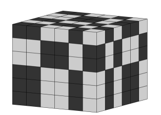
Figure 2: Starting from a ferromagnetic ground state, further ground states of the gonihedric model for $k=0$ can be constructed by swapping $(d-1)$-dimensional spin layers. The figure above visualizes such a ground state. In order to carry out the Peierls-argument, the boundary spins are fixed correspondingly.

If we now swap a little “droplet” of spins inside the volume, the amount of energy we need will be essentially proportional to the number $l$ of simple edges, which were established by swapping the spins. The simple edges form connected edge diagrams. Each overturned spin is surrounded with at least one such diagram. We can therefore estimate

$$\big{<}\hat{N}_{-}\big{>}\leq\sum_{l}\left(\frac{l}{2d(d-1)}\right)^{\frac{d}{d-2}}p(l),\qquad d\geq 3,$$ (5)

where $\left(\frac{l}{2d(d-1)}\right)^{d/(d-2)}$ is the maximum number of spins an edge diagram with $l$ simple edges encloses and $p(l)$ denotes the probability of occurrence of such a diagram. $p(l)$ can be further estimated by

$$p(l)\leq g(l)\,\mbox{e}^{-\beta Jl},$$ (6)

where $g(l)$ is the entropy factor, i.e. the number of connected edge diagrams with $l$ edges. We will show, that $g(l)$ does not grow faster than exponentially. Thus (5) will be arbitrarily small for sufficiently large $\beta$. The same type of argument was used in [33] to show the existence of a phase transition in the gonihedric model for $k>0$. The argument given there however contains a flaw, since the edge diagrams are not independent from each other, if $k>0$. We will now proceed with the details for the case $k=0$.

Consider a finite system with $N$ spins in its interior and fix the spins at the boundary, so that they belong to a ground state, as indicated in figure 2. For a configuration $\sigma$ of the spins inside the volume let $C[\mbox{\boldmath$\sigma$\unboldmath}]$ be the set of all ($(d-2)$-dimensional) edges of the dual lattice, where two ($(d-1)$-dimensional) plaquettes of the domain wall meet at a right angle. Each of these edges is surrounded by four spin, whose product is -1. Two edges in $C[\mbox{\boldmath$\sigma$\unboldmath}]$ are connected, if they have at least one ($(d-3)$-dimensional) vertex in common. $C[\mbox{\boldmath$\sigma$\unboldmath}]$ can be uniquely decomposed into connected parts:

$$C[\mbox{\boldmath$\sigma$\unboldmath}]=C_{1}^{l_{1}}\cup\ldots\cup C_{n}^{l_{n}},$$ (7)

where $C_{i}^{l}$ denotes a connected component with $l_{i}$ edges. The total energy $E[\mbox{\boldmath$\sigma$\unboldmath}]$ can be written as

$$E[\mbox{\boldmath$\sigma$\unboldmath}]=\sum_{i=1}^{n}J\,l_{i}.$$ (8)

Let $g(l)$ be the number of connected edge diagrams with $l$ edges. For each diagram we introduce a variable $\chi_{i}^{l},i=1,\ldots,g(l)$, such that

$$\chi_{i}^{l}[\mbox{\boldmath$\sigma$\unboldmath}]=\left\{\begin{array}[]{rcl}1&&\parbox[t]{128.0374pt}{if the corresponding edge diagram occurs in $\mbox{\boldmath$\sigma$\unboldmath}$}\\[14.22636pt] 0&&\mbox{otherwise}.\end{array}\right.$$ (9)

Since each spin, which is flipped compared to the ground state, is surrounded with at least one connected edge diagram, we can estimate

$$\hat{N}_{-}[\mbox{\boldmath$\sigma$\unboldmath}]\leq\sum_{l}\;\left(\frac{l}{2d(d-1)}\right)^{\frac{d}{d-2}}\>\sum_{i=1}^{g(l)}\chi_{i}^{l}[\mbox{\boldmath$\sigma$\unboldmath}].$$ (10)

Thus for the expectation value of the number of the overturned spins we obtain:

$$\big{<}\hat{N}_{-}\big{>}_{N}\>\leq\sum_{l}\;\left(\frac{l}{2d(d-1)}\right)^{\frac{d}{d-2}}\>\sum_{i=1}^{g(l)}\big{<}\chi_{i}^{l}\big{>}_{N}.$$ (11)

If we number the spin configurations, which contain $C_{i}^{l}$ by $\mbox{\boldmath$\sigma$\unboldmath}_{1},\ldots,\mbox{\boldmath$\sigma$\unboldmath}_{k}$, the expectation value $\big{<}\chi_{i}^{l}\big{>}_{N}$ can be written as:

$$\big{<}\chi_{i}^{l}\big{>}_{N} = \frac{1}{Z_{N}}\sum_{j=1}^{k}\mbox{e}^{-\beta E[\mbox{\boldmath$\scriptstyle\sigma_{j}$\unboldmath}]},$$ (12)

where

$$Z_{N} = \sum_{\mbox{\boldmath$\scriptstyle\sigma$\unboldmath}}\mbox{e}^{-\beta E[\mbox{\boldmath$\scriptstyle\sigma$\unboldmath}]}.$$ (13)

For each $\mbox{\boldmath$\sigma$\unboldmath}_{j}$ there exists a unique configuration $\mbox{\boldmath$\sigma$\unboldmath}_{j}^{*}$, which does not contain $C_{i}^{l}$ but leaves all other edge diagram unchanged, i.e.

$$E[\mbox{\boldmath$\sigma$\unboldmath}_{j}^{*}]=E[\mbox{\boldmath$\sigma$\unboldmath}_{j}]-J\,l.$$ (14)

The configurations $\mbox{\boldmath$\sigma$\unboldmath}_{1}^{*},\ldots,\mbox{\boldmath$\sigma$\unboldmath}_{k}^{*}$ are pairwise different. By restricting the partition function to these configurations, we can estimate:

$$Z_{N}\geq\sum_{j=1}^{k}\mbox{e}^{-\beta E[\mbox{\boldmath$\scriptstyle\sigma_{j}^{*}$\unboldmath}]}=\mbox{e}^{\beta Jl}\,\sum_{j=1}^{k}\mbox{e}^{-\beta E[\mbox{\boldmath$\scriptstyle\sigma_{j}$\unboldmath}]}.$$ (15)

Together with (12) this yields

$$\big{<}\chi_{i}^{l}\big{>}_{N}\>\>\leq\mbox{e}^{-\beta Jl}.$$ (16)

Hence the expectation value of the number of overturned spins is bounded by

$$\big{<}\hat{N}_{-}\big{>}_{N}\>\leq\sum_{l}\left(\frac{l}{2d(d-1)}\right)^{\frac{d}{d-2}}g(l)\;\mbox{e}^{-\beta Jl}.$$ (17)

To proceed with the argument, we need an upper bound for $g(l)$, the number of connected edge diagrams with $l$ edges. The edges in those diagrams are connected via ($(d-3)$-dimensional) vertices. What kind of edge configurations can occur at a vertex is determined by the possible configurations of the eight surrounding spins. As shown in figure 3, only four types of vertices can arise.

2-Vertex	3-Vertex	4-Vertex	5-Vertex

Figure 3: The possible edge configurations around a vertex are determined by the eight surrounding spins. Only four types of configurations can arise (modulo rotations) as shown above.

With the following method all possible connected edge diagrams can be constructed:

• Number all Vertices ($(d-3)$-dimensional plaquettes) of the lattice.

• Choose one of the $N$ lattice points, e.g. $r=(r_{1},\ldots,r_{d}),r_{i}\in\mathbb{Z}$ and attach the edge $k=\{(r_{1},r_{2},\lambda_{3},\ldots,\lambda_{d})\>|\>r_{i}\leq\lambda_{i}\leq r_{i}+1\}$. This is possible, since edges of all orientations occur in every possible diagram.

• Imagine that a connected subdiagram exists already. Consider all vertices in that diagram, where the configuration of the surrounding edges is not allowed (see figure 4). Choose the one with the lowest number and attach further edges, such that an allowed configuration results.

• Repeat constructions step 3, until all $l$ edges are attached.

The maximum number of outcomes of the procedure given above is an upper bound for $g(l)$. For construction step 2 there are $N$ possibilities. Each time we perform constructions step 3, at least one edge is added. The number of choices to complete the vertex depends on the edge configuration already present. In figure 4, we list all possibilities which can arise together with the number of choices $n(k)$ to attach $k$ edges.

$k$	$n(k)$	$k$	$n(k)$	$k$	$n(k)$	$k$	$n(k)$	$k$	$n(k)$
1	1	1	2	1	1	1	0	1	1
2	4	2	1	2	0	2	1	2	0
3	2	3	0	3	1	3	0	3	0
4	0	4	1	4	0	4	0	4	0
5	1	5	0	5	0	5	0	5	0

Figure 4: The figure shows all possibilities of incomplete vertices (modulo rotations). $n(k)$ is the number of choices to complete the vertex by adding $k$ edges.

Let $n_{\mbox{\tiny max}}(k)$ be the maximum number of choices to attach $k$ edges. The function

$$f_{r}(x):=N\,x\left(\;\sum_{k=1}^{5}n_{\mbox{\tiny max}}(k)\,x^{k}\right)^{r},$$ (18)

can now be interpreted as a generating function, which counts all connected edge diagrams with $l$ edges at least once, which can be constructed by repeating constructions step 3 r-times, i.e. the coefficient of $x^{l}$ in the series expansion of $f_{r}(x)$ is an upper bound for the number of those diagrams. Therefore an upper bound for $g(l)$ is provided by

$$g(l)\leq\frac{1}{l!}\left(\frac{d}{dx}\right)^{l}\left.\left(\;\sum_{r=0}^{\infty}f_{r}(x)\right)\>\right|_{x=0}.$$ (19)

The values $n_{\mbox{\tiny max}}(k)$ can be read off from figure 4. We find:

$$g(l) \leq \frac{1}{l!}\left(\frac{d}{dx}\right)^{l}\left.\left(\frac{N\,x}{1-(2x+4x^{2}+2x^{3}+x^{4}+x^{5})}\right)\>\right|_{x=0}$$ (20)

$$=: \frac{1}{l!}\left(\frac{d}{dx}\right)^{l}\left.G(x)\>\right|_{x=0}.$$ (21)

$G(x)$ can be written as:

$$G(x)=\frac{N\,x}{1-(2x+4x^{2}+2x^{3}+x^{4}+x^{5})}=N\,\sum_{k=1}^{5}\frac{r_{k}}{x-x_{k}}.$$ (22)

Putting this expression in (20), we obtain

$$g(l)\leq N\,\sum_{k=1}^{5}\left(-\frac{r_{k}}{x_{k}}\right)\left(\frac{1}{x_{k}}\right)^{l}.$$ (23)

The increase of $g(l)$ is dominated by the smallest $|x_{k}|=:x_{\mbox{\tiny min}}$. Hence we can further estimate:

$$g(l)\leq N\,\left(\sum_{k=1}^{5}\left|\frac{r_{k}}{x_{k}}\right|\right)\left(\frac{1}{|x_{m}|}\right)^{l}\leq N\,0.67\,(3.39)^{l}.$$ (24)

Substituting this result in (17), we find an upper bound for the density of overturned spins:

$$\frac{\big{<}\hat{N}_{-}\big{>}_{N}}{N}\>\leq\sum_{l}\left(\frac{l}{2d(d-1)}\right)^{\frac{d}{d-2}}0.67\,(3.39)^{l}\;\mbox{e}^{-\beta Jl}.$$ (25)

This inequality remains valid in the thermodynamical limit. The sum on the right hand side approaches zero, if $\beta$ tends to infinity. Therefore, for $\beta>\beta_{c}$ it will be smaller than $\frac{1}{2}$, which implies a non-zero spontaneous magnetization. This completes the proof. Note that the estimate above is only valid for $d\geq 3$. Indeed in two dimensions, the model for $k=0$ is equivalent to the 1-dimensional ordinary Ising model [12]. Thus no transition occurs in this case.

The upper bound for $\big{<}\hat{N}_{-}\big{>}_{N}$ given above can be used to calculate an upper bound for $\beta_{c}$. We find

$$\beta_{c}J\leq 1.43 \mbox{for}\quad d=3,$$

$$\beta_{c}J\leq 1.33 \mbox{for}\quad d=4.$$

The upper bound for $\beta_{c}J$ in 3 dimensions is consistent with values obtained from simulations [26, 27] ($\beta_{c}J\approx 0.505$), cluster variation-Padé approximations [29] ($\beta_{c}J\approx 0.550$) and mean field calculations [26] ($\beta_{c}J\approx 0.325$).

If $k>0$ a similar proof can not carried through, since in this case the connected edge diagrams are not independent from each other, i.e. given a configuration $\sigma$ which contains a certain edge diagram $C_{i}^{l}$, the corresponding configuration $\mbox{\boldmath$\sigma$\unboldmath}^{*}$ does not necessarily fulfil the condition

$$E[\mbox{\boldmath$\sigma$\unboldmath}^{*}]=E[\mbox{\boldmath$\sigma$\unboldmath}]-E[C_{i}^{l}],$$ (26)

where $E[C_{i}^{l}]$ denotes the energy contribution of the connected edge diagram. In going over from $\sigma$ to $\mbox{\boldmath$\sigma$\unboldmath}^{*}$, the energy can even increase by an amount $\sim l^{2}$.

3 Low temperature expansion of the free energy

If $k>0$ then the Hamiltonian (3) is no longer invariant under layer-flip operations. Only the global $\mathbb{Z}_{2}$ spin-flip symmetry remains. However flat domain walls still do not cost energy. Thus apart from the ferromagnetically ordered ground states, there are layered ground states containing flat domain walls which do not intersect. As was already mentioned in [29], the ground state contributions $Z^{(g)}$ of the total partition function

$$Z=\sum_{g}Z^{(g)}$$ (27)

are not degenerate in contrast to the $k=0$ case. Here $Z^{(g)}$ contains the ground state $g$ and all configurations, which differ from $g$ by a “small” number of spins. The lowest excitation is realized by a configuration, where one spin is flipped compared to the ground state. Since this configuration contains 12 simple edges (elementary cube), its energy is $12J$, independent of the underlying ground state. The next higher excitation is obtained by swapping an additional nearest neighbour spin. The energy of this configuration however depends on the ground state: If there is no flat domain wall present between those two spins, the energy is 16J. Otherwise four additional double edges contribute, i.e. the energy amounts to $16J+16Jk$. Thus to lowest order, layered low temperature phases seem to be energetically disfavoured [29]. In this section we will quantify this effect. For this we perform a low temperature expansion of the free energy for the three dimensional case to estimate the magnitude of each ground state contribution $Z^{(g)}$. This analysis indicates, that at low but non-zero temperature the occurrence of layered low temperature phases is indeed thermodynamically suppressed.

Consider a finite system of volume $V=L^{3}$. By ${\bf N}$ we denote the set of the $N=L^{3}$ spins inside $V$. Each excitation of a given ground state g is defined by the subset ${\bf I}\subseteq{\bf N}$ of spins, which are swapped compared to g. The excitation energy $E^{(g)}({\bf I})$ depends on g. We define the ground state contributions $Z^{(g)}_{N}$ by:

$$Z^{(g)}_{N} := \sum_{{\bf I}\subseteq{\bf N}}z^{(g)}({\bf I}),$$ (28)

where

$$\quad z^{(g)}({\bf I}) := \mbox{e}^{-\beta E^{(g)}({\bf I})}.$$ (29)

Ground states g which can be mapped onto each other by a rotation or a global spin flip yield the same $Z^{(g)}_{N}$. We therefore write:

$$Z_{N}=2\Big{(}Z_{N}^{(0)}+3\sum_{g=1}^{2^{L-1}-1}Z_{N}^{(g)}\Big{)},$$ (30)

where $g$ refers to ground states modulo rotations and global spin-flip and $g=0$ denotes the ferromagnetically ordered ground state. The logarithm of $Z^{(g)}_{N}$ can be written as:

$$\mbox{ln}(Z^{(g)}_{N})=\sum_{{\bf I}\subseteq{\bf N}}c^{(g)}({\bf I}),$$ (31)

where the cluster contributions $c^{(g)}({\bf I})$ are defined by

$$c^{(g)}({\bf I})=\sum_{{\bf J}\subseteq{\bf I}}(-1)^{(|{\bf I}|-|{\bf J}|)}\>\mbox{ln}\Big{(}\sum_{{\bf K}\subseteq{\bf J}}z^{(g)}({\bf K})\Big{)}.$$ (32)

As can easily be shown, these cluster contributions vanish, if the cluster ${\bf I}$ is not “connected”. Here we call two spins connected, if their elementary cubes have at least one edge in common. In general two spin clusters ${\bf I}_{1},{\bf I}_{2}$, which can be mapped onto each other by a translation will contribute differently, unless the translation is parallel to the ground state planes. To take care of this restricted translation invariance we introduce structural coefficients, which characterize the ground states such that the right hand side of (31) can be expanded systematically: For each ground state $g$ there exists a unique $(L-1)$-tupel $p(g)=(p_{1},\ldots,p_{L-1})$, $p_{i}=0,1$, which characterizes the sequence of ground state planes say in positive direction. $p_{i}=1$ means, that a ground state plane is present (see figure 5).

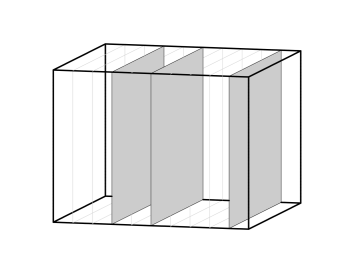
$L=10$,   $p(g)=(0,0,1,0,1,0,0,0,1)$

Figure 5: The picture above displays ground state layers within a finite volume of linear length $L=10$. The sequence of this layers in positive direction (from left to right) is described by a $(L-1)$-tupel $p$.

For $q=(q_{1},\ldots,q_{n})$, $q_{i}=0,1$, $n<=L-1$ and

$$T:=\{k\in\mathbb{N}\;|\;q_{1}=p_{k},\ldots,q_{n}=p_{k+n-1}\}.$$ (33)

we define:

$$a_{q}:=\mbox{Number of elements in $T$}.$$ (34)

Thus $a_{q}(g)$ is the number of translations, such that the sequence $q$ matches with a subsequence of $p(g)$. If $q$ does not have any elements, we set $a(g)=L$. The structural coefficients are not independent from each other, e.g. the following equations hold:

$$\begin{array}[]{rcl}a(g)&=&L\\ a_{0}(g)+a_{1}(g)&=&L-1\\ a_{00}(g)+a_{01}(g)+a_{10}(g)+a_{11}(g)&=&L-2\\ &\vdots&\end{array}$$ (35)

Using the structural coefficients, we can now write:

$$\lim_{L\to\infty}\frac{\mbox{ln}(Z_{N}^{(g)})}{N}=\lim_{L\to\infty}\frac{1}{L}\Big{(}a(g)f+a_{0}(g)f_{0}+a_{1}(g)f_{1}+a_{00}(g)f_{00}+\ldots\Big{)}.$$ (36)

In this expression $f$ denotes the sum of all cluster contributions of widths 1, i.e. all contributions from clusters, whose linear extension perpendicular to the ground state planes is 1. $f_{0}$ denotes the sum of all cluster contributions of widths 2, which are not cut by a ground state plane, $f_{1}$ denotes the sum of all cluster contributions of widths 2, which are cut by a ground state plane and so on. A systematic low temperature expansion of the cluster functions $f_{q}$ can now be generated by analysing the corresponding cluster contributions. We obtain

$$c^{(g)}({\bf I}) = \sum_{{\bf J}\subseteq{\bf I}}(-1)^{(|{\bf I}|-|{\bf J}|)}\;\ln\Big{(}\sum_{{\bf K}\subseteq{\bf J}}z^{(g)}({\bf K})\Big{)}$$

$$= \sum_{r=1}^{\infty}\frac{(-1)^{(r-1)}}{r}\sum_{\parbox[t]{54.06006pt}{$\scriptstyle{\bf K}_{1}\cup\ldots\cup{\bf K}_{r}={\bf I}\\ {\bf K}_{i}\subseteq{\bf I},\>{\bf K}_{i}\not=\emptyset$}}\>\>\prod_{j=1}^{r}z^{(g)}({\bf K}_{j})$$

$$= z^{(g)}({\bf I})-\frac{1}{2}\;\sum_{\parbox[t]{39.83368pt}{$\scriptstyle{\bf K}_{1}\cup{\bf K}_{2}={\bf I}\\ {\bf K}_{1},{\bf K}_{2}\subseteq{\bf I}\\ {\bf K}_{1},{\bf K}_{2}\not=\emptyset$}}\>\>z^{(g)}({\bf K}_{1})z^{(g)}({\bf K}_{2})\quad+\quad\ldots$$ (38)

The Boltzmann factors $z^{(g)}({\bf I})$ are of the form:

$$z^{(g)}({\bf I}) = x^{n_{2}}y^{n_{4}},$$ (39)

where $$\begin{array}[t]{ll}x=\mbox{e}^{-\beta J},&n_{2}=\mbox{Number of simple edges}\\ y=\mbox{e}^{-\beta 4kJ},&n_{4}=\mbox{Number of double edges.}\end{array}$$ (42)

From here one can see, that a cluster ${\bf I}$ contributes to an order in $x$, which is higher or equal to $4(b_{1}({\bf I})+b_{2}({\bf I})+b_{3}({\bf I}))$, if $b_{i}({\bf I})$ denote the side lengths of the smallest box, which contains ${\bf I}$. Thus to generate an expansion in $x$ up to order $n$, only clusters ${\bf I}$ with $4(b_{1}({\bf I})+b_{2}({\bf I})+b_{3}({\bf I}))\leq n$ have to be considered.

With the method described above, we calculated the cluster functions $f_{q}$ up to order $x^{38}$. The numbers of clusters which contribute to a specific order are listed in table 1.

Number of simple edges	Number of clusters
12	1
14	0
16	3
18	0
20	6
22	18
24	10
26	96
28	105
30	372
32	789
34	1806
36	4881
38	10134

Table 1: Numbers of connected spin clusters with a given number of simple edges.

To see, whether or not layered low temperature phases arise, we write according to (30):

$$\frac{Z_{N}}{2Z_{N}^{(0)}}=1+3\sum_{g=1}^{2^{L-1}-1}\frac{Z_{N}^{(g)}}{Z_{N}^{(0)}}.$$ (43)

Using (36) we arrive at:

$$\lim\limits_{L\to\infty}\frac{Z_{N}}{2Z_{N}^{(0)}} = 1+3\lim\limits_{L\to\infty}\sum\limits_{g=1}^{2^{L-1}-1}\mbox{exp}\Bigg{(}L^{2}\Big{(}a_{1}(g)(f_{1}-f_{0})+a_{01}(g)(f_{01}-f_{00})$$ (44)

$$+a_{10}(g)(f_{10}-f_{00})+a_{11}(g)(f_{11}-f_{00})+\ldots\Big{)}\Bigg{)}.$$

Since the functions $(f_{1}-f_{0})$,$(f_{01}-f_{00})$,$\ldots$ turn out to be negative in the range $0<x<1$ and vanish only at $x=0$ and $x=1$ for all positive $k$, the right hand side of (44) tends to 1 in the thermodynamical limit. It follows that layered phases are suppressed at low but non-zero temperature. In figure 6 the function $(f_{1}-f_{0})/x^{16}$ is plotted for $k=1$. Higher order functions $(f_{01}-f_{00})/x^{20}$,$\ldots$ show the same qualitative behaviour.

Figure 6: $(f_{1}-f_{0})/x^{16}$ is plotted as a function of $x=\mbox{e}^{-\beta J}$ for $k=1$.

The total free energy $F$ can therefore be calculated as a low temperature expansion, where only excitations of the ferromagnetic ground states are considered, i.e.

$$-\beta F=\mbox{ln}(2)+\mbox{ln}(Z^{(0)})=\mbox{ln}(2)+f+f_{0}+f_{00}+f_{000}+\ldots$$ (45)

To order $x^{38}$ this yields:

$$-\beta F = \mbox{ln}(2)+x^{12}+3x^{16}+6x^{20}+(6y+12)x^{22}+\frac{1}{2}x^{24}+(48+48y)x^{26}$$

$$+(15+6y^{2})x^{28}+(136+204y+24y^{2}+8y^{3})x^{30}+(228y+90y^{2}$$

$$+\frac{129}{2})x^{32}+(456y+216y^{2}+78y^{3}+456)x^{34}+(1824y+\frac{1975}{3}$$

$$+1032y^{2}+56y^{3}+24y^{4}+2y^{6})x^{36}+(1110y+1224y^{2}+600y^{3}$$

$$+108y^{4}+540+24y^{5})x^{38}+\ldots$$

where $x=\mbox{e}^{-\beta J}$ and $y=\mbox{e}^{-\beta 4kJ}$. With the formalism described above, it is also possible to derive a low temperature expansion of the surface tension $\sigma$, which is defined as:

$$\sigma := \lim_{L\to\infty}\frac{1}{L^{2}}\>\>\mbox{ln}\left(\frac{Z_{N}^{(0)}}{Z_{N}^{(1)}}\right)$$ (46)

$$= (f_{0}-f_{1})+(f_{00}-f_{01})+(f_{00}-f_{10})+(f_{000}-f_{001})+\dots$$ (47)

In this expression $Z_{N}^{(1)}$ denotes the contribution of the total partition function from a ground state which contains exactly one plane domain wall. Clearly $\sigma$ vanishes for $T=0$. However for finite $T$ a finite surface tension is generated by thermal fluctuation. We find the following series expansion:

$$\sigma = (1-y^{4})x^{16}+(-2y^{4}-2y^{6}+4)x^{20}+(4y+4-8y^{3})x^{22}+(-4y^{6}$$

$$+10-3y^{4}-3y^{8})x^{24}+(16+48y-8y^{6}-24y^{5}-24y^{3}-8y^{4})x^{26}$$

$$+(-10y^{8}+72-32y^{3}-16y^{5}-6y^{10}-18y^{2}+16y^{4}-6y^{6})x^{28}$$

$$+(32+264y+16y^{2}-40y^{3}-48y^{4}-40y^{6}-120y^{5}-16y^{8}-48y^{7})x^{30}$$

$$+(240y+4y^{2}-200y^{3}-27y^{4}-4y^{6}-96y^{5}-\frac{65}{2}y^{8}-32y^{10}-40y^{7}$$

$$-13y^{12}+\frac{401}{2})x^{32}+(828y+104y^{2}+48y^{3}-304y^{4}-160y^{6}-540y^{5}$$

$$-136y^{8}-24y^{10}-296y^{7}-96y^{9}-4y^{11}+580)x^{34}+(2208y+1114y^{2}$$

$$-792y^{3}-718y^{4}-344y^{6}-928y^{5}-146y^{8}-88y^{10}-424y^{7}-90y^{12}$$

$$-64y^{9}-16y^{11}-26y^{14}+314)x^{36}+(3172y+568y^{2}+632y^{3}-1056y^{4}$$

$$-1272y^{6}-1268y^{5}-712y^{8}-352y^{10}-1296y^{7}-64y^{12}-748y^{9}$$

$$-232y^{11}-16y^{13}+2644)x^{38}+\ldots$$

4 Critical exponents

If the self-avoiding coupling $k$ is sufficiently large ($k>0.3$), the authors of [26, 27] find a second order phase transition, whereas at $k=0$ the transition is of first order. These results were obtained by simulations. Using the result above, i.e. that only the ferromagnetically ordered phases contribute to the free energy, we were able to derive low temperature expansions for the magnetization, susceptibility and specific heat up to order $x^{44}$ for fixed values of $k$ ($k=\frac{n}{4},n=0,\ldots,12$). A Padé analysis yields critical exponents, which are in agreement with previous results.

In the following we describe the method used to derive the series expansions [35, 36]. The free energy can be derived from the ferromagnetic part $Z^{(0)}$ of the partition function. According to (31) we write:

$$\mbox{ln}(Z^{(0)}_{N})=\sum_{{\bf I}\subseteq{\bf N}}c^{(0)}({\bf I}).$$ (49)

To each cluster ${\bf I}$ of overturned spins corresponds a minimal box $q$ with side lengths $q_{1},q_{2},q_{3}$, which contains ${\bf I}$. We define

$$C(q):=\parbox[t]{284.52756pt}{Sum of all cluster contributions $c^{(0)}({\bf I})$ modulo translations, such that $q$ is the minimal box of ${\bf I}$.}$$ (50)

If $Z(Q)$ denotes the partition function for the finite box $Q$, evaluated for a ferromagnetic ground state, the following equation holds due to translation invariance:

$$\mbox{ln}(Z(Q))=\sum_{q\subseteq Q}(Q_{1}-q_{1}+1)(Q_{2}-q_{2}+1)(Q_{3}-q_{3}+1)C(q).$$ (51)

Therefore the free energy can be written as:

$$-\beta F=\sum_{q}C(q)=\sum_{q\,:\>4(q_{1}+q_{2}+q_{3})<=n}C(q)+O(x^{n+2}).$$ (52)

Inverting equation (51) and putting the resulting expression for $C(q)$ in (52), we finally arrive at:

$$-\beta F = \sum_{Q\,:\>Q_{1}+Q_{2}+Q_{3}<=l}\left(\scriptstyle 5\atop\scriptstyle l-Q_{1}-Q_{2}-Q_{3}\right)\,(-1)^{l-Q_{1}-Q_{2}-Q_{3}}\;\mbox{ln}(Z(Q))$$

$$+O(x^{4l+2}),$$

where $\left(\scriptstyle 5\atop\scriptstyle n\right)=0$, if $n<0$ or $n>5$. Thus in order to generate a low temperature expansion for $F$, we just need to calculate partition functions for small volumes, which can be done very efficiently by recursive methods [37]. Expanding

$$Z(Q) = \sum_{{\bf I}\subseteq{\bf N}}x^{n_{2}({\bf I})+4k\,n_{4}({\bf I})}\,z^{n({\bf I})}$$ (54)

$$= \Lambda^{(Q)}_{0}(x)+\Lambda^{(Q)}_{1}(x)(z-1)+\Lambda^{(Q)}_{2}(x)(z-1)^{2}+\ldots,$$ (55)

where $n({\bf I})$ denotes the number of spins in ${\bf I}$, series expansions for the magnetization $M(x)$, susceptibility $S(x)$ and specific heat $C(x)$ can be derived from the polynomials $\Lambda^{(Q)}_{0}(x)$, $\Lambda^{(Q)}_{1}(x)$,$\Lambda^{(Q)}_{2}(x)$ in the following way:

$$M(x) = 1-2\left.\frac{\partial(-\beta F)}{\partial z}\right|_{z=1}$$ (56)

$$S(x) = \left.z\frac{\partial}{\partial z}\Big{(}z\frac{\partial(-\beta F)}{\partial z}\Big{)}\right|_{z=1}$$ (57)

$$C(x) = \left.x\frac{\partial}{\partial x}\Big{(}x\frac{\partial(-\beta F)}{\partial x}\Big{)}\right|_{z=1}.$$ (58)

The resulting expansions for fixed values of $k=\frac{n}{4},n=0,\ldots,12$ can be found in appendix A. To calculate critical exponents, we analysed $[n/(n-2)],[n/(n-1)],[n/n],[n/(n+1)]$ and $[n/(n+2)]$ unbiased Dlog Padé approximants of the corresponding series expansions [38]. The results are shown in table 2, 3 and 4. The errors roughly estimate the fluctuations within the Padé tables. Defective approximants have been excluded from the analysis.

$k$	$x_{c}$	$\beta$
$0.50$	$0.636\pm 0.002$	$0.037\pm 0.002$
$0.75$	$0.642\pm 0.003$	$0.045\pm 0.004$
$1.00$	$0.641\pm 0.001$	$0.040\pm 0.002$
$1.25$	$0.644\pm 0.001$	$0.045\pm 0.002$
$1.50$	$0.646\pm 0.001$	$0.047\pm 0.002$
$1.75$	$0.647\pm 0.002$	$0.049\pm 0.003$
$2.00$	$0.647\pm 0.002$	$0.050\pm 0.004$
$2.25$	$0.647\pm 0.002$	$0.048\pm 0.007$
$2.50$	$0.648\pm 0.003$	$0.050\pm 0.006$
$2.75$	$0.648\pm 0.002$	$0.051\pm 0.006$
$3.00$	$0.649\pm 0.002$	$0.052\pm 0.004$

Table 2: Critical temperature $x_{c}=\mbox{e}^{-\beta_{c}J}$ and magnetization exponent $\beta$.

In [26] the critical $x$ was determined as $x_{c}\approx 0.64$. A cluster variation-Padé calculation also confirms this result [29]. The authors determine the critical exponent of the magnetization as $\beta=0.062\pm 0.003$ at a critical temperature $x_{c}\approx 0.65$.

$k$	$x_{c}$	$\gamma$
$0.50$	$0.642\pm 0.002$	$1.7\pm 0.1$
$0.75$	$0.647\pm 0.008$	$1.8\pm 0.3$
$1.00$	$0.64\pm 0.01$	$1.7\pm 0.2$
$1.25$	$0.65\pm 0.01$	$1.7\pm 0.3$
$1.50$	$0.65\pm 0.01$	$1.7\pm 0.3$
$1.75$	$0.65\pm 0.01$	$1.6\pm 0.3$
$2.00$	$0.65\pm 0.01$	$1.7\pm 0.3$
$2.25$	$0.64\pm 0.02$	$1.7\pm 0.3$
$2.50$	$0.65\pm 0.02$	$1.7\pm 0.7$
$2.75$	$0.64\pm 0.02$	$1.5\pm 0.8$
$3.00$	$0.65\pm 0.02$	$1.3\pm 0.6$

Table 3: Critical temperature $x_{c}=\mbox{e}^{-\beta_{c}J}$ and susceptibility exponent $\gamma$.

The exponent $\gamma$ was also calculated in [26] as $\gamma\approx 1.6$. An estimate of $\gamma\approx 1.4$ was given in [30]. Our values are of the same order of magnitude. However, the fluctuations within the Padé tables are relatively large. Unfortunately different extrapolation techniques like inhomogeneous Padé approximants or differential approximants did not yield better results.

$k$	$x_{c}$	$\alpha$
$0.50$	$0.647\pm 0.002$	$0.83\pm 0.03$
$0.75$	$0.646\pm 0.004$	$0.67\pm 0.08$
$1.00$	$0.65\pm 0.01$	$0.62\pm 0.03$
$1.25$	$0.649\pm 0.001$	$0.57\pm 0.01$
$1.50$	$0.649\pm 0.001$	$0.53\pm 0.01$
$1.75$	$0.648\pm 0.002$	$0.49\pm 0.02$
$2.00$	$0.648\pm 0.001$	$0.45\pm 0.02$
$2.25$	$0.64\pm 0.03$	$0.5\pm 0.1$
$2.50$	$0.647\pm 0.003$	$0.41\pm 0.06$
$2.75$	$0.64\pm 0.03$	$0.4\pm 0.2$
$3.00$	$0.63\pm 0.03$	$0.3\pm 0.2$

Table 4: Critical temperature $x_{c}=\mbox{e}^{-\beta_{c}J}$ and specific heat exponent $\alpha$.

The exponent $\alpha$ of the specific heat was determined in [28] as $\alpha\approx 0.7$. Our values agree roughly with this result. Since the errors are quite large also in this case, it is unclear whether the exponents are $k$-dependent or not. Furthermore we analysed the series expansion of the surface tension $\sigma(x,y)$ as given in (3). The surface tension should scale at the critical point and vanish for higher temperatures. Surprisingly, the Padé analysis of the series expansion gives negative values for the corresponding exponent $\mu$. Moreover, $\sigma(x,y)$ can be written as:

$$\sigma(x,y)=(1-y)P(x,y),$$ (59)

where all coefficients in the expansion of $P(x,y)$ are positive. This indicates a diverging surface tension, which is of course not the expected behaviour. However a similar situation arises in the ordinary 3-dimensional Ising model. The low temperature expansion of the surface tension [39] reads in this case:

$$\sigma(x) = -\mbox{ln}(x)-2\,x^{4}-2\,x^{6}-10\,x^{8}-16\,x^{10}-\frac{242}{3}\,x^{12}-150\,x^{14}$$

$$-734\,x^{16}-\frac{4334}{3}\,x^{18}-\ldots\qquad(x=\mbox{e}^{-2\beta J}).$$

Here the expansion coefficients all have the same sign and a Padé analysis also yields negative critical exponents. Nevertheless, simulations indicate, that the surface tension scales at the critical point [40]. The corresponding exponent is positive and consistent with Widom-scaling. The reason for this strange behaviour lies in the existence of a roughening transition at a temperature $T_{R}$ below $T_{c}$ [40]. Renormalization group calculations indicate, that this transition is of Kosterlitz-Thouless type [41] with an essential singularity at $T_{R}$. We take this as a strong hint, that a similar transition occurs in the surface tension of the gonihedric Ising model. This point needs however further clarification.

5 Summary

The gonihedric Ising model was introduced as a lattice discretization of the so called gonihedric string. The gonihedric string itself is a model for triangulated random surfaces. Whether or not both theories are equivalent in the sense that they are different discretizations of the same continuum random surface theory is not obvious. A necessary condition for the existence of a continuum limit is the occurrence of a second order phase transition. The existence of ordered low temperature phases often signals such a phase transition, if at high temperatures a disordered phase is expected.

In this paper we studied some low temperature properties of the gonihedric Ising model. If $k=0$, the model shows apart from the global $\mathbb{Z}_{2}$ symmetry an additional layer-flip symmetry. With a suitable extension of Peierls contour method we proved, that the layer-flip symmetry is spontaneously broken at low temperatures for $d\geq 3$. We found infinitely many ordered low temperature phases, one for each ground state. However, simulations indicate, that the corresponding phase transition is of first order [27]. Thus in this case a continuum limit does not exist. For $k>0.3$ the authors of [17, 26, 28, 29] find a second order phase transition. It was suggested in [29], that in contrast to the case $k=0$ only the ferromagnetic phases remain stable, while layered phases are thermodynamically suppressed. The low temperature expansion of the free energy in section 2 supports this picture. For $k>0$, a finite surface tension is generated if $T>0$, i.e. the occurrence of layers is energetically suppressed by a factor $\mbox{e}^{-\beta L^{2}}$. On the other hand the ground state entropy grows only like $2^{L}$ with the linear size $L$ of the system and can therefore not compensate the energy factor. Using this result, we calculated low temperature expansions of the magnetization, susceptibility and specific heat, where only excitations of the ferromagnetic ground states were considered. The critical exponents, derived from Padé approximants are in agreement with previous results. Unfortunately the fluctuations within the Padé tables are quite large (in particular for $\gamma$ and $\alpha$). It is therefore not possible to determine, whether or not the model shows non-universal behaviour. Finally we analysed the surface tension. A Padé-approximation resulted in a negative critical exponent. This probably indicates the existence of a roughening transition as in the ordinary 3-dimensional Ising model.

Appendix A Series expansions

This appendix contains the coefficients of the series expansions, used in section 4 to calculate critical exponents. The corresponding Padé tables can be found in [34].

A.1 Magnetization

$k$	0	0.25	0.5	0.75	1	1.25	1.5
$x^{0}$	1	1	1	1	1	1	1
$x^{12}$	-2	-2	-2	-2	-2	-2	-2
$x^{16}$	-12	-12	-12	-12	-12	-12	-12
$x^{20}$	-42	-42	-42	-42	-42	-42	-42
$x^{22}$	-96	-72	-72	-72	-72	-72	-72
$x^{23}$	0	-24	0	0	0	0	0
$x^{24}$	-74	-74	-98	-74	-74	-74	-74
$x^{25}$	0	0	0	-24	0	0	0
$x^{26}$	-720	-432	-432	-432	-456	-432	-432
$x^{27}$	0	-288	0	0	0	-24	0
$x^{28}$	-564	-516	-804	-516	-516	-516	-540
$x^{29}$	0	0	0	-288	0	0	0
$x^{30}$	-3680	-1736	-1688	-1688	-1976	-1688	-1688
$x^{31}$	0	-1752	0	0	0	-288	0
$x^{32}$	-5316	-2856	-4464	-2664	-2664	-2664	-2952
$x^{33}$	0	-1920	0	-1752	0	0	0
$x^{34}$	-18048	-9468	-10752	-8736	-10440	-8688	-8688
$x^{35}$	0	-6456	0	-1872	0	-1752	0
$x^{36}$	-46046	-17582	-22610	-15518	-17246	-15326	-17078
$x^{37}$	0	-20184	0	-6456	0	-1872	0
$x^{38}$	-84696	-41472	-52992	-31980	-37848	-31248	-33072
$x^{39}$	0	-29840	0	-19584	0	-6456	0
$x^{40}$	-337326	-118098	-141546	-103698	-121758	-101634	-107946
$x^{41}$	0	-128760	0	-29184	0	-19536	0
$x^{42}$	-518832	-236876	-281280	-152344	-173560	-142852	-161800
$x^{43}$	0	-174816	0	-122784	0	-29184	0
$x^{44}$	-2016750	-619662	-739530	-496470	-612462	-482310	-510018
$x^{45}$	0	-731672	0	-159560	0	-122184	0

$k$	1.75	2	2.25	2.5	2.75	3
$x^{0}$	1	1	1	1	1	1
$x^{12}$	-2	-2	-2	-2	-2	-2
$x^{16}$	-12	-12	-12	-12	-12	-12
$x^{20}$	-42	-42	-42	-42	-42	-42
$x^{22}$	-72	-72	-72	-72	-72	-72
$x^{24}$	-74	-74	-74	-74	-74	-74
$x^{26}$	-432	-432	-432	-432	-432	-432
$x^{28}$	-516	-516	-516	-516	-516	-516
$x^{29}$	-24	0	0	0	0	0
$x^{30}$	-1688	-1712	-1688	-1688	-1688	-1688
$x^{31}$	0	0	-24	0	0	0
$x^{32}$	-2664	-2664	-2664	-2688	-2664	-2664
$x^{33}$	-288	0	0	0	-24	0
$x^{34}$	-8688	-8976	-8688	-8688	-8688	-8712
$x^{35}$	0	0	-288	0	0	0
$x^{36}$	-15326	-15326	-15326	-15614	-15326	-15326
$x^{37}$	-1752	0	0	0	-288	0
$x^{38}$	-31200	-32952	-31200	-31200	-31200	-31488
$x^{39}$	-1872	0	-1752	0	0	0
$x^{40}$	-101442	-103314	-101442	-103194	-101442	-101442
$x^{41}$	-6456	0	-1872	0	-1752	0
$x^{42}$	-142120	-148528	-142072	-143944	-142072	-143824
$x^{43}$	-19536	0	-6456	0	-1872	0
$x^{44}$	-480246	-499638	-480054	-486510	-480054	-481926
$x^{45}$	-29184	0	-19536	0	-6456	0

A.2 Susceptibility

$k$	0	0.25	0.5	0.75	1	1.25	1.5
$x^{12}$	1	1	1	1	1	1	1
$x^{16}$	12	12	12	12	12	12	12
$x^{20}$	75	75	75	75	75	75	75
$x^{22}$	132	108	108	108	108	108	108
$x^{23}$	0	24	0	0	0	0	0
$x^{24}$	290	290	314	290	290	290	290
$x^{25}$	0	0	0	24	0	0	0
$x^{26}$	1416	984	984	984	1008	984	984
$x^{27}$	0	432	0	0	0	24	0
$x^{28}$	2274	2178	2610	2178	2178	2178	2202
$x^{29}$	0	0	0	432	0	0	0
$x^{30}$	9664	5500	5404	5404	5836	5404	5404
$x^{31}$	0	3804	0	0	0	432	0
$x^{32}$	20064	14742	18258	14358	14358	14358	14790
$x^{33}$	0	3936	0	3804	0	0	0
$x^{34}$	65916	39138	41544	37392	41100	37296	37296
$x^{35}$	0	21324	0	3864	0	3804	0
$x^{36}$	170779	93603	110913	88059	91635	87675	91479
$x^{37}$	0	54192	0	21324	0	3864	0
$x^{38}$	420492	233664	264696	207786	227652	206040	209808
$x^{39}$	0	138896	0	52896	0	21324	0
$x^{40}$	1400784	660426	770154	610026	658764	604482	625518
$x^{41}$	0	445740	0	136968	0	52824	0
$x^{42}$	2963424	1526998	1701136	1244228	1359476	1218350	1269716
$x^{43}$	0	983064	0	428340	0	136968	0
$x^{44}$	9979599	3989439	4711941	3507195	3906159	3457395	3590277
$x^{45}$	0	3297892	0	935276	0	427044	0

$k$	1.75	2	2.25	2.5	2.75	3
$x^{12}$	1	1	1	1	1	1
$x^{16}$	12	12	12	12	12	12
$x^{20}$	75	75	75	75	75	75
$x^{22}$	108	108	108	108	108	108
$x^{24}$	290	290	290	290	290	290
$x^{26}$	984	984	984	984	984	984
$x^{28}$	2178	2178	2178	2178	2178	2178
$x^{29}$	24	0	0	0	0	0
$x^{30}$	5404	5428	5404	5404	5404	5404
$x^{31}$	0	0	24	0	0	0
$x^{32}$	14358	14358	14358	14382	14358	14358
$x^{33}$	432	0	0	0	24	0
$x^{34}$	37296	37728	37296	37296	37296	37320
$x^{35}$	0	0	432	0	0	0
$x^{36}$	87675	87675	87675	88107	87675	87675
$x^{37}$	3804	0	0	0	432	0
$x^{38}$	205944	209748	205944	205944	205944	206376
$x^{39}$	3864	0	3804	0	0	0
$x^{40}$	604098	607962	604098	607902	604098	604098
$x^{41}$	21324	0	3864	0	3804	0
$x^{42}$	1216604	1237832	1216508	1220372	1216508	1220312
$x^{43}$	52824	0	21324	0	3864	0
$x^{44}$	3451851	3504387	3451467	3472791	3451467	3455331
$x^{45}$	136968	0	52824	0	21324	0

A.3 Specific heat

$k$	0	0.25	0.5	0.75	1	1.25	1.5
$x^{12}$	144	144	144	144	144	144	144
$x^{16}$	768	768	768	768	768	768	768
$x^{20}$	2400	2400	2400	2400	2400	2400	2400
$x^{22}$	8712	5808	5808	5808	5808	5808	5808
$x^{23}$	0	3174	0	0	0	0	0
$x^{24}$	288	288	3744	288	288	288	288
$x^{25}$	0	0	0	3750	0	0	0
$x^{26}$	64896	32448	32448	32448	36504	32448	32448
$x^{27}$	0	34992	0	0	0	4374	0
$x^{28}$	16464	11760	49392	11760	11760	11760	16464
$x^{29}$	0	0	0	40368	0	0	0
$x^{30}$	334800	127800	122400	122400	165600	122400	122400
$x^{31}$	0	196044	0	0	0	46128	0
$x^{32}$	391680	90624	281088	66048	66048	66048	115200
$x^{33}$	0	257004	0	222156	0	0	0
$x^{34}$	1394136	631176	818448	534072	762960	527136	527136
$x^{35}$	0	558600	0	279300	0	249900	0
$x^{36}$	4660848	1133136	1571184	884304	1156464	853200	1117584
$x^{37}$	0	2603838	0	624264	0	312132	0
$x^{38}$	5207064	2269968	3725520	909720	1472880	788424	1108992
$x^{39}$	0	1773486	0	2786472	0	693576	0
$x^{40}$	36662400	9576000	11131200	7924800	10641600	7617600	8318400
$x^{41}$	0	15956052	0	1865910	0	3066144	0
$x^{42}$	36694728	15734880	20095488	3972528	4505256	2310840	5411952
$x^{43}$	0	10472736	0	16585530	0	2052390	0
$x^{44}$	213025824	52614672	58428480	36509088	53352288	34557600	36462624
$x^{45}$	0	80842050	0	8885700	0	18022500	0

$k$	1.75	2	2.25	2.5	2.75	3
$x^{12}$	144	144	144	144	144	144
$x^{16}$	768	768	768	768	768	768
$x^{20}$	2400	2400	2400	2400	2400	2400
$x^{22}$	5808	5808	5808	5808	5808	5808
$x^{24}$	288	288	288	288	288	288
$x^{26}$	32448	32448	32448	32448	32448	32448
$x^{28}$	11760	11760	11760	11760	11760	11760
$x^{29}$	5046	0	0	0	0	0
$x^{30}$	122400	127800	122400	122400	122400	122400
$x^{31}$	0	0	5766	0	0	0
$x^{32}$	66048	66048	66048	72192	66048	66048
$x^{33}$	52272	0	0	0	6534	0
$x^{34}$	527136	582624	527136	527136	527136	534072
$x^{35}$	0	0	58800	0	0	0
$x^{36}$	853200	853200	853200	915408	853200	853200
$x^{37}$	279276	0	0	0	65712	0
$x^{38}$	779760	1074336	779760	779760	779760	849072
$x^{39}$	346788	0	310284	0	0	0
$x^{40}$	7579200	7944000	7579200	7905600	7579200	7579200
$x^{41}$	766536	0	383268	0	342924	0
$x^{42}$	2162664	2956464	2152080	2554272	2152080	2511936
$x^{43}$	3372576	0	843144	0	421572	0
$x^{44}$	34185888	37682304	34139424	35022240	34139424	34580832
$x^{45}$	2247750	0	3693600	0	923400	0

References

- [1] R.V. Ambartzumian, G.K. Savvidy, K.G. Savvidy and G.S. Sukiasian, Phys. Lett. B275 (1992) 99.
- [2] G.K. Savvidy and K.G. Savvidy, Int. J. Mod. Phys. A8 (1993) 3393.
- [3] G.K. Savvidy and K.G. Savvidy, Mod. Phys. Lett. A8 (1993)
- [4] G.K. Savvidy and R. Schneider, Commun. Math. Phys. 16 (1994), 283
- [5] G. Koutsoumbas, G.K. Savvidy and K.G. Savvidy, Europhys. Lett. 36 (1996), 331
- [6] J. Ambjørn, B. Durhuus and J. Fröhlich, Nucl. Phys. B257 (1985), 433
- [7] B. Durhuus and T. Jonsson, Phys. Lett. B297 (1992), 271
- [8] C.F. Baillie and D.A. Johnston, Phys. Rev. D45 (1992), 45
- [9] C.F. Baillie, D. Espriu and D.A. Johnston, Phys. Lett. B305 (1993), 109
- [10] C.F. Baillie, A. Irbäck, W. Janke and D.A. Johnston, Phys. Lett. B325 (1994), 45
- [11] G.K. Savvidy and F.J. Wegner, Nucl. Phys. B413 (1994), 605
- [12] G.K. Savvidy and F.J. Wegner, Nucl. Phys. B443 (1995), 565
- [13] G.K. Savvidy and K.G. Savvidy, Phys. Lett. B324 (1994), 72
- [14] G.K. Savvidy and K.G. Savvidy, Phys. Lett. B337 (1994), 333
- [15] G.K. Savvidy, K.G. Savvidy and P.G. Savvidy, Phys. Lett. A221 (1996), 233
- [16] G.K. Savvidy and K.G. Savvidy, Mod. Phys. Lett. A11 (1996), 1379
- [17] G.K. Bathas, K.G. Floratos, G.K. Savvidy and K.G. Savvidy, Mod. Phys. Lett. A10 (1995), 2695
- [18] G.K. Savvidy and K.G. Savvidy, Mod. Phys. Lett. A11 (1996), 1379
- [19] M. Karowski and H.J. Thun, Phys. Rev. Lett 54 (1985), 2556
- [20] M. Karowski, J. Phys. A: Math. Gen. 19 (1986), 3375
- [21] E.N.M. Cirillo and G. Gonnella, J. Phys. A: Math. Gen. 28 (1995), 867
- [22] G. Gonnella, S. Lise and A. Maritan, Europhys. Lett. 32 (1995), 735
- [23] A. Cappi, P. Colangelo, G. Gonella and A. Maritan, Nucl. Phys. B370 (1992), 659
- [24] R.J. Baxter, Exactly solved models in statistical mechanics (Academic Press, London, 1982)
- [25] D.P. Landau and K. Binder, Phys. Rev. B31 (1985), 5946
- [26] D.A. Johnston and R.P.K.C. Malmini, Phys. Lett. B378 (1996), 87
- [27] D. Espriu, M. Baig, D.A. Johnston and R.P.K.C. Malmini, J. Phys. A: Math. Gen. 30 (1997), 405
- [28] M. Baig, D. Espriu, D.A. Johnston and R.P.K.C. Malmini, String tension in gonihedric 3D Ising models, hep-lat/9703008
- [29] E.N.M. Cirillo, G. Gonella, D.A. Johnston, A. Pelizzola, Phys. Lett. A226 (1997), 59
- [30] E.N.M. Cirillo, G. Gonella and A. Pelizzola, New critical behaviour of the three-dimensional Ising model with nearest-neighbour, next-nearest-neighbour and plaquette interaction, cond-mat/9612001
- [31] R. Peierls, Proc. Cambridge Phil. Soc. 32 (1936), 477
- [32] R.B. Griffiths, Phys. Rev. A136 (1964), 437
- [33] R. Pietig and F.J. Wegner, Nucl. Phys. B466 (1996), 513
- [34] R. Pietig, Ph.D. thesis, University of Heidelberg (1997)
- [35] I.G. Enting, Aust. J. Phys. 31 (1978), 512
- [36] I.G. Enting, J. Phys. A: Math. Gen. 11 (1978), 563
- [37] K. Binder, Physica 62 (1972), 508
- [38] A.J. Guttmann in Phase Transitions and Critical Phenomena, Vol. 13, Academic Press Inc. (London) LTD. (1989)
- [39] L.J. Shaw and M.E. Fisher, Phys. Rev. A39 (1989), 2189
- [40] M. Hasenbusch and K. Pinn, Physica A192 (1993), 342
- [41] M. Hasenbusch, Dissertation, Universität Kaiserslautern (1992)