PITHA 97/43, HLRZ1997_66
Dynamical fermion mass generation
at a tricritical point
in strongly coupled U(1) lattice gauge theory

Abstract

Fermion mass generation in the strongly coupled U(1) lattice gauge theory with fermion and scalar fields of equal charge is investigated by means of numerical simulation with dynamical fermions. Chiral symmetry of this model is broken by the gauge interaction and restored by the light scalar. We present evidence for the existence of a particular, tricritical point of the corresponding phase boundary where the continuum limit might possibly be constructed. It is of interest as a model for dynamical symmetry breaking and mass generation due to a strong gauge interaction. In addition to the massive and unconfined fermion F and Goldstone boson $\pi$, a gauge ball of mass $m_{S}\simeq 1/2m_{F}$ and some other states are found. Tricritical exponents appear to be non-classical.

I Introduction

Attempts to construct a theory with dynamical breaking of global chiral symmetries in four dimensions, which could explain or replace the Higgs-Yukawa mechanism of particle mass generation, usually lead to the introduction of a new strong gauge interaction beyond the standard model and its standard extensions. For example the heavy top quark and the idea of top condensate [1] inspired the strongly coupled topcolor and similar gauge models [2] (for a recent overview see e. g. [3]). Among the requirements such a theory should satisfy, the most general ones are the following two: First, because gauge theories tend to confine charges in a regime where they break chiral symmetries dynamically, the physical states, in particular fermions, must be composite singlets of the new gauge symmetry. Second, as a strong coupling regime is encountered, the models should be nonperturbatively renormalizable in order to be physically sensible in a sufficiently large interval of scales.

Even in very simplified models, this are too difficult dynamical problems to get reliably under control by analytic means only. Therefore, a numerical investigation on the lattice of some prototypes of field theories with the above properties may be instructive. In such an approach, the presumably chiral character of the new gauge interaction and numerous phenomenological aspects have to be left out of consideration.

A promising candidate for such a prototype field theory on the lattice, the $\chi U\phi$ model, has been described in Ref. [4]. Here the four-dimensional vector-like U(1) gauge theory contains the staggered fermion field $\chi$ and the scalar field $\phi$, both of unit charge. A Yukawa coupling between these matter fields is prohibited by the gauge symmetry. The global U(1) chiral symmetry, present when the bare mass $m_{0}$ of the fermion field $\chi$ vanishes, is broken dynamically at strong gauge coupling $g$ by the gauge interaction, similar to QCD or strongly coupled lattice QED. Whereas both $\chi$ and $\phi$ constituents are confined, the massive physical fermion $F=\phi^{\dagger}\chi$ with shielded charge appears.

The scalar suppresses the symmetry breaking when it gets lighter and induces a phase transition to the chiral symmetric phase [5, 6]. At this transition, for large enough gauge coupling, the mass of the physical fermion in lattice units scales, $am_{F}\rightarrow 0$, and the lattice cutoff $1/a$ thus can be removed for $m_{F}$ fixed in physical units. If the theory were renormalizable, a continuum theory with massive fermion $F$, as well as a massless Goldstone boson (“pion” $\pi$) would be obtained. When the global U(1) chiral symmetry, modelling the SU(2) symmetry of the standard model, is gauged, this $\pi$ boson is “eaten” by the corresponding massive gauge boson. This is what is achieved in standard approaches by the Higgs-Yukawa mechanism.

In this paper we address the question of renormalizability of the $\chi U\phi$ model at the line of chiral phase transitions induced by the scalar field. We have no definite answer, but our extensive numerical study of the model in the relevant region of the three-dimensional parameter space (see Fig. 1) with dynamical fermions provided several encouraging results:

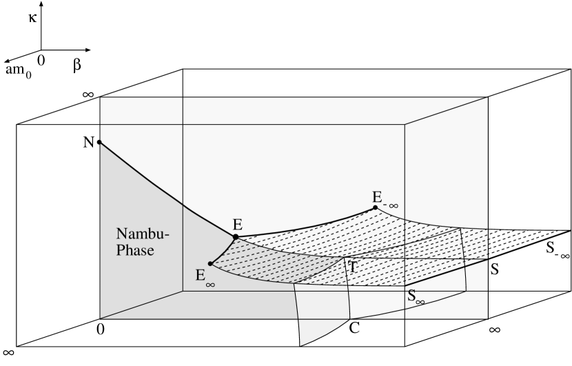
FIG. 1.: Schematic phase diagram of the $\chi U\phi$ model. Three critical lines, NE, E_∞E and E_-∞E meet at the tricritical point E. The line NE is a part of the boundary of the Nambu phase (dark shaded region) at $m_{0}=0$ with spontaneously broken chiral symmetry, $am_{F}\neq 0$. This phase is a sheet of first order phase transitions at which the chiral condensate changes sign. The lines E_∞E and E_-∞E are critical boundaries of the “wings” of first order Higgs phase transitions. The light shaded region at $m_{0}=0$ corresponds to vanishing fermion mass, $am_{F}=0$. The vertical sheets containing the points T and C separate the confinement and Coulomb phases. The line ETS is a line of tripple points.

1. Our previous studies [7, 8] have indicated that on the nearly whole chiral phase transition line, starting at the strong coupling limit $\beta=g^{-2}=0$, the model behaves like the Nambu–Jona-Lasinio (NJL) model, belonging presumably to the same universality class. We now present strong evidence that at $\beta=\beta_{E}\simeq 0.62$ the line contains a special point, the tricritical point E, where for theoretical reasons the scaling behavior is different from the rest of the line. It is governed by another fixed point. In difference to the NJL model the gauge field is not auxiliary but plays an important dynamical role at the point E.

2. Using advanced methods of the finite size scaling analysis we estimate several tricritical exponents determining the scaling behavior at the point E and find nonclassical values. This indicates that due to the strong gauge interaction this point differs from the standard expectations for tricritical points in four dimensions [9].

3. In the vicinity of the point E in the broken phase, not only the fermion mass $am_{F}$, but also the masses of several bosons (neutral states composed of scalar and gauge fields) and mesons ($\overline{\chi}\chi$ states) scale, i. e. in lattice units they approach zero with constant ratios. This suggests a rich spectrum if the continuum limit of the model is approached at the point E. In particular, a gauge ball of mass $m_{S}\simeq 1/2\,m_{F}$ is observed.

4. The composite Goldstone state $\pi$ with properties required by chiral symmetry breaking is present.

5. We determine the effective Yukawa coupling $y_{\rm R}$ between the composite $F$ and $\pi$ states in the vicinity of the critical line and find that lines of constant $y_{\rm R}$ tend to approach the point E [10]. We cannot yet say whether some of them end at this point, which would imply a nontrivial continuum limit. However, this approaching means that the coupling decreases only slowly with an increasing cutoff $1/a$ on paths towards E, thus increasing the chances for renormalizability.

We have not been able to achieve at least qualitative results in two issues of major interest: A heavy scalar $\sigma$-meson, which would correspond to a composite Higgs boson, is seen, but its mass in lattice units does not yet scale on the lattices of sizes we could afford and is strongly dependent on the bare fermion mass $am_{0}$. We cannot say anything about its value in the continuum limit at E. Also the pion decay constant $f_{\pi}$ does not scale, i.e. $f_{\pi}/m_{F}$ seems to increase with decreasing distance from E. Its current value (at $am_{0}\simeq 0.4$) is about 1/3. The present data are consistent both with the possibility that $f_{\pi}$ diverges in physical units, which would indicate triviality [11], and that the absence of scaling is due to too small lattices.

Concerning the possible triviality, we point out again [4] that the $\chi U\phi$ model would be a valuable model even if the cutoff cannot be removed completely without loosing the interaction, provided the cutoff dependence of the renormalized couplings is sufficiently weak, e.g. logarithmic as in the standard model. A dynamical approach to the Higgs-Yukawa mechanism does not necessarily require a nontrivial fixed point. The Higgs-Yukawa sector, whose validity is restricted due to the triviality by a certain upper energy bound, can be replaced by a theory with a higher upper bound.

Nevertheless, it is possible that the $\chi U\phi$ model in the continuum limit taken at the tricritical point E defines an interacting theory. The pursuit of this question requires a better understanding of tricritical points in four dimensions, as the available experience with such points is restricted to lower dimensions [9]. Further obstacles are the necessity to tune two couplings and the need to extrapolate to the chiral limit, $m_{0}\rightarrow 0$. Finally, more insight is needed into strongly coupled and not asymptotically free nontrivial four-dimensional gauge theories, whose existence has been recently suggested by numerical investigation of pure U(1) gauge theory [12].

We remark that the properties of the $\chi U\phi$ model in lower dimensions are much better accessible. In two dimensions, the numerical evidence strongly suggests that the continuum limit of the model is equivalent to the two-dimensional chiral Gross-Neveu model, and is thus renormalizable and asymptotically free [13]. First results in three dimensions [14] suggest that the $\chi U\phi$ model belongs to the universality class of the three-dimensional chiral Gross-Neveu model, which has a non-Gaussian fixed point. In both cases the continuum limit is obtained on a whole critical line of chiral phase transitions emerging from the corresponding Gross-Neveu model obtained in the limit of infinite gauge coupling, without any use of possible tricritical points. In this sense the situation in four dimensions is unique, and the experience from lower dimensions is not applicable.

If the tricritical point E in the four-dimensional $\chi U\phi$ model defines a renormalizable continuum theory, similar property might be expected in analogous models with other gauge symmetry groups. For example, an SU(2) gauge model with scalar and staggered fermion field in the fundamental representation of SU(2) is known to have at strong coupling a phase structure very similar to the $\chi U\phi$ model with the U(1) gauge field [5, 6]. Therefore we expect that the model we are studying is generic for a whole class of strongly coupled gauge models with fermions and scalars in the fundamental representation.

After describing the $\chi U\phi$ model in the next section, we present our results as follows: Some preparatory studies of the model in the limit of infinite bare fermion mass are presented in Section III. In the following section we demonstrate the existence of the tricritical point. In Section V the critical and tricritical exponents are estimated by finite size scaling studies. Spectrum in the continuum limit taken at the point E is discussed in Section VI. Then we summarize our results and conclude. In the Appendix we give a detailed definition of the meson propagators and effective Yukawa coupling we have calculated.

Preliminary results of this work have been presented in Refs. [15, 16]. An account of our results for the effective Yukawa coupling between $\pi$ and $F$ is given in a separate paper [10]. An investigation of the $\chi U\phi$ model in the quenched approximation, with particular emphasis on the role of magnetic monopoles, has been performed in Ref. [17]. A detailed presentation of the $\chi U\phi$ project in two, three, and four dimensions can be found in [18]. An investigation of similar models in continuum has been performed by Kondo [19].

II The $\chi U\phi$ model

A Action and phase diagram

The four-dimensional lattice $\chi U\phi$ model is defined by the action

$$S = S_{\chi}+S_{U}+S_{\phi},$$ (1)

$$S_{\chi} = \frac{1}{2}\sum_{x}\overline{\chi}_{x}\sum_{\mu=1}^{4}\eta_{x\mu}(U_{x,\mu}\chi_{x+\mu}-U^{\dagger}_{x-\mu,\mu}\chi_{x-\mu})$$ (3)

$$+{am_{0}}\sum_{x}\overline{\chi}_{x}\chi_{x},$$

$$S_{U} = -\beta\sum_{P}\cos(\Theta_{P}),$$ (4)

$$S_{\phi} = -{\kappa}\sum_{x}\sum_{\mu=1}^{4}(\phi^{\dagger}_{x}U_{x,\mu}\phi_{x+\mu}+h.c.).$$ (5)

Here $\Theta_{P}\in[0,2\pi)$ is the plaquette angle, i. e. the argument of the product of U(1) link variables $U_{x,\mu}$ along a plaquette $P$. Taking $\Theta_{P}=a^{2}gF_{\mu\nu}$, where $a$ is the lattice spacing, and $\beta=1/g^{2}$, one obtains for weak coupling $g$ the usual continuum gauge field action $S_{U}=\frac{1}{4}\int d^{4}xF_{\mu\nu}^{2}$. The staggered fermion field $\chi$ has (real) bare mass $am_{0}$ in lattice units and corresponds to four fermion species in the continuum limit. The scalar field $\phi$ is of fixed modulus, $|\phi|=1$.

The model has U(1) global chiral symmetry in the limit $m_{0}\rightarrow 0$, where $m_{0}$ is the bare fermion mass in physical units, to be defined while constructing the continuum limit. This is to be distinguished from the limit $am_{0}\rightarrow 0$, allowing explicit chiral symmetry breaking, $m_{0}\neq 0$, when $a\rightarrow 0$. Because of this fine difference between $m_{0}$ and $am_{0}$, important in various possible continuum limits, we keep trace of $a$ throughout the paper.

The schematic phase diagram is shown in Fig. 1. We recognize several limit cases of the $\chi U\phi$ model as models interesting by themselves:

1. At $\kappa=0$ and $am_{0}=\infty$, the pure U(1) gauge theory with the Wilson action (4) and phase transition between the confinement and Coulomb phases. Its continuum limit in an extended coupling parameter space may be determined by a non-Gaussian fixed point [12].

2. At $\kappa=0$ and $am_{0}$ finite, the gauge theory with fermions, i. e. compact QED (3) and (4), whose phase transition is currently under investigation [20].

3. At $\beta=0$, i.e. the gauge field being auxiliary, the Nambu–Jona-Lasinio (NJL) model, obtained by integrating out the bosonic fields [5]. The triviality of this model has been recently confirmed in large scale simulations [21, 11].

4. At $am_{0}=\infty$ and $\kappa$ arbitrary, the compact scalar QED or U(1) Higgs model (4) and (5). Its continuum limit at strong gauge coupling is Gaussian [22, 23].

At strong coupling, $\beta<1$, the model has three sheets of first order phase transitions: the two “wings” at finite $am_{0}$, and the sheet at $am_{0}=0$, separating the regions with nonzero chiral condensate of opposite sign. These three sheets have critical boundary lines E_±∞E and NE, respectively. As we shall discuss below, we have verified with solid numerical accuracy that these 2^nd order phase transition lines do indeed intersect at one point, the tricritical point E. We are not aware of a convincing theoretical argument why this should be so.

Of most interest is the Nambu phase at $m_{0}=0$, at small $\beta$ and $\kappa$. Because of confinement, there is no $\phi$-boson, i. e. charged scalar, neither fundamental charged $\chi$-fermion in the spectrum. The chiral symmetry is dynamically broken, which leads to the presence of the neutral composite physical fermion $F=\phi^{\dagger}\chi$ with the mass $am_{F}>0$. It scales, $am_{F}\searrow 0$, when the NE line is approached.

Further states include the “mesons”, i. e. the fermion-antifermion bound states: the Goldstone boson $\pi$ with $am_{\pi}\propto\sqrt{am_{0}}$, the scalar $\sigma$, and the vector $\rho$. “Bosons”, observed in the scalar-antiscalar or gauge ball channels are present too. It is in particular the neutral scalar boson $S$. In the vicinity of the E_±∞E lines the same scalar appears both in the $\phi^{\dagger}-\phi$ and gauge-ball channels which strongly mix. In the Nambu phase it is natural to interpret $S$ as a gauge ball, as this interpretation holds also deep in the Nambu phase, when the charged scalar $\phi$ is heavy.

The mass $am_{S}$ of the $S$-boson vanishes on the lines E_±∞E, whereas $am_{F}$ vanishes on the line NE. Both of them vanish at the tricritical point E. As their ratio is finite, the continuum limit obtained when approaching the point E contains both states and is thus different from the rest of the NE and E_±∞E lines.

The critical lines E_±∞E provide another approach to the continuum. For a nonvanishing $am_{0}$ the bare mass $m_{0}$ approaches then infinity and fermions decouple. The remaining U(1) Higgs model is equivalent to the trivial $\Phi^{4}$ theory at the critical endpoint of the Higgs phase transitions [22, 23]. This is confirmed by some of our results presented below.

B Observables and numerical simulations

For the investigation of the tricritical point we use the following observables:

To localize the Higgs phase transition we use the normalized plaquette and link energy are defined as

$$E_{\rm P} = \frac{1}{6V}\sum_{x,\,\mu<\nu}\mathop{\rm Re}\nolimits\{U_{x,\mu\nu}\}\;,$$ (6)

$$E_{\rm L} = \frac{1}{4V}\sum_{x,\nu}\mathop{\rm Re}\nolimits\{\phi_{x}^{\dagger}U_{x,\mu}\phi_{x+\mu}\}\;,$$ (7)

where V=$L^{3}T$ is the lattice volume. Following [23, 7] we use the perpendicular and parallel components of these energies,

$$E_{\perp} = E_{\rm L}\cos{\theta}+E_{\rm P}\sin{\theta}\;,$$ (8)

$$E_{||} = E_{\rm L}\sin{\theta}-E_{\rm P}\cos{\theta}\;,$$ (9)

where $\theta$ is the slope of the Higgs phase transition line at the endpoint in the plane ($\beta,4/3\kappa$).

For the localization of the chiral phase transition we measure the chiral condensate

$$\langle\overline{\chi}\chi\rangle=\left\langle\mathop{\rm Tr}\nolimits M^{-1}\right\rangle$$ (10)

via a stochastic estimator, where $M$ is the fermion matrix.

To calculate the mass of the physical fermion we consider the gauge invariant fermionic field $F_{x}=\phi^{\dagger}_{x}\chi_{x}$. The mass $am_{F}$ is measured by fitting its propagator in momentum space [7]. The results for the measurement in configuration space are consistent.

The fermion-antifermion composite states are called “mesons”. The corresponding operators and other details are given in [4, 18]. We tried to include also the annihilation part, but failed to obtain sufficient statistics.

To improve the signal, we also measure the meson propagators with smeared sources. This required the adaption of the routines, used with Wilson fermions, to the case of staggered fermions. It is described in Appendix A 1. With these smeared sources we have been able to fit the meson propagators by a one particle contribution at time distances larger than zero. But the same masses could be obtained if the unsmeared propagators were fitted with the inclusion of excited states. The smeared propagators reduce the errors, however, and in this work we mostly show results obtained by this method. Further details of the fitting procedure can be found in [18].

From the propagator of the $\pi$ meson also the pion decay constant $af_{\pi}$ can be calculated [24],

$$af_{\pi}=\sqrt{Z_{\pi}}\frac{am_{0}}{(am_{\pi})^{2}}\;.$$ (11)

Here $am_{\pi}$ and $Z_{\pi}$ are the mass and the wave function renormalization constant of the $\pi$ meson. We checked, that $af_{\pi}$ fulfills with excellent precision the current algebra relation

$$(af_{\pi}am_{\pi})^{2}=\frac{1}{2}am_{0}\langle\overline{\chi}\chi\rangle\;.$$ (12)

This is so even very close to the phase transition, though both $af_{\pi}$ and $\langle\overline{\chi}\chi\rangle$ show rather strong finite size effects there.

For the investigation of the chiral phase transition we also calculate the susceptibility ratio $R_{\pi}$, which is defined as the logarithmic derivative of the chiral condensate [25, 26],

$$R_{\pi}=\left.\frac{\partial\ln\langle\overline{\chi}\chi\rangle}{\partial\ln am_{0}}\right|_{\beta,\kappa}=\left.\frac{am_{0}}{\langle\overline{\chi}\chi\rangle}\frac{\partial\langle\overline{\chi}\chi\rangle}{\partial am_{0}}\right|_{\beta,\kappa}\;.$$ (13)

We measure it as the ratio of zero momentum meson propagators

$$R_{\pi}=\frac{C_{\sigma}(p=0)}{C_{\pi}(p=0)}$$ (14)

including the annihilation part of the propagator. This is done by means of a stochastic estimator and is described in detail in [18].

As explained in [25], we expect that close to a critical point the data could be described by means of the scaling law

$$R_{\pi}(t,am_{0})={\cal G}\left(\frac{am_{0}}{t^{\Delta}}\right),$$ (15)

where $t$ is the distance from the critical point (reduced coupling), $\Delta=\beta+\gamma$ the critical exponent and $\cal G$ a scaling function. At the critical point,

$$R_{\pi}(0,am_{0})={\cal G}(\infty)=\frac{1}{\delta}\,,$$ (16)

as can be seen by inserting $\langle\overline{\chi}\chi\rangle\propto(am_{0})^{1/\delta}$ into equation (13). At the critical point, $R_{\pi}$ should be independent of $am_{0}$ for sufficiently small $am_{0}$ (scaling region). In the broken phase, $R_{\pi}$ vanishes in the chiral limit, as can been seen easily from the definition. In the symmetric phase, the $\sigma$ and $\pi$ channels are degenerate, so that in the chiral limit $R_{\pi}=1$. For small fixed $t$ a characteristic behavior is expected, if one varies $am_{0}$: Because $\Delta>1$, close to the critical point the curves for $R_{\pi}$ start for $am_{0}=0$ from 0 and 1, respectively, and for increasing $am_{0}$ approach the horizontal line $1/\delta$. This will happen the faster the smaller $|t|$ is (compare fig. 12).

Further we consider the scalar and vector bosons, whose operators are defined as

$${\cal O}^{(S)}(t) = \frac{1}{L^{3}}\sum_{\vec{x}}\mathop{\rm Re}\nolimits\left\{\sum_{i=1}^{3}\phi^{\dagger}_{\vec{x},t}U_{(\vec{x},t),i}\phi_{\vec{x}+\vec{\imath},t}\right\},$$ (17)

$${\cal O}^{(V)}_{i}(t) = \frac{1}{L^{3}}\sum_{\vec{x}}\mathop{\rm Im}\nolimits\left\{\phi^{\dagger}_{\vec{x},t}U_{(\vec{x},t),i}\phi_{\vec{x}+\vec{\imath},t}\right\},$$ (19)

$$i=1,2,3.$$

The masses $am_{S}$ and $am_{V}$ of the scalar and vector bosons are calculated from the corresponding correlation functions in configuration space.

In the same way we also measure the gauge invariant combinations of the gauge fields, which we call gauge balls, in analogy to QCD glue balls. We define two operators with the quantum numbers $0^{++}$ and $1^{+-}$:

$${\cal O}^{(0^{++})}(t) = \frac{1}{L^{3}}\sum_{\vec{x}}\mathop{\rm Re}\nolimits\left\{\sum_{i=2}^{3}\sum_{j=1}^{i-1}U_{(\vec{x},t),ij}\right\},$$ (20)

$${\cal O}^{(1^{+-})}_{i}(t) = \frac{1}{L^{3}}\sum_{\vec{x}}\mathop{\rm Im}\nolimits\left\{U_{(\vec{x},t),jk}\big{|}_{i\neq j\neq k\neq i}\right\},$$ (22)

$$i=1,2,3.$$

The masses $am_{\text{G}}$ of the gauge-balls are calculated in analogy to the boson masses by means of the propagators in the configuration space.

We have observed mixing of the $S$ boson and the $0^{++}$ gauge ball by means of the two-point function

$$G^{(S,G)}(t)=\left\langle{\cal O}^{(S)}(0){\cal O}^{(0^{++})}(t)\right\rangle.$$ (23)

We have also measured the effective Yukawa coupling $y_{\text{R}}$ between the neutral fermion $F$ and the $\pi$ meson. This is done in analogy to [27], and the used operators are described in appendix A 2. A detailed discussion of our results is given in [10] and summarized in the conclusion of the present paper.

III Limit of infinite bare fermion mass

A U(1) Higgs model and chiral phase transition in the quenched approximation

For $am_{0}=\infty$, the $\chi U\phi$-model reduces to the U(1) Higgs model with $|\phi|=1$ on the lattice, (4) and (5). This model has been investigated in the eighties (for a review see e.g. [28]) and with modern methods in [22, 23]. Its phase diagram is represented by the front face of Fig. 1. It has the Coulomb phase at small $\kappa$ and large $\beta$, the rest being the confinement-Higgs phase. The line of Higgs phase transitions E_∞S_∞ is first order except the points E_∞ and S_∞. The continuum limit at the critical endpoint E_∞ corresponds most probably to a trivial scalar field theory [22, 23].

When dynamical fermions with $am_{0}>0$ are included, the phase diagram remains roughly the same, except that the confinement-Coulomb phase transition and the endpoint E${}_{am_{0}}$ shift to smaller $\beta$. The endpoints then form the critical line E_∞E. It is natural to expect that this line, except the tricritical point E, remains in the same universality class as the point E_∞. Our results confirm this expectation.

When quenched fermions with small $am_{0}$ are included into the Higgs model, a line of chiral phase transitions appears in the otherwise unchanged phase diagram of the Higgs model. It was realized already in the first investigations of the Higgs model with fermion, that full and quenched models have a very similar phase diagram [5, 6]. This includes the observation that the chiral phase transition line runs within numerical accuracy into the critical endpoint of the Higgs phase transition line. The phase diagram of the quenched model looks thus similar to the $am_{0}=0$ plane of Fig. 1.

This similarity suggests that it might be instructive to study the $\chi U\phi$-model in the quenched approximation. In Ref. [17] a quenched investigation of the interplay of chiral phase transition and the monopole percolation was performed. It seems that there might be an interplay of both transitions at an intermediate $\beta$ on the N_∞E_∞ line, possibly with nontrivial exponents. Around the points N_∞ and E_∞ the chiral and the percolation transitions appear to be separated, however.

B Scaling behavior at the endpoint E_∞

We begin by investigating the endpoint E_∞. We want to gain experience and check the reliability of the determination of critical exponents by means of Fisher zeros. We later apply this method at finite $am_{0}$ for the scaling investigation along the E_∞E line and compare the results with those at E_∞.

The scaling behavior at the endpoint of the Higgs phase transition line was determined in [22, 23] along the first order Higgs transition line. It was found that the endpoint is described by mean field exponents. We investigate the scaling behavior approaching $E_{\infty}$ in different directions. For this purpose it is useful to introduce the following reduced couplings (Fig. 2):

FIG. 2.: Definition of the reduced couplings $t$ and $h$ and of the angle $\theta$. The point E_∞ is the endpoint of the Higgs phase transition line. The scale of the $\kappa$ axis is 4/3 times larger than that of the $\beta$ axis.

$t$	:	parallel to the phase transition line of 1st order
$h$	:	perpendicular to the phase transition line.

Here perpendicular is understood in the same sense as in eqs.(8) and (9), so that

$$t = -(\beta-\beta_{c})\cos\theta+{\textstyle\frac{4}{3}}(\kappa-\kappa_{c})\sin\theta\,,$$ (24)

$$h = \phantom{-}(\beta-\beta_{c})\sin\theta\,+{\textstyle\frac{4}{3}}(\kappa-\kappa_{c})\cos\theta\,,$$ (25)

and therefore

$$S=-6V(tE_{||}+hE_{\perp})+S_{E_{\infty}}\;.$$ (26)

The letters $t$ and $h$ have been chosen in analogy to temperature and external field in magnetic systems.

We introduce critical exponents $\nu$ and $\tilde{\nu}$ of the correlation length for both directions,

$$\xi\propto|t|^{-\nu}|_{h=0}\,,$$ (27)

and

$$\xi\propto|h|^{-\tilde{\nu}}|_{t=0}\,,$$ (28)

$\xi$ being the correlation length diverging at E_∞.

To understand the relation between $\nu$ and $\tilde{\nu}$ we assume the equation of state

$$\xi=|t|^{-\nu}F\left(\frac{|h|}{|t|^{\Delta}}\right)\;,$$ (29)

with the scaling function $F$ and $\Delta=\beta+\gamma$. Introducing $\tilde{F}(x)=x^{\nu}F(x^{\Delta})$ it can be rewritten as

$$\xi=|h|^{-\nu/\Delta}\tilde{F}\left(\frac{|h|^{1/\Delta}}{|t|}\right)\;.$$ (30)

Assuming $\tilde{F}(\infty)<\infty$ this means $\tilde{\nu}=\nu/\Delta$.

The scaling behavior (28) is expected in the general direction $t=c\cdot h$, because $\Delta>1$, and therefore

$$\frac{|h|^{1/\Delta}}{|t|}=h^{1/\Delta-1}/c\rightarrow\infty$$ (31)

for $h\rightarrow 0$ and, accordingly, $t\rightarrow 0$. This makes clear that it is not important to choose $h$ perpendicular to $t$. Only the $t$-direction ($h=0$) is special as it is tangential to the phase transition line and thus described by the scaling law (27).

The mean field values of the exponents $\beta=1/2$, $\gamma=1$, and $\nu=1/2$ correspond to $\tilde{\nu}=1/3$.

To determine the critical exponent of the correlation length we measure the scaling behavior of the edge singularity in the complex coupling plane (Fisher zero)[29]. From scaling arguments for the free energy we expect for the first zero $z_{1}$:

$$\left.\mathop{\rm Im}\nolimits z_{1}(L)\right|_{t=0}=A\cdot L^{-1/\tilde{\nu}}\;.$$ (32)

As all directions which are not tangential to the phase transition line are equivalent, we expect the same exponent $\tilde{\nu}$ also if we fix $\beta=\beta_{\rm E_{\infty}}$ or $\kappa=\kappa_{\rm E_{\infty}}$. This was verified in [15]. Fixing one of the couplings is particularly convenient for the necessary analytic extrapolations into the complex plane. That is done by means of the multihistogram reweighting method [30].

We present here the scaling investigation we did for $\beta=0.848\approx\beta_{\rm E_{\infty}}$. Fig. 3a shows a nice scaling behavior for all lattice sizes with the critical exponent $\tilde{\nu}=0.3236(10)$. This value is very close the mean field exponent $\tilde{\nu}=1/3$.

(a)

(b)

FIG. 3.: (a) Scaling behavior of the edge singularity for $\beta=0.848\simeq\beta_{\text{E}_{\infty}}$ in the U(1) Higgs model on $L^{4}$ lattices. The small deviations from the trivial scaling behavior with $\tilde{\nu}=1/3$ are resolved in (b). Here $\ln(L^{3}\mathop{\rm Im}\nolimits z_{1})$ is shown as a function of $\ln(\ln L)$. The fit from Fig. (a) is shown dotted. The value for $\beta_{\text{E}_{\infty}}$ has been taken from [23].

The small deviations outside the error bars are probably due to logarithmic corrections, as they are expected at Gaussian fixed points. To verify this we follow the idea from [31] and factor out the leading power law $L^{-1/\tilde{\nu}}$. If the scaling behavior has the form

$$L^{3}\left.\mathop{\rm Im}\nolimits z_{1}(L)\right|_{t=0}=A\cdot(\ln L)^{-p}\;,$$ (33)

we expect in the $\ln\ln$ plot a strait line with the slope $-p$. The data shown in Fig. 3b are very well described by a straight line with $p\simeq 0.17$. The $\chi^{2}$ is smaller than that with a fit by means of the equation (32). However, we have not investigated how far these results, and especially $p$ depend on the precise knowledge of the critical point.

A similar value for the exponent $\tilde{\nu}$ was also measured in the SU(2) Higgs model [32, 33], but then it was not realized that this value is actually compatible with a Gaussian fixed point. Now we can conclude that the U(1) and SU(2) Higgs models have a very similar scaling behavior at the endpoint.

We have also determined the critical exponent $\tilde{\nu}$ by means of the finite size scaling of the specific heat and of some cumulants [18]. These less precise methods confirm the results presented here. Also the shift exponent $\lambda$ has turned out to be compatible with $1/\tilde{\nu}$ for the investigated observables [15, 18].

IV Existence and position of the tricritical point $E$

A General properties of tricritical points

To present our investigations of the tricritical point E, we first summarize the relevant general properties of tricritical points and define the exponents. In notation we follow Griffiths [34].

In the vicinity of a tricritical point it is usual to choose the following orthogonal coordinate system (Fig. 4):
$\lambda$ : tangential to the first order PT line in the symmetry plane, $g$ : perpendicular to the PT line inside the symmetry plane, $\zeta$ : perpendicular to the symmetry plane.
In the symmetry plane $m_{0}=0$, these definitions are analogous to those in the Higgs model (sec. III B), $\lambda$ and $g$ corresponding to $t$ and $h$, respectively.

In the phase diagram there are four special lines, which we denote following [9]: the chiral PT line NE (second order) in the symmetry plane ($\lambda>0$) is lambda line L_λ, its continuation in the symmetry plane, on which three first order phase transition sheets meet ($\lambda<0$), is triple line L_τ, and the two lines of endpoints outside the symmetry plane are wing critical lines L₊ and L_-. The first order PT plane below the lines L_λ and L_τ in the symmetry plane is denoted S₀, and the two wings of Higgs phase transitions are S₊ and S_-. Because of the $\pm am_{0}$ symmetry we use in the following only the index $+$.

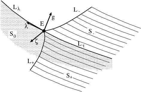
FIG. 4.: Schematic phase diagram of the first order PT planes and the critical lines (L_±, L_λ) in the vicinity of the tricritical point E. L_τ is the line of triple points. The L lines correspond the lines in Fig. 1 as follows: L${}_{\lambda}\,\hat{=}\,\mbox{NE}$, L${}_{\pm}\,\hat{=}\,\mbox{E${}_{\pm\infty}$E}$, L${}_{\tau}\,\hat{=}\,\mbox{ET}$. A local coordinate system is shown.

exp.	[9]	definition	class.
			value
$\alpha_{t}$	$\alpha_{t}$	$\frac{\partial E_{\perp}}{\partial g}\propto g^{-\alpha_{t}}$, $\lambda=\zeta=0$	$\frac{1}{2}$
$\alpha_{u}$	$\alpha$	$\frac{\partial E_{||}}{\partial\lambda}\propto\lambda^{-\alpha_{u}}$, $g=\zeta=0$	-1
$\beta_{t}$	$\beta_{t}$	$\langle\overline{\chi}\chi\rangle\propto|g|^{\beta_{t}}$, $\lambda=\zeta=0$	$\frac{1}{4}$
$\beta_{u}$	$\beta_{2}$	$\Delta E_{\perp}\propto|\lambda|^{\beta_{u}}$, $g=\zeta=0$, $\lambda<0$	1
$\delta_{t}$	$\delta$	$\langle\overline{\chi}\chi\rangle\propto\zeta^{1/\delta_{t}}$, $\lambda=g=0$	5
$\delta_{u}$	$1/\beta_{2t}$	$|E_{\perp}-E_{\perp c}|\propto|g|^{1/\delta_{u}}$, $\lambda=\zeta=0$	2
$\nu_{u}$		$\xi_{+}\propto|\lambda|^{-\nu_{u}}$, $g=\zeta=0$	1
$\tilde{\nu}_{u}$		$\xi_{+}\propto|g|^{-\tilde{\nu}_{u}}$, $\lambda=\zeta=0$	$\frac{1}{2}$
$\nu_{t}$		$\xi_{\lambda}\propto|g|^{-\nu_{t}}$, $\lambda=\zeta=0$	$\frac{1}{2}$
$\phi$	$\phi$	$g\propto|\lambda|^{\phi}$ at the lines Lλ and Lτ, $\zeta=0$	2
$\phi\Delta_{t}$	$\Delta$	$\zeta\propto|\lambda|^{\phi\Delta_{t}}$ at the lines L+	$\frac{5}{2}$
$\Delta_{u}$		$\Delta_{u}=\beta_{u}\delta_{u}$	2

TABLE I.: Exponents at the tricritical point. In the second column the notation of [9] is given. The classical value is derived in three dimensions. Its applicability to four dimensions is discussed in the text.

The most important exponents and the defining scaling behavior are summarized in table I. Comparing a metamagnet to our model, the staggered magnetization corresponds to the chiral condensate and the magnetization to the energy $E_{\perp}$. The unfortunate fact is that the symmetry plane, which is of major use in the study of metamagnets, corresponds to the chiral limit $m_{0}=0$, which is difficult to approach in numerical simulations with fermions coupled to a gauge field.

The two sets of exponents with index $t$ and $u$ are defined in analogy to the exponents on the adjacent critical lines: The set with the index $t$ (tricritical exponents) is defined in analogy to the exponents along the chiral PT line NE (L_λ line). The set with the index $u$ (subsidiary exponents) is defined in analogy to the exponents along the line of Higgs endpoints E_∞E (L₊ line). In general, the exponents at the tricritical point are different from those at the adjacent lines. We denote the diverging correlation lengths and the exponents on the lines L_λ and L₊ by the indices $\lambda$ and $+$, respectively.

The tricritical point can be considered as a special point of both the L_λ and the L₊ critical lines. Both the correlation length $\xi_{\lambda}$ diverging at the L_λ line and the correlation length $\xi_{+}$ diverging at the L₊ line are critical there. Nevertheless, in general, $\xi_{\lambda}$ and $\xi_{+}$ are to be distinguished also at the tricritical point. In our case $\xi_{\lambda}=1/am_{F}$ and $\xi_{+}=1/am_{S}$.

Our results strongly indicate (sec. VI A 2), that at the point E, $\xi_{\lambda}\propto\xi_{+}$ on all paths into the point E. This proportionality seems to hold also for all other observed correlation lengths (inverse masses) which diverge at the point E. Thus there seems to be only one scaling law and $\tilde{\nu}_{u}=\nu_{t}$. This is a generic property of tricritical points. It makes possible to use at the tricritical point the finite size scaling theory quite in analogy to the adjacent critical lines.

In three dimensions it is usual that tricritical points have a large region of dominance. In analogy, near the tricritical point we expect to find at some distance from the second order PT lines already the scaling behavior described by the tricritical exponents. Such a crossover phenomenon was investigated for example in [35]. A similar effect might be expected also on small lattices in the immediate vicinity to the PT lines. It is not excluded, however, that in four dimensions the tricritical points are much less dominant than in three-dimensional models. To the best of our knowledge, tricritical points have not yet been investigated numerically in four dimensions.

For the singular part of the free energy $F$ usually the following scaling relations are assumed [9]:

$$F_{\rm sing}(\lambda,g,\zeta) = |\lambda|^{2-\alpha_{u}}{\cal F}^{(\pm)}\left(\frac{g}{|\lambda|^{\phi}},\frac{\zeta}{|\lambda|^{\phi\Delta_{t}}}\right),$$ (34)

$$F_{\rm sing}(\lambda,g,\zeta) = |g|^{2-\alpha_{t}}{\cal F}_{1}^{(\pm)}\left(\frac{\lambda}{|g|^{1/\phi}},\frac{\zeta}{|g|^{\Delta_{t}}}\right)\;.$$ (35)

For such systems several relations between the exponents can be derived [34]:

$$\alpha_{t} = 1-1/\delta_{u}\,,$$ (36)

$$\Delta_{u} = \phi\,,$$ (37)

$$2-\alpha_{u} = \phi(2-\alpha_{t})\,,$$ (38)

$$\nu_{u} = \phi\nu_{t}$$ (39)

$$1+\delta_{t} = (2-\alpha_{t})/\beta_{t}\,,$$ (40)

$$\Delta_{t} = \beta_{t}\delta_{t}=(2-\alpha_{u})/\phi\cdot\delta_{t}/(1+\delta_{t})\,,$$ (41)

$$\beta_{t} = (2-\alpha_{t})/(1+\delta_{t})\,.$$ (42)

In our work we use in particular the last two of these relations.

Only four exponents are independent. With the assumption that the hyperscaling relation

$$\alpha_{t}=2-d\nu_{t}$$ (43)

holds, only three independent exponents remain.

Unfortunately, theory of tricritical points in four dimensions is developed only insufficiently. The Ginzburg criterion indicates that for all dimensions $d\geq 3$, tricritical point can be described by the classical exponents. This would correspond in four dimensions to a violation of the hyperscaling relation [9].

B Two diverging correlation lengths

For the existence of the tricritical point E in the $\chi U\phi$ model the chiral and Higgs phase transition must meet at one point in the $m_{0}=0$ plane. Since there is no theoretical understanding for the interplay between both transition, the existence of such a point has to be demonstrated numerically.

To give a first impression, Fig. 6 shows the mass of the scalar boson $am_{S}$ in the vicinity of the tricritical point for $am_{0}=0.01$, 0.02, and 0.04. This mass has been obtained from the $\phi^{\dagger}-\phi$ correlation function (17). It has a pronounced minimum (arrows in Fig. 6) for each $am_{0}$. Its minimal value on the $6^{3}16$ lattice is about 0.35, and 0.2 on the $8^{3}24$ lattice. The significant decrease with increasing lattice size indicates that the mass in the infinite volume vanishes, and the correlation length $\xi_{+}=1/am_{S}$ thus diverges. The vanishing of $am_{S}$ at some $\beta$, $\kappa$ for any finite $am_{0}$ corresponds to the E_∞E line of endpoints E${}_{am_{0}}$ of the Higgs phase transitions.

FIG. 5.: Boson mass $am_{S}$ as function of $\beta$ for different $am_{0}$ and lattice sizes at $\kappa=0.30\approx\kappa_{\rm E}$. The arrows indicate the minima of $am_{S}$.

FIG. 6.: Fermion mass $am_{F}$ as function of $\beta$ for different $am_{0}$ and lattice sizes at $\kappa=0.30$. The minima of the boson mass $am_{S}$ are marked with full symbols and arrows (cf. Fig. 6).

The fermion mass $am_{F}$ descends steeply (Fig. 6) at the position of the minimum of the boson mass for the same $am_{0}$ and volume. In the broken phase, the curves for different volumes slowly approach each other. In the symmetric phase, the values of $am_{F}$ achieve small finite values which should vanish in the chiral limit and infinite volume.

Figures 6 and 6 show that changes of volume and $am_{0}$ result in a shift of the minimum in $\beta$. The same holds for $\kappa$. So there is little hope to extrapolate the data at fixed $\beta$ and $\kappa$ into infinite volume and chiral limit. As usual for tricritical points, a fine tuning of both couplings is required. In this work we assume that the limited precision of the position of the tricritical point we have achieved is outweighted by a sufficiently large domain of dominance of this point.

C Position of the tricritical point E

To localize the point E we determine the positions of the endpoints E${}_{am_{0}}$ for small $am_{0}$ and extrapolate them to $am_{0}=0$. It is difficult to control the uncertainties in every step of this procedure.

At nonzero $am_{0}$ we proceed in analogy to [23]. We determine the latent heat of $E_{\perp}$ in the S₊ plane. Fig. 7 shows the latent heat $\Delta E_{\perp}$ as a function of $\beta$ for two $am_{0}$ and different lattice sizes. The values have been obtained by reweighting the data to the coupling where both maxima have the same height. Then the distance of these maxima in the histogram and the uncertainty have been estimated, as the data is not sufficient for a fitting procedure.

FIG. 7.: Square of the latent heat of the energy $E_{\perp}$ for $am_{0}=0.02$ and $am_{0}=0.04$ for lattices of the size $4^{4}$ to $8^{4}$ and $10^{4}$, resp.. The mean-field exponent $\beta_{+}=\frac{1}{2}$ corresponds to a strait line. We have described the data for each $am_{0}$ with one common $\beta_{+}$ in eq. (44) for the different lattice sizes.

We expect a scaling of $\Delta E_{\perp}$ for fixed $am_{0}$ and fixed lattice size of the form

$$\Delta E_{\perp}\propto t^{\beta_{+}}\propto\left(\beta-\beta_{pc}(L,am_{0})\right)^{\beta_{+}}\;.$$ (44)

The index $+$ denotes the magnetic exponent on the E_∞E line. In this procedure it is assumed that the dominant contribution due to the finite volume can be absorbed in a volume dependent pseudocritical coupling $\beta_{pc}(L,am_{0})$. A better method would have been to extrapolate the latent heat first into the infinite volume and to investigate scaling afterwards. But for such an analysis the quality of our data is not sufficient.

In the quadratic plot in Fig. 7 we expect a straight line for the classical value $\beta_{+}=\frac{1}{2}$, which was observed for $am_{0}=\infty$ [23]. Our data at small $am_{0}$ are well compatible with this expectation.

A fit with free $\beta_{+}$ gives a value of $\beta_{+}=0.5(3)$ for $am_{0}=0.04$, and $\beta_{+}=0.5(4)$ for $am_{0}=0.02$. The probably overestimated error for $\Delta E_{\perp}$ results in an overestimated error of $\beta_{+}$. In fact our data do not have the necessary quality to investigate the scaling (44) with a free exponent $\beta_{+}$. Therefore, we fit them with fixed $\beta_{+}=0.5$. For $\beta_{pc}(L,am_{0})$ obtained in this way we assume scaling as in the Higgs model [23] with $\nu_{+}=0.5$:

$$\beta_{pc}(L,am_{0})-\beta_{c}(am_{0})\propto L^{-1/\nu_{+}}\;.$$ (45)

Our data are compatible with this assumption (Fig. 8).

FIG. 8.: Pseudocritical couplings $\beta_{pc}(L)$ as function of $L^{-2}$ for different $am_{0}\leq 0.10$. The fit is an extrapolation into infinite volume assuming the exponent value $\nu_{+}=0.5$.

The so determined points $\beta_{c}(am_{0})$ of the E_∞E line are listed in table II and plotted in Fig. 9. The point at $am_{0}=1.00$ was only estimated and the uncertainty included in error bars [18].

$am_{0}$	$\beta_{c}$	$\kappa_{c}$
0.02	0.654(7)	0.304(5)
0.04	0.671(4)	0.296(4)
0.06	0.684(4)	0.292(3)
0.10	0.707(3)	0.285(3)
1.00	0.80(2)	0.28(1)
$\infty$	0.848(4)	0.263(2)

TABLE II.: Estimate for the position of the critical endpoints E${}_{am_{0}}$ on the E_∞E line (L₊) in the infinite volume limit.

FIG. 9.: Projection of the critical line of endpoints E_∞E and the line of triple-points TT_∞ onto the $\beta$-$am_{0}$-plane. (In Fig. 1 this corresponds to a view from below for $am_{0}\geq 0$.) Shown is also the critical line NE of chiral phase transitions. The points have been determined on $6^{4}$ and $8^{4}$ lattices. The error bars reflect the uncertainty of the extrapolation into the infinite volume.

FIG. 10.: The values of $\beta_{c}(am_{0})$ for $am_{0}\leq 0.10$ obtained from extrapolation into infinite volume by means of (45). The fit shows their extrapolation into the chiral limit using (46).

These results for $\beta_{c}(am_{0})$ are extrapolated into the chiral limit. The curves should approach the symmetry plane with the critical exponent $\phi\Delta_{t}$:

$$\beta_{c}(am_{0})-\beta_{c}(E)\propto\lambda_{c}(am_{0})\propto(am_{0})^{\phi\Delta_{t}}$$ (46)

A fit of the data obtained for $am_{0}\leq 0.10$ gives $\phi\Delta_{t}\approx 1.6$ (Fig. 10). This value is in agreement with that obtained by means of the relation (41) from the values of the exponents determined in the next section. There we find $\phi\Delta_{t}=1.8(1)$. The extrapolated $\beta$ value for the point E is $\beta_{\rm E}\simeq 0.625$. Of course, with three free parameters used to fit four data points the error is large and uncertain.

The satisfactory quality of the fit and the agreement of both methods for the determination of $\phi\Delta_{t}$ indicates, that we may actually overestimate the errors in the whole procedure. E.g. fixing $\phi\Delta_{t}=1.8$ in eq. (46) reduces the error for $\beta_{\rm E}$ without reducing the quality of the fit shown in Fig. 10 and gives $\beta_{\rm E}=0.62(1)$.

In summary, we estimate the coordinates for the point E in infinite volume to be:

$$\beta_{\rm E} = 0.62(3)\;,$$ (47)

$$\kappa_{\rm E} = 0.32(2)\;.$$ (48)

The rather small improvement of the precision compared to our earlier publication [7] shows how difficult the determination of the position of the tricritical point is, if no simulations in the symmetry plane are possible. Nevertheless, our present determination is much more reliable due to the use of the scaling analysis.

V Critical and tricritical exponents

A Exponents $\nu_{t}$ and $\beta_{u}$

We have seen in section III B that the scaling behavior at the point E_∞ is mean-field-like. We now repeat the analysis by means of Fisher zeros also for small fixed $am_{0}$ and determine $\tilde{\nu}_{am_{0}}$, the value of $\tilde{\nu}$ at fixed $am_{0}$, pursuing two aims. We want to check the universality along the E_∞E line, and we want to look for a possibly different scaling behavior in the immediate vicinity of the tricritical point E.

To use the method of the Fisher zeros, one coupling has to be fixed. For each $am_{0}$ we have fixed $\beta$ at the position of ${\rm E}_{am_{0}}$. At this $\beta$ we have done simulations for different $\kappa$ and afterwards determined the zeros in the complex $\kappa$ plane. The accuracy of the method is limited by the uncertain precision of $\beta_{c}(am_{0})$, as given in table  II. To estimate this dependence, we have made measurements at three $\beta$-values for $am_{0}=0.02$. Between 9600 and 64000 HMC-Trajectories have been done for each $\beta$ value at 5-7 $\kappa$-points.

FIG. 11.: Scaling behavior of the edge singularity: (a) for $am_{0}=0.04$ and $\beta=0.67$, (b) for $am_{0}=0.02$ and $\beta=0.64$, 0.655, 0.66 on quadratic lattices. $\beta=0.67$ is our current best estimate for the position of the endpoint ${\rm E}_{am_{0}}$ at $am_{0}=0.04$. For $am_{0}=0.02$ we have investigated three different $\beta$ values, $\beta=0.655$ is nearest to the endpoint.

Fig. 11 shows the scaling behavior of the imaginary part of the Fisher zero in $\kappa$ for $am_{0}=0.04$ and $0.02$. In all cases, no deviations from a linear behavior could be observed. The value $\tilde{\nu}_{+}=\tilde{\nu}_{0.04}=0.328(4)$ for $am_{0}=0.04$ is in excellent agreement with the result at $am_{0}=\infty$. For $am_{0}=0.02$ it was more difficult to find the critical coupling $\beta_{c}(0.02)$. From the three measurements we estimate $\tilde{\nu}_{0.02}=0.33(4)$.

Investigation of the cumulants yields results for $\tilde{\alpha}_{+}/\tilde{\nu}_{+}$ which are consistent with the use of the Josephson relation. This indicates that the hyperscaling hypothesis is fulfilled. The calculation of $\tilde{\nu}_{+}$ with use of the Josephson relation yield consistent results with a little bit larger error.

The finite size scaling theory above the critical dimension should be applied with care. It is possible that in spite of consistent scaling it is not the exponent $\nu$ which is observed. In our case the values of $\tilde{\nu}_{+}$ obtained by this method and from the scaling of the fermion mass are consistent, however.

Therefore, we interpret our results as a good confirmation of the universality along the E_∞E line. The measured values are nearly identical to those at $am_{0}=\infty$. Also the logarithmic corrections seem to tend into the same direction. Since we found similar results also for $\beta_{+}$ it is likely that all exponents along the E_∞E line are independent of $am_{0}$.

Assuming that for the small values of $am_{0}$, we could investigate, the dominance region of the tricritical point is already achieved, we expect that for $am_{0}\rightarrow 0$ the exponent $\tilde{\nu}_{+}$ turns over into $\tilde{\nu}_{u}=\nu_{t}$. This implies that the subsidiary exponents with the index $u$ are identical or at least very similar to the exponents along the E_∞E line, which are the corresponding classical values. The measured value then corresponds to $\nu_{t}=\frac{1}{3}$. This means, that the value is different from the classical values of a tricritical point. The corresponding classical prediction $\nu_{t}=\frac{1}{2}$ is hardly compatible with the data.

A crossover to the exponents of the tricritical point at small $am_{0}$ could be expected also for the exponent $\beta_{+}$, which we measured along the E_∞E line (in the S₊ plane) in section IV C. However, also here we could not observe any $am_{0}$ dependence and $\beta_{+}$ is compatible with the mean field exponent of a critical line $\beta_{+}=\frac{1}{2}$ down to $am_{0}=0.02$. We therefore interpreted this results as a indication, that also $\beta_{u}$ is close to $\frac{1}{2}$.

B Estimate of $\delta_{t}$ from $R_{\pi}$

As suggested in [25] it is possible to determine the ‘magnetic’ exponent $\delta$ for fermionic theories by measuring the susceptibility ratio $R_{\pi}$ for different small $am_{0}$ around the critical point. We have measured $R_{\pi}$ for different $\kappa$ values. Inside the broken phase ($\kappa<\kappa_{c}$), we expect a curve which approaches $R_{\pi}=0$ for $am_{0}\rightarrow 0$. In the symmetric phase ($\kappa>\kappa_{c}$), we expect the curve to approach $R_{\pi}=1$ for $am_{0}\rightarrow 0$. At the critical point ($\kappa=\kappa_{c}$), the line should be horizontal for small $am_{0}$ and the corresponding value of $R_{\pi}$ is equal to $1/\delta=1/\delta_{t}$.

We have tried this method in our model at $\beta=0.55$ on the NE line (Fig. 12). For $\kappa=0.37$ the curves bend downward when approaching the chiral limit, for $\kappa=0.38$ they bend upward. This indicates, that the critical $\kappa$ is between 0.37 and 0.38, in agreement with 0.376(5), our estimate based on the modified gap equation [7]. The estimated horizontal line separating both phases is at $R_{\pi}=0.30(5)$. This is in good agreement with the mean field value of $\delta=1/R_{\pi}=3$. Both results confirm our earlier result that the phase transtion at $\beta=0.55$ is mean-field-like [7].

FIG. 12.: $R_{\pi}$ as function of $am_{0}$ at $\beta=0.55$ on $6^{4}$, $8^{4}$ and $10^{4}$-lattices for different $\kappa$.

FIG. 13.: $R_{\pi}$ as function of $am_{0}$ close to the tricritical point at $\beta=0.64$ on $8^{4}$ and $10^{4}$-lattices for different $\kappa$.

Our results for $\beta=0.64$, close to the tricritical point, are shown in Fig. 13. A horizontal curve is found for $\kappa_{c}=0.307(2)$. It extrapolates to $R_{\pi}(\kappa_{c})=0.10(5)$. We estimate that $\delta_{t}=10^{+10}_{-4}$ under the assumption, that the increase of the volume does not change this picture significantly. Indeed, the data for the $8^{4}$ and $10^{4}$ differ only very little.

To estimate the sensitivity of these results on $\beta$ we have obtained lower statistics data also at $\beta=0.62$, our current best estimate for $\beta_{\rm E}$. The results are very similar to those at $\beta=0.64$. This indicates that for $\beta=0.64$ we are already in the influence region of the tricritical point.

Also an explorative investigation with the method of the Lee-Yang zeros in the complex $am_{0}$ plane, as we applied recently in the three-dimensional model [36, 14], confirms the large value for $\delta_{t}$. Using the lattices $4^{4}$ and $6^{4}$ we get for $\beta=0.64$ and $\kappa=0.307$ the estimate $\tilde{\nu}\simeq 0.275$, which corresponds to $\delta_{t}=10$.

C Summary of results for the tricritical exponents

We have determined three independent exponents at the tricritical point:

$$\nu_{t} = 0.33(5),$$ (49)

$$\beta_{u} = 0.5(2),$$ (50)

$$\delta_{t} = 10^{+10}_{-4}\,.$$ (51)

These values disagree with the classical values for tricritical points expected in four dimensions, $\nu_{t}=0.5$, $\beta_{u}=1$, $\delta_{t}=5$.

The errors take into account only uncertainties in the measurement. We cannot estimate possible systematic errors. In particular we have assumed that at $am_{0}=0.02$ on the used lattices we observe the asymptotic scaling behavior of the tricritical point. Some support for this assumption is obtained in the spectrum analysis in the next section. It is plausible also because typically tricritical points have a large region of influence and the corresponding deviations from the scaling behavior are small.

If one assumes the validity of the scaling laws, all further exponents are fixed. We only could check with good precision the Josephson relation between $\alpha_{t}$ and $\nu_{t}$. Some very crude check was possible for $\nu_{u}$, and another one for $\beta_{t}$ is described in Sec. VI A 4. We found no indications for a violation of the scaling laws.

VI Spectrum

To analyze the possible physical content of the continuum limit taken at the point E, it is important to study the spectrum. This investigation has the advantage that it is relatively independent of the missing theory of tricritical points in four dimensions. Here we give only the most important results. A tabular overview of the measured values (which could be presented even graphically only in part) can be obtained from the authors.

Most of the shown results have been obtained for fixed $\kappa=0.30$. The reason for this is the observation, that the shift of the endpoint E${}_{am_{0}}$ with $am_{0}$ is smaller in the $\kappa$ direction than in the $\beta$ direction. The advantage of this is, that for different $am_{0}$ the endpoint E${}_{am_{0}}$ can be approximately hit with one $\kappa$. The difference of this chosen value of $\kappa$ from our current best estimate $\kappa_{\rm E}=0.32(2)$ is due to the underestimated remaining shift at the beginning of the large scale simulation. The value $\kappa=0.30$ corresponds the the position of the endpoint E${}_{am_{0}}$ at $am_{0}\approx 0.03$.

Some measurements with less statistics have been performed for $\beta=0.64$ and $\kappa=0.305$. They confirm the picture presented here. In particular, they indicate a common scaling behavior in a whole region around E, e.g. independent of the direction of approach to this point, provided it is not tangential to the critical lines.

A Fermion, boson and gauge-ball spectrum

1 Uniform behavior as a function of $am_{F}$

The pictures showing the behavior of the mass of fermion and scalar boson S in the vicinity of E have been shown already in section IV B. The very similar position of the pseudocritical area of $am_{S}$ and $am_{F}$ for different volumes and small $am_{0}$ for $\kappa=0.30\simeq\kappa_{\rm E}$ suggests to express one mass as a function of the other.

As $am_{F}$ is monotonously decreasing with increasing $\kappa$ or $\beta$, and is well measurable, we plot $am_{S}$ as a function of $am_{F}$ (fig. 14). In this figure the broken phase is to the right and the symmetric phase to the left. The border between both phases is at the minimum of the boson mass. In the infinite volume and the chiral limit, the symmetric phase would reduce in this plot to one point, $am_{F}=0$. This kind of plot as a function of $am_{F}$ is possible for all couplings near to the NE line, but $am_{S}$ scales only at the point E.

FIG. 14.: Boson mass $am_{S}$ as function of the fermion mass $am_{F}$. The broken phase is to the right from the minima.

To extract continuum physics in this way, it is necessary to check that all curves are close to a uniform curve, when the tricritical point is approached. In principle, this means the fourfold limit $V\rightarrow\infty$, $am_{0}\rightarrow 0$, $\kappa\rightarrow\kappa_{\rm E}$ and $\beta\rightarrow\beta_{\rm E}$.

One can see that in the broken phase, $am_{S}$ as a function of $am_{F}$ is nearly independent of volume and $am_{0}$. For other $\kappa\simeq\kappa_{\rm E}$ and $\beta\simeq\beta_{\rm E}$ nearly the same curves result. From this nontrivial observation we conclude, that our data for fixed $am_{0}$ and $\kappa=0.30$ correspond approximately to a path towards E for $am_{0}=0$. For small $am_{F}$, at the transition into the symmetric phase, the boson mass $am_{S}$ increases rapidly. As expected, the minimum shifts to the left for increasing lattice size and decreasing $am_{0}$, which corresponds to the approach to the critical theory (chiral limit in the infinite volume).

In the following, all observables are plotted as a function of $am_{F}$. To make the figures more clear, usually only the data on the $8^{3}24$ lattice are shown, as long as the effects of finite volume in this kind of plot are small.

2 Scaling behavior of $am_{S}$

To investigate the scaling behavior of $am_{S}$ we look at the mass ratio $m_{S}/m_{F}$. As shown in fig. 15, this ratio is nearly constant, and close to 0.5 in the broken phase. A small decrease of this ratio for decreasing $am_{F}$ is indicated. Most probably the reason for this is, that for nonzero $am_{0}$, the boson mass $am_{S}$ vanishes at the point E${}_{am_{0}}$ in the $V\rightarrow\infty$ limit, whereas $am_{F}$ stays finite. We have checked that approximately the same mass ratio is obtained also on other paths into the point E. This strongly suggests that this mass ratios is preserved also in the continuum limit. This would mean that the scalar boson would survive with approximately half the fermion mass.

FIG. 15.: Mass ratio $m_{S}/m_{F}$ as function of the fermion mass.

This similar scaling behavior means, that both observables have a common critical point. This is our strongest argument for the coincidence of chiral and Higgs phase transition at the point E which is thus a tricritical point.

The fact that this nice scaling behavior can be observed for all investigated $am_{0}\leq 0.04$ further suggests that these values of the bare mass are inside the dominance region of the tricritical point. In the influence region of the E_∞E critical line $am_{F}$ would stay finite whereas $am_{S}$ would scale to zero. This should at least show up in scaling deviations.

3 Gauge balls and vector boson

We also measured the mass of two gauge balls. The scalar gauge ball with the quantum numbers $0^{++}$ (Fig. 16) has nearly exactly the same values as the scalar boson S obtained from the $\phi^{\dagger}-\phi$ correlation function (17). We have also measured the cross-correlation between both channels at some points and found a mass in good agreement with that from individual channels. This strongly suggests that in both channels we see one state, which can be interpreted both as a scalar boson and gauge ball. In the Nambu phase, the second interpretation might be more natural as it holds in the whole phase, including $\kappa=0$. Nevertheless, we continue to denote the state by S.

FIG. 16.: mass ration $m_{\rm G}/m_{F}$ of the scalar gauge ball ($0^{++}$) as function of the fermion mass.

We also looked at the gauge-ball channel with the quantum numbers $1^{+-}$, but we could not observe any light particle near the tricritical point.

The mass of the vector boson $am_{V}$ does not scale (Fig. 17). The mass decreases significantly in the symmetric phase but stays large at the phase transition ($am_{V}>1$).

FIG. 17.: Mass of the vector boson $am_{V}$ as function of (a) $\beta$ and (b) $am_{F}$ for $\kappa=0.30$ on the $8^{3}24$ lattice. The phase transition (minimum of $am_{S}$) is marked in (a) with arrows.

4 Scaling of $am_{F}$ and $\langle\overline{\chi}\chi\rangle$

We have tried to estimate the tricritical exponents also from the fermion mass $am_{F}$ and the chiral condensate $\langle\overline{\chi}\chi\rangle$. The proper method would be to extrapolate the data first to the infinite volume and then into the chiral limit. As discussed in section IV B, we are not able to do this. Therefore we have investigated whether both effects can be absorbed into the $am_{0}$ and volume dependence of the pseudocritical coupling $\beta_{pc}$. This is suggested by the fact that the value of $am_{S}/am_{F}$ is nearly independent of $am_{F}$ and of the used (small) $am_{0}$. As $am_{S}$ scales for $am_{0}\neq 0$, this should be approximately so also for $am_{F}$ and $\langle\overline{\chi}\chi\rangle$. ($am_{S}$ itself is less suitable for such an investigation, because of the larger errors).

Correspondingly, we plot the results for the fermion mass $am_{F}$ and the chiral condensate $\langle\overline{\chi}\chi\rangle$ for different $am_{0}$ as a function of the coupling $\beta$ (Fig. 18). We expect the approximate scaling behavior

$$am_{F} = A_{F}(\beta_{pc}-\beta)^{\nu_{t}}$$ (52)

$$\langle\overline{\chi}\chi\rangle = A_{\sigma}(\beta_{pc}-\beta)^{\beta_{t}}\;,$$ (53)

where $\beta_{pc}$ depends both on the volume and $am_{0}$. To get stable results we did, for each $am_{0}$, a fit with a common pseudocritical coupling $\beta_{pc}$. We choose for the fit of both observables the 3 points closest to the critical coupling (as determined by the minimum of $am_{S}$) in the broken phase. At these points the value of the condensate is still around or above 0.3. So we end up with 6 measured values and 5 free fit parameters.

FIG. 18.: Scaling behavior of $am_{F}$ (filled symbols) and $\langle\overline{\chi}\chi\rangle$ (open symbols) as function of the coupling $\beta$ for $\kappa=0.30$ on $8^{3}24$ lattices. For each $am_{0}$ a simultaneous fit to $\langle\overline{\chi}\chi\rangle$ and $am_{F}$ with one common critical coupling was done. The fit interval is marked with arrows. The results of the fit are given in the legend (the amplitudes are not shown).

The so estimated parameters $\beta_{pc}$, $\beta_{t}$ and $\nu_{t}$ are listed in Fig. 18. The values of $\beta_{pc}$ are in nice agreement with the minimum of the boson mass $am_{S}$. The results for critical exponents are in rough agreement with the values of $\nu_{t}=0.33(5)$ and $\beta_{t}=0.12^{+12}_{-6}$ obtained in section V. (The latter value is obtained from (51) by means of (42) and (43).) These results support the values of the exponents (eq. (49) and (51)) obtained by other methods at the tricritical point.

B Properties of $\pi$-meson

The mass of the $\pi$-meson ($0^{-+}$) can be measured very reliably. In the broken phase we expect the validity of the PCAC relation

$$(am_{\pi})^{2}\propto am_{0}\;.$$ (54)

As shown in Fig. 19, this relation is nearly perfectly fulfilled for $\beta=0.64$, $\kappa=0.305$ (near to the tricritical point in the broken phase). Thus it has the expected scaling behavior of a Goldstone boson. For $\kappa=0.31$ (transition to the symmetric phase) an expected deviation is observed.

FIG. 19.: $(am_{\pi})^{2}$ from channel (2) as function of $am_{0}$. The PCAC relation (54) corresponds to a straight line through the origin.

To investigate the flavor symmetry restoration we compare in Fig. 20 the mass in the channels (1) and (2) which belongs to the quantum numbers 0^-+ (table I in [4]). These masses are labeled $am_{\pi,1}^{(i)}$ with the corresponding channel in the exponent. In channel (2) also the first excited state could be measured and is labeled $am_{\pi,2}^{(2)}$.

FIG. 20.: Mass of $am_{\pi}$ from channel (1) (circles) together with mass $am_{\pi}$ and first excited state of channel (2) (squares and triangles, respectively) as function of $am_{F}$. In channel (1) a simultaneous fit to the data with point source and smeared source has been used.

A light particle can be observed only in channel (2). This is the Goldstone boson, which scales corresponding to the PCAC relation. Its mass is different from that in the channel (1). The first excited state in channel (2) is close to the mass in channel (1). Both scale with approximately twice the fermion mass. The small observed deviations for small $am_{F}$ are in the symmetric phase.

We cannot see restoration of flavor symmetry with participation of the massless Goldstone boson. But an agreement of the massive contributions with the corresponding quantum numbers seems to show up. This behavior of the Goldstone boson, which is massless in the chiral limit, and its role in the flavor symmetry restoration is not yet understood. Similar behavior was observed e. g. in the NJL model [21].

We note that the data indicate presence of a light pseudoscalar in the symmetric phase, as seen e.g. in Fig. 20 at small $am_{F}$. In the chiral limit the massless Goldstone particle seems to change at the phase transition into a (bound?) state of two massless fermions $F$.

1 Pion decay constant $f_{\pi}$

Fig. 21 shows the pion decay constant $af_{\pi}$ (eq. (11)) as a function of $am_{F}$. The value of $af_{\pi}$ is nearly independent of $am_{0}$ and for larger $am_{F}$ also nearly independent of the volume. For small $am_{F}$ there is a clear tendency for decrease of $af_{\pi}$ on larger lattices.

FIG. 21.: Pion decay constant $af_{\pi}$ as function of $am_{F}$ for $\kappa=0.30$.

FIG. 22.: Pion decay constant $af_{\pi}$ as function of $am_{F}$ for $am_{0}=0.02$ and different $\beta$ and $\kappa$, respectively, along the NE line.

Fig. 22 shows a comparison of $af_{\pi}$ for different $\beta$ along the NE line. The smallest values for $af_{\pi}$ can be observed close to the point E, but the difference between $\beta=0.55$ and $\beta=0.64$ is very small.

If the pion decay constant $af_{\pi}$ scaled like a mass, its plots as a function of $am_{F}$ should give a strait line through the origin. This is not observed, although on larger lattices there is a slight reduction observable even in the broken phase. We do not know, if this is a hint towards a larger finite size dependence. One may expect such a large dependence on the basis of estimates made by means of the Schwinger-Dyson equations for the NJL model (Fig. 33 in Ref. [21]). At present we cannot exclude that $f_{\pi}/m_{F}$ diverges in the continuum limit. This could be an indication of the trivial continuum limit [11]. In any case the largest value $f_{\pi}/m_{F}\simeq 1/3$, we found in the broken phase around $am_{F}\simeq 0.4$, is a lower bound for this ratio.

C Further mesons

1 $\rho$ meson mass

The mass of the $\rho$ meson ($1^{--}$) can be measured quite well. We use a fit to the propagator with a smeared source and sink, which suppresses excited states quite well. We get the same mass also if we use the point source and sink and do a fit with two states with negative (and one with positive) parity.

The interesting feature of the $\rho$ particle is the fact, that we can observe it in two channels. As is shown in fig. 23 the results are nearly identical, especially near to the phase transition ($am_{F}\approx 0.5$). So the flavor symmetry seems to be restored within good precision, at least for the $\rho$.

FIG. 23.: $\rho$ meson mass from (a) channel (4) and (b) channel (3) for $\kappa=0.30$ on the $8^{3}24$ lattice. The line shows the $2am_{F}$ threshold.

The values close to the phase transition are nearly exactly equal to $2am_{F}$ (line) and the $\rho$ meson thus scales in excellent agreement with the fermion $F$. We cannot distinguish, whether the $\rho$ meson is a bound state or a resonance.

2 $\sigma$ meson mass

Fig. 24 shows our measurement of the $\sigma$ meson ($0^{++}$) mass without consideration of the annihilation part. This simplification is necessary due to computer time restrictions. It is striking, that the $\sigma$ meson mass is especially for small $am_{0}$ nearly independent of $am_{F}$. In the broken phase it does not increase with it. We also observe some finite size effects, with tendency of increasing $am_{\sigma}$ with increasing volume. Furthermore, as seen in Fig. 24, the dependence on the bare mass is large. The data therefore do not allow us to extrapolate $m_{\sigma}$ to the infinite volume and chiral limits.

FIG. 24.: $\sigma$ meson mass for channel (1) for $\kappa=0.30$ on the $8^{3}24$ lattice. The full line shows the $2am_{F}$ threshold, the three dotted lines twice the $\pi$ meson mass.

It is probable that the $\sigma$ meson decays in two $\pi$ mesons. Therefore for each $am_{0}$ the dotted curve shows $2am_{\pi}$. All measurements are within the error bars on or above this threshold. Possibly, what we observe is not the $\sigma$ resonance but two $\pi$ mesons. It should be noted that also in the NJL model the $\sigma$ meson shows large finite size effects and dependence on the bare mass[21].

The measurement of the mass of the $\sigma$ meson would have been very interesting, as it is the most natural candidate for the Higgs boson. Because also the scalar boson $S$ has the same quantum numbers, we would have expected a mixing of those two states. This does not seem to be so. Thus we have to leave open the question, with which of the scalar particles observed on the lattice the (composite) Higgs boson has to be identified and what mass it has.

VII Summary and conclusion

The tricritical point E in the $\chi U\phi$ model turns out to be a very complex phenomenon in four-dimensional quantum field theory, presenting numerous challenges. No reliable way is known to study it analytically. Its numerical investigation faces tremendous obstacles: the analysis of numerical data is made without a plausible analytic scenario, two couplings have to be fine-tuned, the use of dynamical fermions is necessary, and the chiral symmetry plane is not yet accessible to simulation. The last two obstacles make the investigation of this point substantially more difficult than the study of tricritical points in metamagnets and other systems in statistical mechanics. Though statistical mechanics provides the conceptual understanding of tricritical points which we have heavily used, there is actually no experience with tricritical points in four dimensions to compare our results with.

For these reasons our conclusions can be only tentative. Nevertheless, they justify the effort we have spent: there is fair chance that the tricritical point E exists and defines an interesting quantum field theory in four dimensions. Though it has various features analogous to the NJL model, the gauge field plays an important dynamical role. It may be very complex and completely unaccessible by perturbation theory. But it may provide a new alternative for dynamical explanation of the masses of fundamental constituents in the standard model.

The simplest way to justify this hope is to describe our results as a microscopic model for a strong Yukawa coupling, postulated in the standard model e.g. for the top quark. We have done this in a separate letter[10] . In the vicinity of E, the Yukawa coupling between F and $\pi$ emerges naturally as the Van der Waals remnant of the very strong interactions of the $\chi U\phi$ model.

The most surprising result is the clear signal for the scalar S of mass $m_{S}\simeq 1/2m_{F}$. It can be interpreted either as a bound state of the pair of fundamental scalars $\phi^{\dagger},\phi$, or as a gauge ball. Both channels mix strongly. On the other hand, the would-be Higgs boson, the fundamental fermion-antifermion bound state $\sigma=\overline{\chi}\chi$, is elusive. It does not show scaling properties allowing an extrapolation to the continuum limit. It does not mix appreciably with S.

The most perplexing result is the value of the tricritical exponent $\nu_{t}\simeq 1/3$, which is a nonclassical value. Could it mean that the continuum theory is nontrivial? Standard lore in statistical mechanics is that in and above three dimensions tricritical points are classical [9]. However, this is based on the experience with spin systems and scalar fields. Strongly coupled gauge theory with fermions might be different. Thus point E is a challenge also for statistical mechanics.

We feel that our aim to understand the tricritical point in the $\chi U\phi$ model was a little bit ahead of time. Though we used the most advanced methods, they were not powerful enough. The computational resources should be also larger by 1-2 orders of magnitude. Algorithms for simulation in the chiral symmetry limit are needed. Last but not least, the interest in a search of strongly coupled theories beyond the standard model should be much higher than the current widerspread beliefs.

A Details about the used operators

1 Smeared sources for meson propagators

To reduce the contribution of excited states in the meson propagators we have implemented gauge invariant smeared sources [37]. We are not aware of any such an implementation for staggered fermions. It requires that the even-odd separation is preserved. Therefore we have transported the source with two link term to the next to nearest neighbour. This reads as

$$\phi(\vec{x},t)\rightarrow\phi^{\prime}(\vec{x},t)=\frac{1}{1-6\alpha}$$ (A1)

$$\hskip 8.53581pt\Bigg{\{}\phi(\vec{x},t)+\alpha\sum_{i=1}^{3}\big{[}U_{i}(\vec{x},t)U_{i}(\vec{x}+\vec{e_{i}},t)\phi(\vec{x}+2\vec{e_{i}},t)$$ (A2)

$$\hskip 28.45274pt+U_{i}^{*}(\vec{x}-\vec{e_{i}},t)U_{i}^{*}(\vec{x}-2\vec{e_{i}},t)\phi(\vec{x}-2\vec{e_{i}},t)\big{]}\Bigg{\}}.$$ (A3)

We have chosen values $\alpha=0.01$ and $\alpha=0.02$ and 20 smearing iterations. The resulting smearing radius was $R\simeq 0.89$ and $R\simeq 1.47$, respectively. The latter gave the better results. Compared to QCD these radii may seem very small, which might be due to larger masses in our case, however.

2 Effective Yukawa coupling $y_{\text{R}}$

We have done measurements of $y_{R}$ in the momentum space, similar to [27]. The meson-fermion three point function is

$$G_{3}^{(\alpha)}(p,q) = \frac{1}{T}\sum_{t_{1},t_{2}}e^{-ip_{4}t_{1}+iq_{4}t_{2}}\sum_{\underline{x}_{1},\underline{x}_{2}}e^{-i\vec{p}\underline{x}_{1}+i\vec{q}\underline{x}_{2}}$$ (A6)

$$\Bigg{\langle}\phi(\underline{x}_{1},t_{1})\overline{\chi}(\underline{x}_{1},t_{1})\sum_{y_{4}}e^{i(p_{4}-q_{4})y_{4}}$$

$$\quad M_{\alpha}(\vec{p}-\vec{q},y_{4})\phi^{\dagger}(\underline{x}_{2},t_{2})\chi(\underline{x}_{2},t_{2})\Bigg{\rangle}\,,$$

with

$$M_{\alpha}(\vec{p}_{0},y_{4})=\sum_{\vec{y}}e^{i\vec{p}_{0}\vec{y}}\varphi_{\alpha}(\vec{y})\overline{\chi}(\vec{y},y_{4})\chi(\vec{y},y_{4})\,,$$ (A7)

and $\varphi_{\sigma}(\vec{y})=1$ for the $\sigma$ meson (scalar), and $\varphi_{\pi}(\vec{y})=\eta_{4}(\vec{y})=(-1)^{y_{1}+y_{2}+y_{3}}$ for the $\pi$ meson (pseudo-scalar). The underscore of $\underline{x}_{1}$ and $\underline{x}_{2}$ indicates that the spatial part of the vector has even coordinates. The corresponding sums run over the $2^{3}$ cubes of the spatial lattice. The measurements were done for the momenta

$$p_{4}=\left\{\begin{tabular}[c]{ll}$q_{4}$&for the $\sigma$ meson ,\\ $q_{4}+\pi$&for the $\pi$ meson ,\end{tabular}\right.\hskip 28.45274ptq_{4}=\pm\frac{\pi}{T}$$ (A10)

$$\hskip 19.91692pt(\vec{p},\vec{q})=(\vec{0},\vec{0}),\;(\frac{2\pi}{L}\vec{e_{1}},\vec{0})\,,(\frac{2\pi}{L}\vec{e_{1}},\frac{2\pi}{L}\vec{e_{1}})\,.$$ (A11)

This choice of $p_{4}$ guarantees, that only states of the right parity contribute. For $q_{4}$ only the smallest possible values are considered and the results are averaged over both signs of $q_{4}$. The different spatial momenta are evaluated separately. The spatial momentum of the meson is $\vec{p}_{0}=\vec{p}-\vec{q}$.

For the implementation we neglect the disconnected parts and write by means of the fermion matrix $M_{yx}$

$$G_{3}^{(\alpha)}(p,q) = -\frac{1}{T}\left\langle\sum_{y_{4},\vec{y}}e^{i(p-q)y}\varphi_{\alpha}(\vec{y})\varepsilon(y)\right.$$ (A14)

$$\left\{\sum_{t_{1},\underline{x}_{1}}M^{-1}_{y\,x_{1}}\phi(x_{1})e^{-ipx_{1}}\right\}$$

$$\left.\left\{\sum_{t_{2},\underline{x}_{2}}M^{-1}_{y\,x_{2}}\phi(x_{2})e^{-i(q+\left(\vec{0},\pi)\right)x_{2}}\right\}^{*}\>\right\rangle,$$

where the four-vectors $x_{1}=(\underline{x}_{1},t_{1})$, $y=(\vec{y},y_{4})$, … have been introduced. In this notation it is well noticeable, that for our 6 different momentum pairs $(p,q)$ for both $G_{3}$ all together 8 matrix inversions are needed. Due to the source on the whole lattice the signal is very good and we have done a measurement only on each $8^{\rm th}$ configuration.

The effective Yukawa coupling $y_{\text{R}}^{(\alpha)}$ is now obtained from the comparison of the Monte-Carlo data for the three-point function, with that obtained in the tree level approximation of an effective lattice action, which describes the interaction of the staggered fermion fields $F$, $\overline{F}$ and a (pseudo-)scalar field $\Phi$ with a coupling term of the form

$$-y_{\text{R}}^{(\sigma)}\sum_{x}\Phi(x)\overline{F}(x)F(x) \text{(scalar)}\;,$$ (A15)

$$-y_{\text{R}}^{(\pi)}\sum_{x}\varepsilon(x)\Phi(x)\overline{F}(x)F(x) \text{(pseudoscalar)}.$$ (A16)

The connected part of the three-point function is

$$G_{3}^{(\alpha)}(p,q)=-\frac{y_{\text{R}}^{(\alpha)}}{T}\frac{V}{8}\sum_{\vec{\omega}}\bar{\theta}_{\alpha}(\vec{\omega})\tilde{G}_{\alpha}(p-q)$$ (A17)

$$\hskip 11.38109pt\left\{\sum_{\underline{x}_{2},t_{2}}\eta_{4}(\vec{\omega})^{t_{2}}e^{iq(x_{2}+\vec{\omega})}G_{F}(x_{2}+\vec{\omega},0)_{\vec{q}}\right\}$$ (A18)

$$\hskip 11.38109pt\left\{\sum_{\underline{x}_{1},t_{1}}\eta_{4}(\vec{\omega})^{t_{1}}e^{i\left(p+(\vec{0},\pi)\right)(x_{1}+\vec{\omega})}G_{F}(x_{1}+\vec{\omega},0)_{\vec{p}}\right\}^{*}$$ (A19)

with

$$\bar{\theta}_{\sigma}(\vec{\omega})=\eta_{4}(\vec{\omega})\;,\qquad\bar{\theta}_{\pi}(\vec{\omega})=1\,.$$ (A20)

Here $\vec{\omega}$ runs over corners of the elementary three-dimensional cube. In the tree-level approximation, $\tilde{G}_{\alpha}$ and $G_{F}$ are the free propagators for the meson and the fermion, the tilde indicating the Fourier transformation of the meson propagator. These propagators are replaced by the full propagators from the simulation and the wavefunction renormalization constants $Z_{F}$ and $Z_{\alpha}$ are included:

$$\tilde{G}_{\alpha}(p_{0}) = \sqrt{Z_{\alpha}(\vec{p}_{0})}\theta_{\alpha}\sum_{x}e^{ip_{0}x}$$ (A22)

$$\hskip 19.91692pt\left\langle\varphi(\vec{x})\overline{\chi}(x)\chi(x)\;\varphi(\vec{0})\overline{\chi}(0)\chi(0)\right\rangle_{c}$$

$$G_{F}(x,0)_{\vec{p}} = \sqrt{Z_{F}(\vec{p})}\left\langle\overline{\chi}(x)\chi(0)\right\rangle\,,$$ (A23)

with $\theta_{\sigma}=-1$ and $\theta_{\pi}=1$ to correct for the negative sign of the $\sigma$ propagator.

After these replacements and identifications of $G_{3}^{(\alpha)}(p,q)$ with the measured values of expression (A14) we obtain $y_{\text{R}}^{(\alpha)}(p,q)$ from eq. (A17). $y_{\text{R}}$ should be real and only slightly dependent on the momenta. For the determination of $Z(\vec{p})$ we have measured the corresponding propagators at momentum $\vec{p}$ and then performed a fit with the free propagator.

Using these definitions we have measured the real and imaginary part of $y_{\text{R}}$. The implemented momenta combinations have been numbered corresponding to equation (A11) from 1 to 3.

FIG. 25.: Results for the real and imaginary part of $y_{\text{R}}$ of the $\pi$ meson for different momenta at $\kappa=0.30$ and $am_{0}=0.02$ on the $8^{3}24$ lattice as a function of $am_{F}$.

For the effective coupling of the $\pi$ meson we get a consistent picture (Fig. 25). The imaginary part of $y_{\text{R}}$ is very small, and for different momenta we get approximately the same values. Because of this agreement we restrict ourselves to the evaluation of the data with vanishing momentum (No. 1).

For the $\sigma$ meson we failed to get a reliable $y_{\text{R}}$. The imaginary part is not really small and the real part is only for the momentum combinations 1 and 2 (at least one fermion momentum vanishes) approximately equal. The inconsistencies are larger in the broken phase. The problems might be related to the neglected disconnected parts but also to the fact, that the $\sigma$ meson is probably only a broad resonance. In this sense this measurement shows again the problems we met already in the measurement of the $\sigma$ meson mass.

REFERENCES

-
[1]
Y. Nambu, in Z. Ajduk et al., eds.,
New Theories in Physics
(World Scientific, Singapore, 1989);
W. A. Bardeen, C. T. Hill, and M. Lindner, Phys. Rev. D41 (1990) 1647. -
[2]
J. Hošek, Phys. Rev. D36 (1987) 2093;
R. Bönisch, Phys. Lett. 268B (1991) 394;
C. T. Hill, Phys. Lett. 266B (1991) 419;
M. Lindner and D. Ross, Nucl. Phys. B370 (1992) 30;
S. P. Martin, Phys. Rev. D46 (1992) 2197;
M. Lindner, Int. J. Mod. Phys. A8 (1993) 2167. - [3] D. Kominis, in Z. Ajduk and A. K. Wroblewski, eds., Proceedings of the 28th Int. Conf. on High Energy Physics, p. 1417 (World Scientific, 1997).
- [4] C. Frick and J. Jersák, Phys. Rev. D52 (1995) 340.
- [5] I.-H. Lee and R. E. Shrock, Phys. Rev. Lett. 59 (1987) 14.
-
[6]
I.-H. Lee and J. Shigemitsu, Phys. Lett.
178B (1986) 93;
I.-H. Lee and R. E. Shrock, Nucl. Phys. B290 [FS20] (1987) 275;
I.-H. Lee and R. E. Shrock, Nucl. Phys. B305 [FS23] (1988) 286;
A. K. De and J. Shigemitsu, Nucl. Phys. B307 (1988) 376;
S. Aoki, I.-H. Lee, and R. E. Shrock, Phys. Lett. 207B (1988) 471;
E. Dagotto and J. Kogut, Phys. Lett. 208B (1988) 475;
R. E. Shrock, Nucl. Phys. B (Proc. Suppl.) 9 (1989) 77;
J. Kuti, Nucl. Phys. B (Proc. Suppl.) 9 (1989) 55. - [7] W. Franzki, C. Frick, J. Jersák, and X. Q. Luo, Nucl. Phys. B453 (1995) 355.
- [8] W. Franzki, C. Frick, J. Jersák, and X. Q. Luo, Progr. Theor. Phys. Suppl. 122 (1996) 171.
- [9] I. D. Lawrie and S. Sarbach, in C. Domb and J. L. Lebowitz, eds., Phase transitions and critical phenomena, vol. 9, p. 1 (Acad. Press, New York, 1984).
- [10] W. Franzki and J. Jersák, Strongly coupled U(1) lattice gauge theory as a microscopic model of Yukawa theory, PITHA 97/42, HLRZ1997_65, hep-lat/9711038.
- [11] S. Hands and J. B. Kogut, Logarithmic corrections to the equation of state in the SU(2)SU(2) NJL model, hep-lat/9705015.
-
[12]
J. Jersák, C. B. Lang, and T. Neuhaus,
Phys. Rev. Lett. 77 (1996) 1933;
J. Jersák, C. B. Lang, and T. Neuhaus, Phys. Rev. D54 (1996) 6909;
J. Cox, W. Franzki, J. Jersák, C. B. Lang, T. Neuhaus, and P. W. Stephenson, Nucl. Phys. B499 (1997) 371. - [13] W. Franzki, J. Jersák, and R. Welters, Phys. Rev. D54 (1996) 7741.
- [14] I. M. Barbour, E. Focht, W. Franzki, J. Jersák, and N. Psycharis, Strongly coupled lattice gauge theory with dynamical fermion mass generation in three dimensions, in preparation.
- [15] W. Franzki, Nucl. Phys. B (Proc. Suppl.) 53 (1997) 702.
- [16] W. Franzki, J. Jersák, C. B. Lang, and T. Neuhaus, in Z. Ajduk and A. K. Wroblewski, eds., Proceedings of the 28th Int. Conf. on High Energy Physics, p. 1621 (World Scientific, 1997).
- [17] W. Franzki, J. B. Kogut, and M.-P. Lombardo, Chiral transition and monopole percolation in lattice scalar QED with quenched fermions, HLRZ 26/97, hep-lat/9707002.
- [18] W. Franzki, Dynamische Erzeugung von Fermionmassen in stark gekoppelten Eichtheorien auf dem Gitter, Dissertation (RWTH Aachen, 1997).
- [19] K.-I. Kondo, The gauged Thirring model, preprint CHIBA-EP-93, HLRZ 1/96, hep-th/9603151.
- [20] J. Cox, W. Franzki, J. Jersák, C.B. Lang and T. Neuhaus, Strongly coupled compact lattice QED with staggered fermions, preprint PITHA 97/22, HLRZ1997_19, hep-lat/9705043.
- [21] A. Ali Khan, M. Göckeler, R. Horsley, P. E. L. Rakow, G. Schierholz, and H. Stüben, Phys. Rev. D51 (1995) 3751.
- [22] J. L. Alonso et al., Phys. Lett. 296B (1992) 154.
- [23] J. L. Alonso et al., Nucl. Phys. B405 (1993) 574.
- [24] G. W. Kilcup and S. R. Sharpe, Nucl. Phys. B283 (1987) 493.
- [25] A. Kocić, J. B. Kogut, and M.-P. Lombardo, Nucl. Phys. B398 (1993) 376.
- [26] M. Göckeler, R. Horsley, P. E. L. Rakow, G. Schierholz, and H. Stüben, Nucl. Phys. B (Proc. Suppl.) 34 (1994) 527.
- [27] M. Göckeler, R. Horsley, P. E. L. Rakow, and G. Schierholz, Phys. Lett. 353B (1995) 100.
- [28] J. Jersák, in B. Bunk, ed., Lattice Gauge Theory: A Challenge in Large Scale Computing, p. 133 (Plenum, New York, 1986).
- [29] M. E. Fisher, in W. E. Brittin, ed., Lectures in Theoretical Physics, vol. VII C, p. 1 (Gordon and Breach, New York, 1964).
- [30] A. M. Ferrenberg and R. H. Swendsen, Phys. Rev. Lett. 63 (1989) 1195.
- [31] R. Kenna and C. B. Lang, Nucl. Phys. B393 (1993) 461; B411, 340(E) (1994).
- [32] W. Bock, H. G. Evertz, J. Jersák, D. P. Landau, T. Neuhaus, and J. L. Xu, Phys. Rev. D41 (1990) 2573.
- [33] W. Bock, Nucl. Phys. B (Proc. Suppl.) 17 (1990) 661.
- [34] R. B. Griffiths, Phys. Rev. B7 (1973) 545.
- [35] D. P. Landau, Phys. Rev. B14 (1976) 4054.
- [36] I. M. Barbour, W. Franzki, and N. Psycharis, to be published in the Proceedings of the Lattice’97 Conference.
- [37] S. Güsken, Nucl. Phys. B (Proc. Suppl.) 17 (1990) 361.