Lattice study of $B\rightarrow\pi$ semileptonic decay
using nonrelativistic lattice QCD

Abstract

We present an exploratory lattice study of $B\rightarrow\pi$ semileptonic decay form factors using the nonrelativistic lattice QCD for heavy quark with Wilson light quark on a $16^{3}\times 32$ quenched lattice at $\beta=5.8$. The matrix elements are calculated at eight values of heavy quark mass in a range of $1.5-8$ GeV and with three values of light quark mass. The $1/m_{B}$ corrections to the matrix elements are found to be fairly small except for the spatial component proportional to the $B$ meson momentum. We find that the $q^{2}$ dependence of the form factor $f^{+}(q^{2})$ near $q_{\mbox{max}}^{2}$ becomes much stronger for larger heavy quark mass, which may suggest the increase of a pole contribution. We perform a model independent fit of the form factors and study whether the $q^{2}$ dependence is consistent with the pole contribution. Although the soft pion theorem predicts $f^{0}(q_{\mbox{max}}^{2})=f_{B}/f_{\pi}$ in the chiral limit, we observe a significant violation of this relation.

I INTRODUCTION

The exclusive semileptonic decay $B\rightarrow\pi(\rho)l\nu$ would become an important process to determine the Cabibbo-Kobayashi-Maskawa (CKM) matrix element $|V_{ub}|$, when high statistics experimental data becomes available by future $B$ Factories, since the lattice QCD simulation enables us to compute the relevant form factors from the first principle. There was, however, a difficulty in treating a heavy quark with mass $m_{Q}$ on the lattice, because possible systematic errors of order $am_{Q}$ could become unacceptably large for a typical lattice spacing $a$ accessible in present simulations. Thus the previous lattice calculations of the $B$ meson semileptonic decay form factors [1, 2, 3] involved an extrapolation in the heavy quark mass from the charm quark mass regime to the $b$-quark mass assuming a heavy quark mass scaling law, which could introduce a potential systematic error. The nonrelativistic lattice QCD (NRQCD) [4] is designed to remove such a large uncertainty based on a systematic $1/m_{Q}$ expansion, and one can simulate the $b$-quark directly at its mass value. In this paper we describe the lattice calculation of the $B\rightarrow\pi l\nu$ form factors using the NRQCD for heavy quark. We investigate the heavy quark mass dependence of the form factors, by taking the mass of the heavy quark to cover a range of 1.5–8 GeV.

The hadronic matrix elements of the $B\rightarrow\pi$ semileptonic decay are expressed in terms of two form factors $f^{+}$ and $f^{0}$ as

$$\langle\pi(\vec{k})|V_{\mu}|B(\vec{p})\rangle=\left(p+k-q\frac{m_{B}^{\,2}-m_{\pi}^{\,2}}{q^{2}}\right)_{\mu}f^{+}(q^{2})+q_{\mu}\frac{m_{B}^{\,2}-m_{\pi}^{\,2}}{q^{2}}f^{0}(q^{2}),$$ (1)

where $q_{\mu}=p_{\mu}-k_{\mu}$. The covariant normalization of the meson fields is employed in this paper:

$$\langle M(\vec{p}^{\prime})|M(\vec{p})\rangle=2p_{0}(2\pi)^{3}\delta^{3}(\vec{p}-\vec{p}^{\prime}).$$ (2)

From the condition that the matrix element is not singular at $q^{2}=0$, the form factors satisfy $f^{+}(0)=f^{0}(0)$, and the kinematical end point $q^{2}_{\mbox{max}}=(m_{B}-m_{\pi})^{2}$ corresponds to the zero recoil limit, where the lattice simulation works most efficiently.

This paper is organized as follows. In the next section, the NRQCD formulation and numerical method to calculate the matrix elements are summarized. We describe the details of our numerical simulation in Section III, where we point out the subtleties in extracting the form factors: the definition of the heavy meson energy, the choice of the two independent matrix elements to determine $f^{+}$ and $f^{0}$, and the procedure of chiral extrapolation. We explain what we think is the best procedure and study the uncertainty by comparing the result with those from other procedures. Physical implications of numerical results are discussed in Section IV. We study $1/m_{B}$ dependence of the matrix elements and $q^{2}$ dependence of the form factors. The prediction from the soft pion theorem is compared with our data. In Section V, we discuss the systematic uncertainties contained in this work. Section VI is devoted to our conclusion.

II LATTICE NRQCD

A Lattice NRQCD action

The lattice NRQCD has been extensively used for the investigations of the heavy-heavy systems [5] and hadrons containing a single heavy quark [6]. It is designed to remove the large mass scale $m_{Q}$ from the theory using the $1/m_{Q}$ expansion and to reproduce the same results as of the relativistic QCD up to a given order of $1/m_{Q}$. In this work, we employ the lattice NRQCD action including the $O(1/m_{Q})$ terms

$$S_{\mbox{NRQCD}}=\sum_{x}Q^{{\dagger}}(x)\left[\left(1-\frac{1}{2n}H_{0}\right)^{-n}U_{4}\left(1-\frac{1}{2n}H_{0}\right)^{-n}Q(x+\hat{4})-(1-\delta H)Q(x)\right],$$ (3)

where

$$H_{0} = -\frac{1}{2m_{Q}}\Delta^{(2)},$$ (4)

$$\delta H = -\frac{1}{2m_{Q}}\vec{\sigma}\cdot\vec{B},$$ (5)

and $Q(x)$ is the effective two component spinor field, which describes the heavy quark. $\Delta^{(2)}$ denotes the three dimensional Laplacian, and $\vec{B}$ is the standard clover-leaf type chromomagnetic field.

This action generates the following evolution equation

$$G_{Q}(\vec{x},t=1) = \left(1-\frac{1}{2n}H_{0}\right)^{n}U_{4}^{{\dagger}}\left(1-\frac{1}{2n}H_{0}\right)^{n}\,G_{Q}(\vec{x},t=0),$$ (6)

$$G_{Q}(\vec{x},t+1) = \left(1-\frac{1}{2n}H_{0}\right)^{n}U_{4}^{{\dagger}}\left(1-\frac{1}{2n}H_{0}\right)^{n}(1-\delta H)\,G_{Q}(\vec{x},t),$$ (7)

for which we apply tadpole improvement procedure $U_{\mu}(x)\rightarrow U_{\mu}(x)/u_{0}$ with $u_{0}=\langle\mbox{Tr}U_{\mbox{plaq}}/3\rangle^{1/4}$ [8]. To avoid the singular behavior of high frequency modes in the evolution equation, the stabilizing parameter $n$ is chosen to satisfy the condition $|1-H_{0}/2n|<1$, which leads to $n>3/2m_{Q}$. From a viewpoint of the perturbation theory, further constraint, $H_{0}/2n<1$, is necessary to avoid singularities in some of vertices derived from the action (3). This point is again discussed in the last part of this section in connection with our choice of $n$ in the simulation and the perturbative calculation.

The four component spinor field $\psi(x)$ of the relativistic QCD is expressed in terms of two component spinor field $Q(x)$ as

$$\psi(x)=\left(1-\frac{\vec{\gamma}\cdot\vec{\Delta}}{2m_{Q}}\right)\left(\begin{array}[]{c}Q(x)\\ 0\end{array}\right),$$ (8)

where $\vec{\Delta}$ is the symmetric lattice covariant derivative. $O(1/m_{Q})$ correction appears in the lower component of $\psi(x)$, which affects the heavy-light current.

B Correlation functions

We employ the standard simulation technique to calculate the hadronic matrix elements of the semileptonic decay. We calculate the three-point correlation functions

$$C_{\mu}^{(3)}(\vec{p},\vec{k};t_{\!f},t_{\!s},t_{\!i})=\sum_{\vec{x}_{\!f}}\sum_{\vec{x}_{\!s}}e^{-i\vec{p}\cdot\vec{x}_{\!f}}e^{-i(\vec{k}-\vec{p})\cdot\vec{x_{\!s}}}\,\langle 0|O_{B}(\vec{x}_{\!f},t_{\!f})V^{{\dagger}}_{\mu}(\vec{x}_{\!s},t_{\!s})O_{\pi}^{{\dagger}}(\vec{0},t_{\!i})|0\rangle,$$ (9)

where $O_{B}$ and $O_{\pi}$ are the interpolating operators for $B$ and $\pi$ mesons, respectively, and $V_{\mu}=\bar{q}\gamma_{\mu}\psi$ is the heavy-light vector current. In this work, we use the Wilson quark to describe light quark $q(x)$. Here we denote the heavy-light and the light-light pseudoscalar mesons as $B$ and $\pi$, respectively, regardless of their mass parameters $\kappa$ and $m_{Q}$ for simplicity. For $t_{\!f}\gg t_{\!s}\gg t_{\!i}$ the correlation function Eq. (9) becomes

$$C_{\mu}^{(3)}(\vec{p},\vec{k};t_{\!f},t_{\!s},t_{\!i})\rightarrow\frac{Z_{B}(\vec{p})}{2E_{B}(\vec{p})}\frac{Z_{\pi}(\vec{k})}{2E_{\pi}(\vec{k})}e^{-E_{\bar{q}Q}(\vec{p})(t_{\!f}-t_{\!s})}e^{-E_{\pi}(\vec{k})(t_{\!s}-t_{\!i})}\langle B(\vec{p})|V^{{\dagger}}_{\mu}|\pi(\vec{k})\rangle_{\mbox{latt}},$$ (10)

where $E_{B}(\vec{p})$ and $E_{\pi}(\vec{k})$ denote the energy of $B$ meson and pion, respectively. The exponent $E_{\bar{q}Q}(\vec{p})$ is not the total energy but the binding energy of the $B$ meson, because the heavy quark mass $m_{Q}$ is subtracted in the NRQCD. We use the local interpolating operators for both of $B$ and $\pi$, and

$$Z_{B}(\vec{p})=\langle 0|O_{B}(0)|B(\vec{p})\rangle,\mbox{\hskip 28.45274pt}Z_{\pi}(\vec{k})=\langle 0|O_{\pi}(0)|\pi(\vec{k})\rangle$$ (11)

are their matrix elements.

In calculating Eq. (9) we vary $t_{f}$ with fixed $t_{i}$ and $t_{s}$ in order to find out the region where the correlation functions are dominated by the ground state. The fixed $t_{s}$ is chosen so that the pion two-point correlation function is dominated by the ground state, as is shown in Section III. To obtain $E_{\bar{q}Q}(\vec{p})$, $E_{\pi}(\vec{k})$, $Z_{B}(\vec{p})$ and $Z_{\pi}(\vec{k})$, we also calculate the two-point correlation functions with a finite momentum

$$C^{(2)}_{B}(\vec{p};t_{f},t_{i}) = \sum_{\vec{x}_{f}}e^{-i\vec{p}\cdot\vec{x}_{f}}\langle O_{B}(x_{f})O_{B}^{{\dagger}}(x_{i})\rangle\rightarrow\frac{Z_{B}(\vec{p})^{2}}{2E_{B}(\vec{p})}\exp(-E_{\bar{q}Q}(\vec{p})(t_{f}-t_{i})),$$ (12)

$$C^{(2)}_{\pi}(\vec{k};t_{f},t_{i}) = \sum_{\vec{x}_{f}}e^{-i\vec{k}\cdot\vec{x}_{f}}\langle O_{\pi}(x_{f})O_{\pi}^{{\dagger}}(x_{i})\rangle\rightarrow\frac{Z_{\pi}(\vec{k})^{2}}{2E_{\pi}(\vec{k})}\exp(-E_{\pi}(\vec{k})(t_{f}-t_{i})).$$ (13)

Combining Eqs.(10), (12), and (13), one can easily see that the matrix element is expressed as

$$\langle B(\vec{p})|V_{\mu}^{{\dagger}}|\pi(\vec{k})\rangle_{\mbox{latt}}=\sqrt{2E_{B}(\vec{p})}\sqrt{2E_{\pi}(\vec{k})}\frac{e^{E_{\bar{q}Q}(t_{f}-t_{s})}}{\tilde{Z}_{B}(\vec{p})}\frac{\tilde{Z}_{\pi}(\vec{k})}{C_{\pi}^{(2)}(\vec{k};t_{s},t_{i})}C^{(3)}_{\mu}(\vec{p},\vec{k};t_{f},t_{s},t_{i})$$ (14)

for $t_{\!f}\gg t_{\!s}\gg t_{\!i}$, where $\tilde{Z}=Z/\sqrt{2E}$. As expressed in Eq. (14), we use the two-point correlation function itself to cancel the exponentially decaying factor of pion, while use the values of $E_{\bar{q}Q}$ obtained by fits to cancel the $B$ meson’s. One reason of this asymmetric procedure is that the pion two-point function is constructed from the light quark propagator with a point source at $t_{i}=4$, which is what we used to calculate the three-point function (9), and then we expect the statistical fluctuation mostly cancels between (9) and (13), while for the $B$ meson exponential function, such a cancellation is not expected. In addition, as we mention in the next section, the two-point correlation function of $B$ meson with the point source (12) requires larger time separation to reach the plateau than the three-point function (9), for which the heavy quark source is effectively ‘smeared’ at $t_{s}$.

C Perturbative corrections

To relate the matrix element in the lattice theory to that in the continuum QCD, operator matching is required. We have calculated the perturbative renormalization factor $Z_{V_{\mu}}$ for the vector current at one-loop level using the lattice perturbation theory [9]

$$V_{\mu}^{\mbox{cont}}=Z_{V_{\mu}}\;V_{\mu}^{\mbox{latt}}=Z_{V_{\mu}}\;\bar{q}\gamma_{\mu}\psi,$$ (15)

where $q$ is the Wilson light quark and $\psi$ is defined in Eq. (8). $Z_{V}$ is the ratio of the on-shell S-matrix elements in the continuum theory with $\overline{\mbox{MS}}$ scheme and that in the lattice theory. In our definition, $Z_{V}$ contains the leading logarithmic term, $\alpha\log(m_{Q}a)$, which comes from the continuum renormalization factor.

In calculating $Z_{V}$ we use the massless Wilson quark and the external momenta are taken to be zero. We did not take into account the one-loop operator mixing with higher derivative operators, since there are already $O(a)$ errors at tree-level from the Wilson quark action. The one-loop coefficient is modified with the tadpole improvement [8]. For the mean link variable we use $u_{0}=\langle TrU_{\mbox{plaq}}/3\rangle^{1/4}$ except for the light quark wave function renormalization, for which we use another possible definition, $u_{0}=1/8\kappa_{c}$ [10]. Their one-loop perturbative expressions are used to determine the perturbative coefficients of $Z_{V_{\mu}}$.

The results for the one-loop coefficient $C_{V_{\mu}}$ in

$$Z_{V_{\mu}}=1+g^{2}C_{V_{\mu}}$$ (16)

are presented in Table I for several values of $(m_{Q},n)$. These values contain the leading logarithmic contribution, $\log(m_{Q}a)/4\pi^{2}$. The values of $Z_{V_{\mu}}$ with two choices of the lattice coupling constant $g_{V}^{2}(\pi/a)=2.19$ and $g_{V}^{2}(1/a)=3.80$ are plotted as a function of $1/m_{Q}$ in Fig. 1. We observe that the spatial component of the vector current receives larger perturbative corrections than the temporal one. On the other hand, the $1/m_{Q}$ dependence is rather stronger for $Z_{V_{4}}$ than for $Z_{V_{i}}$.

When we discuss the $1/m_{B}$ dependence of the renormalized matrix elements in Section IV, we multiply the leading logarithmic factor

$$\Theta(m_{B}/m_{B}^{\mbox{(phys)}})=\left(\frac{\alpha_{V}(m_{B})}{\alpha_{V}(m_{B}^{\mbox{(phys)}})}\right)^{2/11}$$ (17)

to cancel the logarithmic divergence in the infinite heavy quark mass limit due to the anomalous dimension of the heavy-light current.

The perturbative correction for the heavy quark self-energy is also calculated, and the $B$ meson mass is given through the binding energy of the heavy-light meson $E_{q\bar{Q}}(\vec{p}=0)$ as

$$m_{B}=Z_{m}m_{Q}-E_{0}+E_{\bar{q}Q}(\vec{p}=0),$$ (18)

where the energy shift $E_{0}$ and the mass renormalization $Z_{m}$ are obtained perturbatively

$$Z_{m} = 1+g^{2}B,$$ (19)

$$E_{0} = g^{2}A.$$ (20)

The tadpole improved coefficients $A$ and $B$ are also given in Table I.

For a historical reason, the stabilizing parameter we have used does not always satisfy the condition $n>3/m_{Q}$, which is necessary to avoid divergent tree level vertices, while the simulation itself is stable with the condition $n>3/2m_{Q}$. We, therefore, quote the results at tree level in the later sections as our main results. We estimate the size of the renormalization effect with the one-loop coefficients obtained with the combinations of $m_{Q}$ and $n$, for which $n$’s are larger than those we have used in the simulation and the perturbation theory exists. Although this estimation is certainly incorrect, it gives some idea for the one-loop effect, especially because the $n$-dependence of the simulation results is observed to be very small (Section III D).

III SIMULATION DETAILS

In this section, we describe the numerical simulation in detail apart from discussions on physical implications of the results, which will be discussed in the next section. After summarizing the simulation parameters, two-point correlation functions of $\pi$ and $B$ mesons with finite momenta are discussed. We describe how to extract the matrix elements and the form factors from the three-point correlation functions. Finally, the chiral extrapolation of the matrix element is discussed.

A Simulation parameters

The numerical simulations are performed on a $16^{3}\times 32$ lattice with 120 quenched gauge configurations generated with the standard plaquette gauge action at $\beta$=5.8. Each configuration is separated by 2000 pseudo-heat-bath sweeps after 20000 sweeps for thermalization and fixed to the Coulomb gauge. The Wilson quark action is used for the light quark at three $\kappa$ values 0.1570, 0.1585 and 0.1600, which roughly lie in the range $[m_{s},2m_{s}]$, and the critical hopping parameter is $\kappa_{c}$=0.16346(7). The boundary condition for the light quark is periodic and Dirichlet for spatial and temporal directions, respectively. The light quark field is normalized with the tadpole improved form $\sqrt{1-3\kappa/4\kappa_{c}}$ according to [10]. The tadpole improvement is also applied for both the NRQCD action and the current operator with the replacement of $U_{\mu}\rightarrow U_{\mu}/u_{0}$ using the average value of a single plaquette $u_{0}=\langle\mbox{Tr}U_{\mbox{plaq}}/3\rangle^{1/4}=0.867994(13)$.

The lattice scale is determined from the $\rho$ meson mass as $a^{-1}$=1.71(6) GeV, although we expect a large $O(a)$ error for $m_{\rho}$ with the unimproved Wilson fermion. The results for the $\pi$ and the $\rho$ meson masses and the pion decay constant are summarized in Table II.

The heavy quark mass $m_{Q}$ and the stabilizing parameter $n$ used in our simulation are

$$\left(\begin{array}[]{c}m_{Q}\\ n\end{array}\right)=\left(\begin{array}[]{c}5.0\\ 1\end{array}\right),\left(\begin{array}[]{c}2.6\\ 1\end{array}\right),\left(\begin{array}[]{c}2.1\\ 1\end{array}\right),\left(\begin{array}[]{c}2.1\\ 2\end{array}\right),\left(\begin{array}[]{c}1.5\\ 2\end{array}\right),\left(\begin{array}[]{c}1.2\\ 2\end{array}\right),\left(\begin{array}[]{c}1.2\\ 3\end{array}\right),\left(\begin{array}[]{c}0.9\\ 2\end{array}\right),$$ (21)

where $m_{Q}=2.6$ and $0.9$ roughly correspond to $b$- and $c$-quark masses, respectively.

For $m_{Q}$=2.1 and 1.2 we performed two sets of simulations with different values of $n$, though the statistics is lower (=60) for $(m_{Q},n)=(2.1,2)$ and $(1.2,3)$. Since the different choice of $n$ introduces the different higher order terms in $a$ in the evolution equation, the choice of $n$ should not affect the physical results for sufficiently small $a$. The small dependence of the numerical results on $n$ is also crucial for our estimation of the perturbative corrections.

The spatial momentum of the $B$ meson ($\vec{p}$) and the pion ($\vec{k}$) is taken up to $|\vec{p}|$, $|\vec{k}|\;\leq\sqrt{3}\cdot 2\pi/16$, which corresponds to the maximum momentum of $\sim$ 1.2 GeV in the physical unit. We measure the three-point correlation function at 20 different momentum configurations $(\vec{p},\vec{k})$ as listed in Table III. The momentum configurations which are equivalent under the lattice rotational symmetry are averaged, and the number of such equivalent sets are also shown in Table III.

The light quark propagator is solved with a local source at $t_{i}$=4, which is commonly used for the two-point and three-point functions. The heavy-light vector current is placed at $t_{s}=14$, which is chosen so that the pion correlation function is dominated by the ground state signal. The position of the $B$ meson interpolating operator is varied in a range $t_{f}=23-28$, where we observe a good plateau as shown later.

B Light-light meson

In order to obtain the form factors reliably, it is crucial to extract the ground state of the $B$ meson and the pion involving finite momentum properly. In Fig. 2 we show the effective mass plot of pions with finite momentum at $\kappa=0.1570$ and $0.1600$. The spatial momentum $\vec{k}=(k_{x},k_{y},k_{z})$ is understood with the unit of $2\pi/16$. This notation will be used throughout this paper. Although higher momentum states are rather noisy, we can observe a plateau beyond $t=14$. We fit the data with the single exponential function to obtain the energy $E_{\pi}(\vec{k})$ shown by the horizontal solid lines in Fig. 2.

Figure 3 shows the energy momentum dispersion relation of pion, where the solid lines represent the relation in the continuum $E_{\pi}(\vec{k})^{2}=m_{\pi}^{2}+\vec{k}^{2}$. We observe a small discrepancy between the above relation and the data, which indicates the discretization error. However the disagreement is about 1–1.5 standard deviation and only a few percent.

C Heavy-light meson

To compute the $B$ meson two-point correlation functions, we employ the smeared source for heavy quark as well as the local source, with the local sink for both cases. The smearing function for the heavy quark is obtained with a prior measurement of the wave function with the local source. In Fig. 4 we plot the effective mass for both the local-local and the smeared-local correlation functions at $m_{Q}=2.6$ and $\kappa=0.1570$, $0.1600$. The plateau is reached beyond $t=16$ for the local-local, while the smeared-local exhibits clear plateau from even earlier time slices. We obtain the binding energy with a fit range $[16,24]$ for both types of the correlation functions and for all momenta, and the results are consistent in all cases. The binding energy averaged over the results fitted from the local and the smeared sources are listed in Table IV together with the values in the chiral limit. In Table IV, we also listed the binding energy for the vector meson $B^{*}$ measured with the local-local correlation function, which are used in later discussions on the $B^{*}$ pole contribution to the form factors. It is also worth to note that the values of $E_{\bar{q}Q}$ obtained with different stabilizing parameter $n$ is consistent with each other within their statistical errors.

The dispersion relation for the $B$ meson takes the following nonrelativistic form

$$E_{\bar{q}Q}(\vec{p})=E_{\bar{q}Q}(0)+\frac{1}{2m_{\mbox{kin}}}\vec{p}^{2}+O(1/m_{B}^{\,3}),$$ (22)

where the kinetic mass $m_{\mbox{kin}}$ should agree with the rest mass $m_{B}$ (18) in the continuum limit. Since we use the NRQCD action correct up to $O(1/m_{Q})$, including higher order terms in $1/m_{B}$ in Eq. (22) does not make sense. In Fig. 5, $E_{\bar{q}Q}(\vec{p})$ is shown as a function of $\vec{p}^{2}$ at $m_{Q}=2.6$. The solid lines represent the relation (22) with $m_{\mbox{kin}}=m_{B}$ determined through the tree level relation $m_{B}=m_{Q}+E_{\bar{q}Q}(0)$, which reproduce the data quite well. With the one-loop correction (18) the agreement becomes even better as presented with the dashed lines in the figure.

D Three-point function and matrix elements

Figure 6 is the effective mass plot of the three-point function at $m_{Q}=2.6$ and $\kappa=0.1570$, $0.1600$. The horizontal axis represents the time slice on which the $B$ meson interpolating operator is put, and the vertical axis corresponds to the binding energy of the $B$ meson. The horizontal solid lines represent the binding energy $E_{\bar{q}Q}(\vec{p})$ determined from the two-point correlation functions. The figures display that the three-point correlation functions are dominated by the ground states beyond $t=23$, and there they give the consistent values for $E_{\bar{q}Q}(\vec{p})$ with ones extracted from the two-point functions. Therefore, in this region we can use Eq. (14) together with the results of the two-point correlation functions to extract the matrix elements.

It is useful to define the quantity $\hat{V}_{\mu}$ as

$$\hat{V}_{\mu}(\vec{p},\vec{k})=\frac{\langle B(\vec{p})|V_{\mu}^{{\dagger}}|\pi(\vec{k})\rangle_{\mbox{latt}}}{\sqrt{2E_{B}(\vec{p})}\sqrt{2E_{\pi}(\vec{k})}},$$ (23)

because it is defined only through the residue of the two- and three-point correlation functions without the knowledge how one defines the meson energies. Since there are uncertainties in the light-light and heavy-light meson dispersion relations, it is better to deal with the quantity which is free from the ambiguity. Moreover, $\hat{V}_{\mu}$ is the quantity which has the infinite mass limit in the heavy quark effective theory. When the perturbative correction is incorporated, $\Theta(m_{B}/m_{B}^{\mbox{(phys)}})$ given by Eq. (17) is multiplied to $\hat{V}_{\mu}$. Therefore $\hat{V}_{\mu}$ is suitable quantity to study the $1/m_{Q}$ dependence.

For the spatial components of $\hat{V}_{\mu}$, we also define the scalar products

$$\hat{U}_{p}(\vec{p},\vec{k})=\frac{\vec{p}\cdot\hat{\vec{V}}(\vec{p},\vec{k})}{\vec{p}^{2}},\mbox{\hskip 45.52458pt}\hat{U}_{k}(\vec{p},\vec{k})=\frac{\vec{k}\cdot\hat{\vec{V}}(\vec{p},\vec{k})}{\vec{k}^{2}}.$$ (24)

In Table V we list the values of $\hat{V}_{4}$, $\hat{U}_{p}$, and $\hat{U}_{k}$ for all momentum configurations $(\vec{p},\vec{k})$ at $m_{Q}=2.6$ and $\kappa=0.1570$. In this table, we also list the values of $q^{2}$ determined with the tree level mass relation (18) for the $B$ meson.

We have investigated the $n$-dependence of $\hat{V}_{\mu}$ at $m_{Q}=2.1$ with $n=1$ and $2$ and at $m_{Q}=1.2$ with $n=2$ and $3$, using the first 60 configurations on which $(m_{Q},n)=(2.1,2)$ and $(1.2,3)$ data are measured. For both of the heavy quark masses we observed small dependence on $n$, which is at most 1%, 8% and 2% for $\hat{V}_{4}$, $\hat{U}_{p}$ and $\hat{U}_{k}$ respectively, and smaller than their statistical error. In the present work, therefore, we regard them to be sufficiently small to estimate the size of the renormalization effect in the manner described in Section II C.

E Form factors

To convert $\hat{V}_{4}$, $\hat{U}_{p}$, and $\hat{U}_{k}$ to the form factors, we need to assume certain dispersion relations for $E_{B}(\vec{p})$ and $E_{\pi}(\vec{k})$. One method is to use the values obtained from the dispersion relation measured in the simulation. This, however, suffers from the large statistical error for the finite spatial momenta. Alternatively, we adopt the following relativistic dispersion relations for both the $B$ meson and the pion.

$$E_{B}(\vec{p})=\sqrt{m_{B}^{2}+\vec{p}^{2}},\mbox{\hskip 45.52458pt}E_{\pi}(\vec{k})=\sqrt{m_{\pi}^{2}+\vec{k}^{2}},$$ (25)

where the measured rest mass is used for $m_{\pi}$ and $m_{B}$. These relations are almost satisfied as shown in Figs. 3 and 5 for light-light and heavy-light mesons, respectively.

Using the relations Eq. (25), the form factors are easily constructed from $\hat{V}_{\mu}$. First, we calculate $f^{0}(q^{2})$ with

$$f^{0}(q^{2})=\frac{\sqrt{2E_{B}(\vec{p})}\sqrt{2E_{\pi}(\vec{k})}}{m_{B}^{\,2}-m_{\pi}^{\,2}}\,\,q^{\mu}\,\hat{V}_{\mu},$$ (26)

and $f^{+}(q^{2})$ is similarly obtained from $(p+k)^{\mu}\hat{V}_{\mu}$ substituting the value of $f^{0}$ determined above.

For $\vec{p}\neq 0$ and $\vec{k}\neq 0$, $f^{0}$ and $f^{+}$ are not uniquely determined from $\hat{V}_{4}$, $\hat{U}_{p}$, and $\hat{U}_{k}$. In this case there is an additional relation among $\hat{V}_{\mu}$’s, which should be satisfied when the Lorentz symmetry is restored. For $\vec{p}\perp\vec{k}$ this relation reads

$$E_{B}(\vec{p})\hat{U}_{p}+E_{\pi}(\vec{k})\hat{U}_{k}=\hat{V}_{4}.$$ (27)

We examine this condition for $i_{q}=6,9,14$ and $16$ ($i_{q}$ is referred in Table III). Figure 7 compares LHS and RHS of Eq. (27) at $\kappa=0.1570$ for $i_{q}$=6, with the tree level dispersion relation for $E_{B}$. This figure exhibits a difference of about 15%. In other cases of $i_{q}$, similar amount of the discrepancy is observed. The size of this systematic effect is consistent with the naive expectation for $O(a)$ error.

F Chiral extrapolation

To obtain the form factors at the physical pion and $B$ meson masses, it is necessary to extrapolate the results to the chiral limit. There is, however, still a subtlety in the chiral extrapolation, because the light quark mass dependence of the matrix elements or the form factors are not well understood. In principle, the chiral limit of the matrix elements or the form factors must be taken using the result of the chiral effective theory as a guide for its functional form. For the $B\rightarrow\pi$ semileptonic decay the heavy meson effective theory with chiral Lagrangian gives such an example [11, 12, 13].

At least the heavy meson effective theories tell us that the matrix elements or the form factors depend on $v\cdot k$, where $v^{\mu}$ is the 4-velocity of the $B$ meson. At the zero pion momentum, the quantity $v\cdot k$ could potentially give linear dependence in $m_{\pi}$, which could result in a $\sqrt{m_{q}}$ dependence. The zero recoil limit in the heavy meson effective theory gives the following relations for the matrix element and the form factor:

$$\langle\pi(\vec{k}=0)|V_{4}|B(\vec{p}=0)\rangle=(m_{B}+m_{\pi})f^{0}(q_{\mbox{max}}^{2})=m_{B}\frac{f_{B}}{f_{\pi}},$$ (28)

Assuming the linear dependence of $f_{B}$, $f_{\pi}$, and $m_{B}$ on $m_{q}$, at least in the zero recoil limit the matrix element should have linear dependence on $m_{q}$. In the following analysis, we take the chiral limit of the matrix elements assuming the linear dependence on $m_{q}$ in any case of $(\vec{p},\vec{k})$, although there is no proof.

Figure 8 shows the chiral extrapolation of the matrix element with the form

$$\langle\pi(\vec{k})|V_{\mu}|B(\vec{p})\rangle=a_{V}+b_{V}m_{q},$$ (29)

where $m_{q}=1/2\kappa-1/2\kappa_{c}$. The data itself do not show any sign of nonlinear behavior at least around the strange quark mass. The form factors $f^{+}(q^{2})$ and $f^{0}(q^{2})$ at the physical pion mass are extracted after extrapolating the matrix elements to the chiral limit using Eq.(29).

IV PHYSICAL IMPLICATIONS

In this section we discuss the physical implications of our results, which include the $1/m_{B}$ dependence of the $B\rightarrow\pi$ matrix elements and the $q^{2}$ dependence of the form factors. The prediction from the soft pion theorem is compared with our data.

A $1/m_{B}$ dependence

The heavy quark effective theory predicts that the properly normalized $B\rightarrow\pi$ matrix element has a static limit, hence it can be described by an expansion in the inverse heavy meson mass $1/m_{B}$ whose leading order is a function of the heavy meson velocity $v_{\mu}=p_{\mu}/m_{B}$,

$$\frac{\langle\pi(\vec{k})|V^{{\dagger}}_{\mu}|B(\vec{p})\rangle}{\sqrt{m_{\pi}m_{B}}}=\theta_{1}(v\cdot k)v_{\mu}+\theta_{2}(v\cdot k)\frac{k_{\mu}}{v\cdot k}.$$ (30)

Similar arguments for the heavy-light decay constant suggested that the quantity $f_{B}\sqrt{m_{B}}$ has the static limit while numerical simulations have shown that the $1/m_{B}$ correction is very large. On the other hand, the $1/m_{B}$ dependence of the form factors have been studied only in the $D$ meson region [1, 2, 3]. Therefore it is important to study the $1/m_{B}$ dependence of the matrix elements at fixed values of $v\cdot k$.

Except for $\vec{p}=0$, fixing $\vec{p}$ is not quite identical to fixing $v\cdot k$, since the velocity $v_{\mu}$ changes depending on the heavy meson mass. Thus it is awkward to use the matrix elements with nonzero $\vec{p}$. In the special case of $\vec{p}=0$, LHS of Eq. (30) is nothing but the matrix elements $\hat{V}_{4}$, $\hat{U}_{p}$ and $\hat{U}_{k}$, defined in Eqs. (23), and (24), multiplied by the $m_{B}$ independent factor.

In the following analysis, we confine ourselves to examine the following quantities for the sake of simplicity:

$$\hat{V}_{4}(\vec{p}=0,\vec{k}) = \hat{V}_{4}^{(0)}\left(1+\frac{c_{4}^{(1)}}{m_{B}}+\frac{c_{4}^{(2)}}{m_{B}^{\,2}}+\cdots\right),$$ (31)

$$\hat{U}_{k}(\vec{p}=0,\vec{k}) = \hat{U}_{k}^{(0)}\left(1+\frac{c_{k}^{(1)}}{m_{B}}+\frac{c_{k}^{(2)}}{m_{B}^{\,2}}+\cdots\right),$$ (32)

$$\hat{U}_{p}(\vec{p}=0,\vec{k}) \equiv \mathop{\mbox{lim}}_{\vec{p}^{2}\rightarrow 0}\hat{U}_{p}(\vec{p},\vec{k})$$ (33)

$$= \frac{1}{m_{B}}\hat{U}_{p}^{\prime(0)}\left(1+\frac{c_{p}^{(1)}}{m_{B}}+\frac{c_{p}^{(2)}}{m_{B}^{\,2}}+\cdots\right),$$ (34)

for which we explicitly show the form of the $1/m_{B}$ expansion. All of the coefficients in these expansions are a function of $\vec{k}$.

In Figs. 9 and 10 we show the $1/m_{B}$ dependence of $\hat{V}_{4}$ and $\hat{U}_{k}$, respectively, at $\kappa=0.1570$. The $1/m_{B}$ correction is not significant for these quantities and almost negligible around the $B$ meson mass. This result exhibits a sharp contrast to the mass dependence of the heavy-light decay constant $f_{B}\sqrt{m_{B}}$, for which the large $1/m_{B}$ correction to the static limit is observed. Results of the linear and quadratic fit in $1/m_{B}$ are listed in Table VI for $\hat{V}_{4}$ and in Table VII for $\hat{U}_{k}$.

We note here that $\chi^{2}$/dof are less than unity for most cases of $V_{4}$, $U_{k}$, and also $U_{p}$, which will be mentioned in the next paragraph, though they do not exactly judge the goodness of the fits for such data, which are correlated for different $m_{Q}$.

In order to do the same discussion for $\hat{U}_{p}$, which is defined in the $\vec{p}^{2}\rightarrow 0$ limit, we extrapolate the finite $\vec{p}$ results to the vanishing $\vec{p}$ point as shown in Fig. 11. There is little $\vec{p}^{2}$ dependence observed and we employ a linear extrapolation in $\vec{p}^{2}$. In Fig. 12 we plot $m_{B}\hat{U}_{p}$ as a function of $1/m_{B}$ at $\kappa=0.1570$. In contrary to the other matrix elements we observe a sizable $1/m_{B}$ dependence. Table VIII summarizes the results of linear and quadratic fit of $m_{B}\hat{U}_{p}$.

Here we briefly discuss the effect of one-loop correction to these quantities. Figure 13 shows the renormalized values of $\hat{V}_{4}(i_{q}=1)$, $\hat{U}_{k}(i_{q}=2)$, and $m_{B}\hat{U}_{p}(i_{q}=1)$ at $\kappa=0.1570$. As mentioned at the end of Section II, the leading logarithmic factor Eq. (17) is multiplied to $\hat{V}_{\mu}$. We also list the results of linear fits of them in Table IX. As we discussed previously, the $1/m_{Q}$ dependence of the one-loop coefficient is significant only for $V_{4}$ and almost negligible for $V_{i}$. As a result, the $1/m_{B}$ dependence of $\hat{V}_{4}$ is largely affected by the renormalization effect, and it even changes the sign of the slope in $1/m_{B}$. The $1/m_{B}$ dependence of $\hat{V}_{4}$ is still mild after the renormalization effect is included. For $\hat{U}_{k}$ and $m_{B}\hat{U}_{p}$ the $1/m_{B}$ dependence is not affected by the one-loop correction, while their amplitudes decrease by at most 30%.

B $q^{2}$-dependence of the form factors

First we study for which $q^{2}$ region our present statistics allow us to compute the form factors with reasonable statistical errors. The $q^{2}$ dependence of the form factors $f^{+}$ and $f^{0}$ are shown in Figs. 14 and 15 at $m_{Q}$=2.6 and 1.5, respectively. We find that for $\kappa=0.1570$($m_{q}\sim 2m_{s}$), the range of $q^{2}$ in which the form factors have good signal covers almost the entire kinematic region for $D$ meson and one third of the kinematic region for $B$ meson. For $\kappa=0.1600$ ($m_{q}\sim m_{s}$), the signal becomes much noisier, but still the form factors have marginally good signal for half and one fourth of the kinematic region for $D$ meson and $B$ meson, respectively. Although our present results are very noisy after the chiral extrapolation, this will be improved by future high statistics studies. This is encouraging in view of the fact that the future $B$ Factories can produce $10^{8}$ $B$-$\overline{B}$ pairs and the branching fraction of $B\rightarrow\pi l\nu$ from CLEO is $(1.8\pm 0.4\pm 0.3\pm 0.2)\times 10^{-4}$ [14]. It is reasonable to expect that there is a possibility of observing $B\rightarrow\pi l\nu$ events in the $q^{2}$ regime which the present lattice calculation can cope with.

Secondly we study the $q^{2}$ dependence to see whether the contribution from the $B^{*}$ resonance to the form factor can actually be observed in the simulation data. At the chiral limit, unfortunately, the results are too noisy to discuss their $q^{2}$ dependence, therefore we use the finite mass results only in the following analysis of the $q^{2}$ dependence. As shown in Figs. 14 and 15, the lattice results are available only in the large $q^{2}$ region, at which the recoil momentum of pion is small enough. Therefore it is justified to express the functional form of the form factors by an expansion around the zero recoil limit. For this purpose we use the inverse form factors $1/f^{+}(q^{2})$ and $1/f^{0}(q^{2})$:

$$1/f(q^{2})=1/f(q^{2}_{\mbox{max}})+c_{1}(q^{2}_{\mbox{max}}-q^{2})+c_{2}(q^{2}_{\mbox{max}}-q^{2})^{2}.$$ (35)

Figure 16 shows the inverse form factors at $m_{Q}=2.6$ as well as their fitted functions with this form. The numerical results of the fit with and without the condition $c_{2}=0$ are given in Table X for $m_{Q}=2.6$, $1.5$, and $0.9$.

The pole dominance model corresponds to a special case $c_{2}=0$, which seems to describe the data very well as shown in Fig. 16. The mass of the intermediate state is given by $m_{\mbox{pole}}^{2}=q_{\mbox{max}}^{2}+1/(c_{1}f^{+}(q_{\mbox{max}}^{2}))$, which corresponds to the vector ($B^{*}$) meson mass in the pole dominance model. Precisely speaking, the more consistent analysis is to impose the condition $m_{\mbox{pole}}=m_{B^{*}}$ for the fit by Eq. (35). This constrained fit is shown with the long dashed line in Fig. 16. It is found that now the fit do not quite agree with the data, but the deviation is about 10 %.

In Fig. 17 we also compare $m_{\mbox{pole}}$ and the measured vector meson mass as a function of $m_{B}$. Again we find that there is a discrepancy between $m_{\mbox{pole}}$ from the unconstrained fit and the measured $m_{B^{*}}$, which is around few hundred MeV. Nevertheless, it is remarkable that the deviation remains the same order and the mass dependence of $m_{\mbox{pole}}$ has the same trend with $m_{B^{*}}$. We have not yet understood whether the above discrepancies can be explained from the remaining systematic errors such as the discretization error. But at least qualitatively judging from the size of the uncertainty in our calculation, our data is not inconsistent with the picture that there is a sizable contribution from the $B^{*}$ pole to the form factor $f^{+}$ near $q^{2}_{\mbox{max}}$.

So far the discussion have been based on the tree level study. Let us now study how one-loop renormalization changes the form factors. Because the one-loop correction is different for $V_{4}$ and $V_{i}$, the shape of the form factors may change significantly. Figure 18 shows the form factors for $m_{Q}=2.6$ and $\kappa=0.1570$ with renormalization factors. The leading logarithmic factor Eq.(17) is not multiplied in the present case. We find that the renormalized $f^{+}$ has stronger $q^{2}$ dependence than that of at the tree level, while $f^{0}$ receives only a small change. The renormalization makes the $B^{*}$ pole fit even worse. In fact, the deviation of the constrained fit from our renormalized $f^{+}$ data is as large as 25 % near $q^{2}_{\mbox{max}}$. This is still within the typical size of $O(a)$ errors. It is very important to perform the analysis with larger $\beta$.

C Soft pion theorem

Applying the soft pion theorem to the $B\rightarrow\pi$ matrix element, $f^{0}(q_{\mbox{max}}^{2})$ is related to the $B$ meson decay constant [12, 13, 15]

$$f^{0}(q^{2}_{\mbox{max}})=f_{B}/f_{\pi}.$$ (36)

in the massless pion limit. This relation is examined in Fig. 19. For the values of $f_{B}$, we refer our work on $f_{B}$[7], which is obtained with an evolution equation of a slightly different form from that of the present work. We observe a large discrepancy between $f^{0}$ and the decay constant both for the $1/m_{B}$ dependence and for the value itself. $f_{B}$ increases rapidly toward heavier heavy quark masses, while $f^{0}(q^{2}_{\mbox{max}})$ almost stays constant.

The discrepancy still remains significant when the renormalization effect is incorporated. In evaluating the renormalized values of $f_{B}$, we use one-loop perturbative coefficient obtained in the same manner as in Section II C [9]. The leading logarithmic factor Eq.(17) is multiplied to both $f^{0}(q^{2}_{\mbox{max}})$ and $f_{B}$.

One may argue that the observed discrepancy can be explained by the uncertainty in the extrapolation procedure. To study this possibility, we compare $f^{0}(q^{2}_{\mbox{max}})$ and $f_{B}/f_{\pi}$ also in finite light quark mass cases, in the light of the heavy meson effective theory which implies the relation (28). They are compared in Fig. 20 as a function of $1/\kappa$. The difference between them are remarkable even for finite light quark mass cases.

The reason why these differences occur is not clear. Since our present results suffer from various systematic uncertainties, as described in the next section, further study with better control of systematic errors is necessary to clarify the origin of the problem.

V SYSTEMATIC ERRORS

In this section, we qualitatively discuss on the systematic uncertainties associated with the lattice regularization. The following is a list of the main sources of systematic errors:

• $O(a)$ errors: The characteristic size of $O(a\Lambda_{QCD})$ error arising from the unimproved Wilson quark action at $\beta=5.8$ is 20–30%. This effect is large enough to explain the discrepancy between $E_{B}(\vec{p})\hat{U}_{p}+E_{\pi}(\vec{k})\hat{U}_{k}$ and $\hat{V}_{4}$, mentioned in Section III. Use of the $O(a)$-improved Clover action for the light quark will reduce this error to the level of 5 %.

• $O((ap)^{2})$ error: The systems with finite momentum may suffer from the discretization errors more seriously than that at the zero recoil point. The analytic estimate of the momentum dependent error [16] shows that the effect is about 20 % at $|\vec{p}|\sim 1$ GeV even one uses the $O(a)$-improved current.

• Perturbative corrections: The one-loop correction could become significant especially for small $\beta$ values. Strictly speaking, our calculation does not treat the one-loop effects correctly, because the stabilizing parameter $n$ does not have correct values. This problem must be removed in the future studies. In estimating the one-loop corrections, we did not include the effect of the operator mixing, which was reported to be significant in the case of $f_{B}$ [17]. This effect also should be included to obtain reliable results.

• $O(1/m_{Q}^{\,2})$ effects: We described the heavy quark with the NRQCD action including the order $1/m_{Q}$ terms. Further precise calculations may need to include $O(1/m_{Q}^{\,2})$ corrections, although the effect was shown to be small[7] for $f_{B}$.

The finite volume effect may also be important.

Since the all above systematic errors can be large, there is no advantage of giving quantitative estimates of each error at this stage. The use of the $O(a)$-improved (clover) action for light quark, as well as the simulation at higher $\beta$ values will reduce most of the above systematic errors. The simulation with dynamical quarks is also of great importance for reliable predictions of the weak matrix elements.

VI CONCLUSION

In this paper, we present the results of the study of $B\rightarrow\pi$ form factors using NRQCD to describe the heavy quark with the Wilson light quark. Clear signal is observed for the matrix element in a wide range of heavy quark mass containing the physical $b$-quark mass. They are extrapolated to the chiral limit, although the result is so noisy for quantitative conclusion.

The $1/m_{B}$ dependence of the matrix elements are studied and it is clarified that the temporal component and the part of the spatial component proportional to the pion momentum have fairly small dependencies on $m_{Q}$. On the other hand, the part of the spatial component proportional to the $B$ momentum has a significant $O(1/m_{B})$ correction.

The $q^{2}$ dependence of the form factors in the finite light quark masses are studied. We find that the $q^{2}$ dependence of the form factor $f^{+}(q^{2})$ near $q_{\mbox{max}}^{2}$ becomes much stronger for larger heavy quark mass. Model independent fit of $1/f^{+}(q^{2})$ near $q_{\mbox{max}}^{2}$ shows that the tree level results are consistent with the pole behavior for large $q^{2}$ range, and the difference of fitted pole mass and the measured $m_{B^{*}}$ is around few hundred MeV for all the heavy quark masses.

The values of $f^{0}$ at the zero recoil point are compared with the prediction of the soft pion theorem, and the significant discrepancy is observed.

The size of the renormalization corrections are estimated by the one-loop perturbative calculation. They almost does not affect their $1/m_{Q}$ dependence, but decrease $V_{i}$ much more than $V_{4}$, which drastically change the shape of $f^{+}$. Our present result suffers from large systematic uncertainties, and the most important one is $O(a)$ error. It is very important to study at higher $\beta$ with improved actions.

$(m_{Q}\,,\,n)$	$A$	$B$	$C_{V_{4}}$	$C_{V_{i}}$
(5.0 , 1)	0.0759	0.0124(4)	0.0210(11)	$-$0.0790(10)
(2.6 , 2)	0.0668	0.0353(3)	0.0004(9)	$-$0.0780(7)
(2.1 , 2)	0.0623	0.0449(3)	$-$0.0068(9)	$-$0.0757(7)
(1.5 , 3)	0.0528	0.0623(2)	$-$0.0192(8)	$-$0.0734(6)
(1.2 , 3)	0.0446	0.0757(1)	$-$0.0283(8)	$-$0.0707(6)
(0.9 , 6)	0.0309	0.0933(1)	$-$0.0428(8)	$-$0.0687(5)

TABLE I.: The tadpole improved one-loop coefficients for the perturbative corrections $E_{0}$, $Z_{m}$, $Z_{V_{4}}$, and $Z_{V_{i}}$. Quoted errors represent the numerical uncertainties in the evaluation of loop integrals. The uncertainty of $A$ is less than $10^{-4}$.

	$\kappa=0.1570$	$0.1585$	$0.1600$	$\kappa_{c}$
$m_{\pi}$	0.5677(30)	0.4933(33)	0.4118(37)	-
$m_{\rho}$	0.6747(54)	0.6214(72)	0.567(11)	0.448 (17)
$f_{\pi}$	0.1496(46)	0.1380(49)	0.1270(53)	0.1019(64)

TABLE II.: The values of $m_{\pi}$, $m_{\rho}$, and pion decay constant without renormalization. Fitting range is $t=14-24$.

$i_{q}$	$\vec{p}^{\,2}$	$\vec{k}^{\,2}$	$\vec{q}^{\,2}$	$\vec{p}$	$\vec{k}$	$-\vec{q}=\vec{k}-\vec{p}$	$\sharp$ $(\vec{p},\vec{k})$
1	0	0	0	( 0, 0, 0 )	( 0, 0, 0 )	( 0, 0, 0 )	1
2		1	1		( 0, 0, 1 )	( 0, 0, 1 )	6
3		2	2		( 0, 1, 1 )	( 0, 1, 1 )	12
4		3	3		( 1, 1, 1 )	( 1, 1, 1 )	8
5	1	0	1	( 0, 0, 1 )	( 0, 0, 0 )	( 0, 0, $-$1 )	6
6		1($\perp$)	2	( 0, 1, 0 )	( 0, 0, 1 )	( 0, $-$1, 1 )	24
7		1($\uparrow\!\uparrow$)	0	( 0, 0, 1 )	( 0, 0, 1 )	( 0, 0, 0 )	6
8		1($\uparrow\!\downarrow$)	4	( 0, 0, $-$1 )	( 0, 0, 1 )	( 0, 0, 2 )	2
9		2($\perp$)	3	( 1, 0, 0 )	( 0, 1, 1 )	( $-$1, 1, 1 )	24
10		2	1	( 0, 0, 1 )	( 0, 1, 1 )	( 0, 1, 0 )	24
11		3	2	( 0, 0, 1 )	( 1, 1, 1 )	( 1, 1, 0 )	24
12		3	6	( 0, 0, $-$1 )	( 1, 1, 1 )	( 1, 1, 2 )	8
13	2	0	2	( 0, 1, 1 )	( 0, 0, 0 )	( 0, $-$1, $-$1 )	12
14		1($\perp$)	3	( 1, 1, 0 )	( 0, 0, 1 )	( $-$1, $-$1, 1 )	24
15		1	1	( 0, 1, 1 )	( 0, 0, 1 )	( 0, $-$1, 0 )	24
16		2($\perp$)	4	( 0, 1, $-$1 )	( 0, 1, 1 )	( 0, 0, 2 )	4
17		2($\uparrow\!\uparrow$)	0	( 0, 1, 1 )	( 0, 1, 1 )	( 0, 0, 0 )	12
18		2	2	( 1, 1, 0 )	( 0, 1, 1 )	( $-$1, 0, 1 )	48
19		2	6	( 1, $-$1, 0 )	( 0, 1, 1 )	( $-$1, 2, 1 )	16
20	3	0	3	( 1, 1, 1 )	( 0, 0, 0 )	( $-$1, $-$1, $-$1 )	8

TABLE III.: The momentum combinations $(\vec{p},\vec{k})$ used in the simulation. In this table, the values of $\vec{p}$, $\vec{k}$, and $\vec{q}$ are expressed in the unit of $2\pi/16$. The set which is equivalent with another under the lattice rotational symmetry is identified with the same $i_{q}$-number, and a representative is shown in the fifth through seventh columns. The last column shows the numbers of equivalent combinations. The symbols in the third column denote the direction of $\vec{k}$ against $\vec{p}$ as follows: $\perp$: orthogonal, $\uparrow\!\uparrow$: parallel, $\uparrow\!\downarrow$: anti-parallel, and oblique for others. The set $i_{q}=12$ gives the minimum $q^{2}$ value among the sets in this table.

Pseudoscalar meson binding energy: $E_{\bar{q}Q}(\vec{p}=0)$

$(m_{Q}\,,\,n)$	$\kappa=0.1570$	$0.1585$	$0.1600$	$\kappa_{c}$
(5.0 , 1)	0.6304(69)	0.6084(83)	0.585 (11)	0.535 (15)
(2.6 , 1)	0.6268(48)	0.6041(56)	0.5809(71)	0.530 (10)
(2.1 , 1)	0.6247(45)	0.6014(52)	0.5777(65)	0.5260(91)
(2.1 , 2)	0.6279(53)	0.6056(62)	0.5834(80)	0.534 (11)
(1.5 , 2)	0.6180(42)	0.5940(48)	0.5696(59)	0.5162(81)
(1.2 , 2)	0.6135(40)	0.5889(46)	0.5640(56)	0.5095(75)
(1.2 , 3)	0.6142(51)	0.5899(56)	0.5655(68)	0.5117(92)
(0.9 , 2)	0.6058(39)	0.5805(43)	0.5551(51)	0.4991(68)

Vector meson binding energy: $E_{\bar{q}Q^{*}}(\vec{p}=0)$

$(m_{Q}\,,\,n)$	$\kappa=0.1570$	$0.1585$	$0.1600$	$\kappa_{c}$
(5.0 , 1)	0.649 (12)	0.628 (14)	0.604 (19)	0.555 (27)
(2.6 , 1)	0.6502 (62)	0.6287 (76)	0.6065 (99)	0.559 (14)
(2.1 , 1)	0.6501 (56)	0.6279 (68)	0.6047 (88)	0.555 (13)
(1.5 , 2)	0.6488 (52)	0.6257 (61)	0.6014 (79)	0.550 (11)
(1.2 , 2)	0.6484 (51)	0.6249 (59)	0.6002 (76)	0.547 (11)
(0.9 , 2)	0.6470 (50)	0.6231 (57)	0.5982 (73)	0.545 (10)

TABLE IV.: The binding energy of the pseudoscalar and vector heavy-light mesons. The single exponential fit is applied with the fitting range $t=16-24$. For the pseudoscalar we average the values obtained from the local-local and the smeared-local correlation functions. For the vector mesons we use the local-local only, and there is no data available for $(m_{Q},n)=(2.1,2)$ and $(1.2,3)$.

$i_{q}$	$q^{2}$	$\hat{V}_{4}$	$\hat{U}_{p}$	$\hat{U}_{k}$
1	7.071 (20)	1.014 (34)	-	-
2	6.280 (19)	0.844 (26)	-	0.878 (41)
3	5.609 (19)	0.754 (50)	-	0.695 (61)
4	5.017 (18)	0.612 (87)	-	0.57 (10)
5	7.044 (20)	0.999 (36)	0.0475(28)	-
6	6.247 (19)	0.832 (28)	0.0366(47)	0.860 (41)
7	6.555 (19)	0.930 (30)	1.009 (46)	1.009 (46)
8	5.938 (19)	0.750 (34)	$-$0.702 (48)	0.702 (48)
9	5.571 (19)	0.742 (49)	0.040 (12)	0.674 (59)
10	5.880 (19)	0.827 (55)	0.790 (68)	0.767 (66)
11	5.283 (18)	0.66 (10)	0.65 (12)	0.63 (11)
12	4.666 (18)	0.544 (68)	$-$0.39 (12)	0.477 (82)
13	7.017 (20)	0.992 (42)	0.0467(30)	-
14	6.214 (19)	0.825 (34)	0.0360(48)	0.848 (45)
15	6.523 (19)	0.923 (38)	0.517 (26)	0.997 (51)
16	5.534 (19)	0.757 (76)	0.052 (53)	0.670 (82)
17	6.151 (19)	0.920 (67)	0.863 (77)	0.863 (77)
18	5.842 (19)	0.820 (58)	0.412 (36)	0.758 (68)
19	5.225 (19)	0.669 (52)	$-$0.266 (41)	0.587 (61)
20	6.990 (20)	0.968 (58)	0.0454 (33)	-

TABLE V.: $\hat{V}_{4}$, $\hat{U}_{p}$, and $\hat{U}_{k}$ in the lattice unit at $m_{Q}=2.6$ and $\kappa=0.1570$. $i_{q}$ denotes the set of momentum $(\vec{p},\vec{k})$ summarized in Table III. In the evaluation of $q^{2}$, the $B$ meson mass is determined through the tree level relation $m_{B}=m_{Q}+E_{\bar{q}Q}(0)$.

		linear		quadratic
$\kappa$	$i_{q}$	$\hat{V}_{4}^{(0)}$	$c_{4}^{(1)}$	$\hat{V}_{4}^{(0)}$	$c_{4}^{(1)}$	$c_{4}^{(2)}$
$0.1570$	1	0.965(35)	0.184(55)	1.003(47)	$-$0.01(20)	0.21(18)
	2	0.826(29)	0.080(47)	0.851(41)	$-$0.06(17)	0.15(17)
	3	0.757(51)	$-$0.038(59)	0.799(57)	$-$0.30(20)	0.31(22)
	4	0.624(80)	$-$0.25 (11)	0.79 (10)	$-$1.29(36)	1.25(42)
$0.1585$	1	0.982(42)	0.165(63)	1.016(55)	$-$0.00(23)	0.18(21)
	2	0.807(35)	0.075(57)	0.830(48)	$-$0.06(20)	0.14(19)
	3	0.758(76)	$-$0.071(73)	0.830(81)	$-$0.51(26)	0.51(29)
	4	0.62 (12)	$-$0.40 (15)	0.89 (19)	$-$1.83(50)	1.75(60)
$0.1600$	1	1.003(53)	0.150(76)	1.023(66)	0.05(27)	0.10(25)
	2	0.768(46)	0.088(76)	0.788(58)	$-$0.04(26)	0.14(25)
	3	0.78 (14)	$-$0.17 (10)	0.96 (17)	$-$1.13(40)	1.13(46)
	4	0.70 (27)	$-$0.64 (25)	1.22 (55)	$-$2.45(80)	2.26(94)

TABLE VI.: Parameters for the linear and quadratic fits of $\hat{V}_{4}(\vec{p}=0,\vec{k})$.

		linear		quadratic
$\kappa$	$i_{q}$	$\hat{U}_{k}^{(0)}$	$c_{k}^{(1)}$	$\hat{U}_{k}^{(0)}$	$c_{k}^{(1)}$	$c_{k}^{(2)}$
$0.1570$	2	0.945(39)	$-$0.194(44)	0.967(47)	$-$0.30(19)	0.13(19)
	3	0.762(56)	$-$0.257(53)	0.750(54)	$-$0.17(22)	$-$0.10(24)
	4	0.655(88)	$-$0.364(91)	0.600(81)	0.08(43)	$-$0.54(49)
$0.1585$	2	1.004(52)	$-$0.198(50)	1.023(58)	$-$0.28(22)	0.10(23)
	3	0.808(92)	$-$0.242(64)	0.769(80)	0.00(30)	$-$0.29(32)
	4	0.72 (15)	$-$0.34 (14)	0.58 (12)	0.77(74)	$-$1.34(80)
$0.1600$	2	1.064(73)	$-$0.214(62)	1.063(77)	$-$0.21(29)	0.00(30)
	3	0.92 (20)	$-$0.219(90)	0.80 (16)	0.47(50)	$-$0.81(53)
	4	0.94 (37)	$-$0.23 (26)	0.55 (23)	3.3 (2.3)	$-$4.1 (2.4)

TABLE VII.: Parameters for the linear and quadratic fits of $\hat{U}_{k}(\vec{p}=0,\vec{k})$.

		linear		quadratic
$\kappa$	$i_{q}$	$\hat{U}_{p}^{\prime(0)}$	$c_{p}^{(1)}$	$\hat{U}_{p}^{\prime(0)}$	$c_{p}^{(1)}$	$c_{p}^{(2)}$
$0.1570$	1	0.0887(80)	2.61(39)	0.0717(95)	4.5(1.2)	$-$1.55(76)
	2	0.089 (14)	1.29(38)	0.072 (13)	2.7(1.1)	$-$1.31(88)
$0.1585$	1	0.0872(94)	2.65(47)	0.066 (11)	5.3(1.7)	$-$2.1 (1.0)
	2	0.093 (20)	0.98(42)	0.080 (18)	2.0(1.2)	$-$1.0 (1.1)
$0.1600$	1	0.088 (12)	2.72(59)	0.059 (15)	6.7(2.7)	$-$3.1 (1.7)
	2	0.104 (33)	0.67(47)	0.097 (27)	1.1(1.5)	$-$0.4 (1.5)

TABLE VIII.: Parameters for the linear and quadratic fits of $\hat{U}_{p}(\vec{p}=0,\vec{k})$.

$\hat{V}_{4}(\vec{p}=0,\vec{k}=0)$  ( $i_{q}=1$ )

	$q^{*}=\pi/a$		$q^{*}=1/a$
$\kappa$	$V_{4}^{(0)}$	$c_{4}^{(1)}$	$V_{4}^{(0)}$	$c_{4}^{(1)}$
$0.1570$	1.002(36)	0.052(55)	1.088(39)	$-$0.209(47)
$0.1585$	1.019(44)	0.039(63)	1.105(46)	$-$0.216(55)
$0.1600$	1.039(55)	0.030(77)	1.126(58)	$-$0.219(66)

$\hat{U}_{k}(\vec{p}=0,|\vec{k}|=1)$  ( $i_{q}=2$ )

	$q^{*}=\pi/a$		$q^{*}=1/a$
$\kappa$	$\hat{U}_{k}^{(0)}$	$c_{k}^{(1)}$	$\hat{U}_{k}^{(0)}$	$c_{k}^{(1)}$
$0.1570$	0.732(31)	0.013(61)	0.609(27)	0.081(70)
$0.1585$	0.778(42)	0.005(68)	0.649(36)	0.070(78)
$0.1600$	0.826(59)	$-$0.019(84)	0.689(50)	0.043(96)

$\hat{U}_{p}(\vec{p}=0,\vec{k}=0)$  ( $i_{q}=1$ )

	$q^{*}=\pi/a$		$q^{*}=1/a$
$\kappa$	$\hat{U}_{p}^{(0)}$	$c_{p}^{(1)}$	$\hat{U}_{p}^{(0)}$	$c_{p}^{(1)}$
$0.1570$	0.0466(66)	6.3(1.2)	0.0268(58)	11.3(30)
$0.1585$	0.0453(77)	6.5(1.5)	0.0256(68)	11.8(38)
$0.1600$	0.045 (10)	6.7(1.9)	0.0248(87)	12.5(53)

TABLE IX.: Parameters for the linear fit of the renormalized matrix elements $\hat{V}_{4}(\vec{p}=0,\vec{k}=0)$, $\hat{U}_{k}(\vec{p}=0,|\vec{k}|=1)$, and $\hat{U}_{p}(\vec{p}=0,\vec{k}=0)$.

		linear fit		quadratic fit
$(m_{Q},n)$	$\kappa$	$f^{-1}(q^{2}_{\mbox{max}})$	$c_{1}$	$f^{-1}(q^{2}_{\mbox{max}})$	$c_{1}$	$c_{2}$
(2.6,  1)	0.1570	1.373(54)	0.126(70)	1.386(52)	0.058(64)	0.046(53)
		0.480(21)	0.264(38)	0.470(20)	0.335(40)	$-$0.051(37)
	0.1585	1.436(70)	0.109(88)	1.438(64)	0.098(91)	0.007(81)
		0.445(24)	0.272(47)	0.434(22)	0.366(59)	$-$0.068(54)
	0.1600	1.531(94)	0.09 (11)	1.512(86)	0.22 (16)	$-$0.09 (14)
		0.407(27)	0.276(61)	0.395(26)	0.44 (10)	$-$0.115(86)
(1.5 , 2)	0.1570	1.167(38)	0.209(81)	1.185(37)	0.086(80)	0.119(87)
		0.597(25)	0.472(64)	0.587(22)	0.548(60)	$-$0.075(78)
	0.1585	1.213(50)	0.19 (10)	1.224(47)	0.10 (12)	0.08 (14)
		0.559(28)	0.493(78)	0.545(24)	0.623(92)	$-$0.13 (12)
	0.1600	1.283(67)	0.17 (14)	1.279(62)	0.21 (20)	$-$0.04 (24)
		0.516(32)	0.52 (10)	0.496(29)	0.77 (17)	$-$0.26 (20)
(0.9 , 2)	0.1570	1.011(28)	0.360(88)	1.027(27)	0.208(85)	0.19 (13)
		0.685(28)	0.753(90)	0.690(26)	0.713(75)	0.05 (13)
	0.1585	1.041(36)	0.35 (11)	1.056(35)	0.19 (13)	0.20 (21)
		0.647(33)	0.79 (11)	0.640(28)	0.86 (12)	$-$0.09 (21)
	0.1600	1.090(49)	0.33 (15)	1.096(48)	0.26 (24)	0.10 (35)
		0.599(37)	0.85 (14)	0.577(32)	1.12 (23)	$-$0.36 (36)

TABLE X.: Parameters for the fit $f^{-1}(q^{2})=f^{-1}(q^{2}_{\mbox{max}})+c_{1}(q^{2}_{\mbox{max}}-q^{2})+c_{2}(q^{2}_{\mbox{max}}-q^{2})^{2}$, where $c_{2}$ is set to zero for the linear fit. For each $(m_{Q},n)$ and $\kappa$, numbers in upper and lower rows correspond $f^{0}$ and $f^{+}$, respectively. In all the cases, $\chi^{2}/$dof are less than unity.

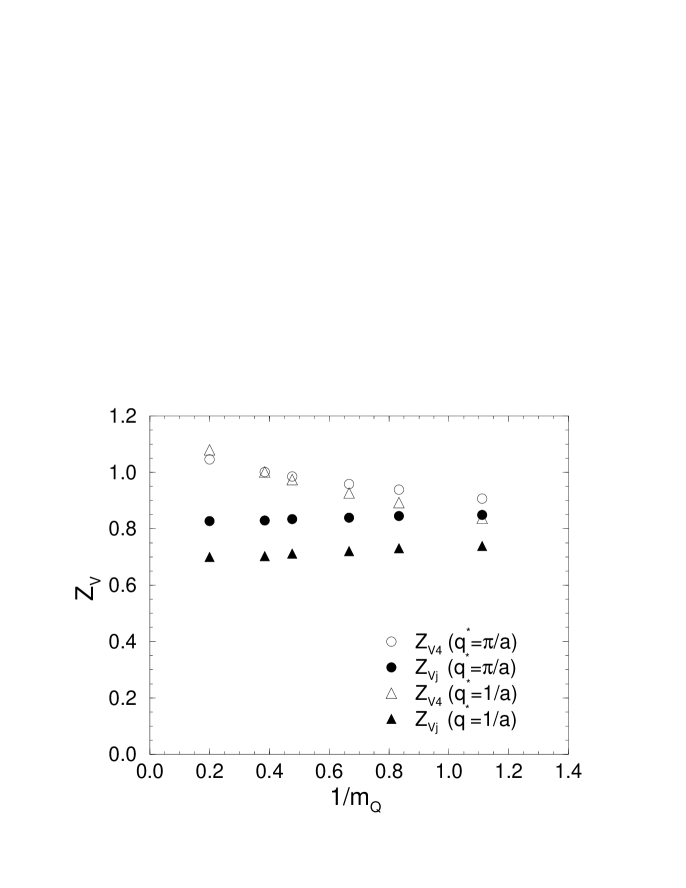
FIG. 1.: Renormalization constant for the vector current with two scales for the coupling constant, $q^{\star}=\pi/a$ and $1/a$. The open and filled symbols represent $Z_{V_{4}}$ and $Z_{V_{j}}$, respectively.

$\kappa=0.1570$

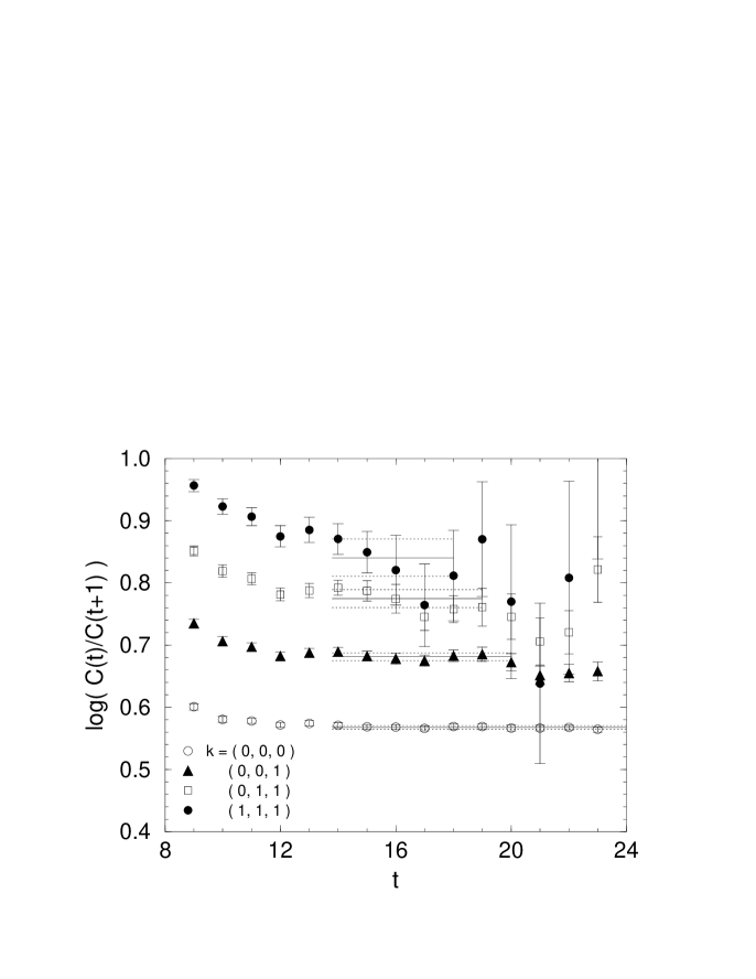
$\kappa=0.1600$

FIG. 2.: Effective mass plot of pion at $\kappa=0.1570$ and $0.1600$. The horizontal solid lines represent the fitted values and the fitting range with the statistical errors (dotted lines).

FIG. 3.: Dispersion relation for pion. The solid lines represent the relation $E_{\pi}^{\,2}(\vec{k})=m_{\pi}^{\,2}+\vec{k}^{2}$ with $m_{\pi}$ the rest mass obtained in the simulation. For $\kappa=0.1585$ and $0.1600$, symbols are slightly shifted in horizontal direction for clarity.

$m_{Q}=2.6$, $\kappa=0.1570$

$m_{Q}=2.6$, $\kappa=0.1600$

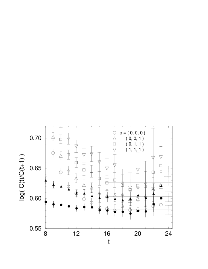
FIG. 4.: Effective mass plot of $B$ meson at $m_{Q}=2.6$ and $\kappa=0.1570$, $0.1600$. Results with the smeared source (filled symbols) are shown for $|\vec{p}|^{2}=0,1$ as well as the results with the local source (open symbols). The horizontal solid lines express the average values over the results of single exponential fit of the local-local and the smeared-local correlation functions. The statistical errors of the fitted values are displayed at the right end of the lines. For all $m_{Q}$, $\kappa$, and momentum, the fit ranges are set to $t=16-24$.

FIG. 5.: Dispersion relation for the $B$ meson at $m_{Q}=2.6$ and $\kappa=0.1570$, $0.1600$. The solid lines represent the relation $E_{\bar{q}Q}(\vec{p})=E_{\bar{q}Q}(0)+\vec{p}^{2}/2m_{B}$, for which $m_{B}$ is determined with the tree level formula $m_{B}=m_{Q}+E_{\bar{q}Q}(0)$. Dashed lines represent the same relation with the renormalized $m_{B}$ at the scale $q^{\star}=1/a$.

$m_{Q}=2.6$, $\kappa=0.1570$, $C_{4}^{(3)}$

$m_{Q}=2.6$, $\kappa=0.1570$, $C_{4}^{(3)}$

$m_{Q}=2.6$, $\kappa=0.1570$,  $\vec{k}\!\cdot\!\vec{C}^{(3)}$

$m_{Q}=2.6$, $\kappa=0.1600$, $C_{4}^{(3)}$

FIG. 6.: Effective mass plot for the three-point functions at $m_{Q}=2.6$ and $\kappa=0.1570$, $0.1600$. The horizontal lines express the values obtained from the two-point correlation functions with the statistical errors indicated at the right end of the lines. Top two figures are for $C_{4}^{(3)}$ and the third is for $\vec{k}\!\cdot\!\vec{C}^{(3)}$ at $\kappa=0.1570$, and bottom figure is for $C_{4}^{(3)}$ at $\kappa=0.1600$.

FIG. 7.: Comparison of $\hat{V}_{4}$ to $(\,E_{B}\hat{U}_{p}+E_{\pi}\hat{U}_{k}\,)$ for $i_{q}=6$ at $\kappa=0.1570$.

FIG. 8.: Chiral extrapolation of the matrix elements for $m_{Q}=2.6$. $V_{4}$ and $\vec{k}\cdot\vec{V}/|\vec{k}|^{2}$ are shown for two momentum configurations $i_{q}=1$, $2$. The solid and the dashed lines represent the linear fit.

FIG. 9.: $\hat{V}_{4}$ at $\kappa=0.1570$. For $\vec{k}=0$ and $|\vec{k}|=1$, the solid and the dashed lines represent the results of linear and quadratic fits, respectively.

FIG. 10.: $\hat{U}_{k}$ at $\kappa=0.1570$. The solid and the dashed lines represent the results of linear and quadratic fits, respectively.

FIG. 11.: Extraction of $\hat{U}_{p}(\vec{p}\!=\!0,\vec{k})$ is shown for $m_{Q}=2.6$ and $1.5$ at $\kappa=0.1570$. The extrapolation is carried out linearly in $\vec{p}^{2}$. For $\vec{k}=0$, $i_{q}=5,13,20$ are used. For $\vec{k}=1$, $\hat{U}_{p}(0,\vec{k})$ is determined using $i_{q}=6,14$, for which $\vec{p}$ and $\vec{k}$ are perpendicular.

FIG. 12.: $\hat{U}_{p}$ multiplied by $m_{B}$ at $\kappa=0.1570$ as a function of $1/m_{B}$. The values of $m_{B}$ are determined with the tree level formula. The solid and the dashed lines represent the linear and the quadratic fits, respectively.

FIG. 13.: One-loop renormalized $\hat{V}_{4}$, $\hat{U}_{k}$, and $\hat{U}_{p}$ as a function of $1/m_{B}$. The solid, the dashed, and the long dashed lines represent the linear fits.

FIG. 14.: Form factors at $m_{Q}=2.6$ and $\kappa=0.1570$, $0.1600$. The solid curves represent the fit to single pole functions.

FIG. 15.: Form factors at $m_{Q}=1.5$ and $\kappa=0.1570$, $0.1600$.

FIG. 16.: $1/f^{0}$ and $1/f^{+}$ as a function of $q^{2}$ at $m_{Q}=2.6$ and $\kappa=0.1570$. The solid and the dotted curves represent the linear and the quadratic fits, respectively. The long dashed line represents the linear fit with the constraint $m_{\mbox{pole}}=m_{B^{*}}$, where $m_{B}^{*}$ is the $B^{*}$ meson mass obtained from the two-point correlation function.

FIG. 17.: $m_{B^{*}}$ obtained from the two-point correlation function of the $B^{*}$ meson and the pole mass from the linear fit of $1/f^{+}$.

FIG. 18.: Renormalized form factors at $m_{Q}=2.6$ and $\kappa=0.1570$. Upper and lower figures are obtained with $g_{V}^{2}(\pi/a)$ and $g_{V}^{2}(1/a)$, respectively. The solid lines represent the results of the linear fit. For $f^{+}(q^{2})$, $\chi^{2}/$dof are $1.9$ and $4.1$ for $q^{*}=\pi/a$ and $1/a$ respectively. $\chi^{2}/$dof for $f^{0}(q^{2})$ are less than $0.5$ in the both cases.

FIG. 19.: Comparison of $f^{0}(q^{2}_{\mbox{max}})$ with $f_{B}/f_{\pi}$ multiplying the factor $\sqrt{m_{B}}$ in the chiral limit. Open and filled symbols are at the tree level and at the one-loop with $g_{V}^{2}(1/a)$, respectively.

FIG. 20.: $f^{0}(q^{2}_{\mbox{max}})$ and $(f_{B}/f_{\pi})m_{B}/(m_{B}+m_{\pi})$ for light quark masses. Two cases of $m_{Q}$, $2.6$ and $1.5$, are displayed at the tree level.

REFERENCES

- [1] C.R. Allton et al. (APE Collaboration), Phys. Lett. B345 (1995) 513; A. Abada et al., Nucl. Phys. B416 (1994) 675.
- [2] D.R. Burford et al. (UKQCD Collaboration), Nucl. Phys. B447 (1995) 425.
- [3] G. Güsken, K. Schilling and G. Siegert, Nucl.Phys. B (Proc. Suppl.) 53 (1996) 485.
- [4] B.A. Thacker and G.P. Lepage, Phys. Rev. D43 (1991) 196; G.P. Lepage et al., Phys. Rev. D46 (1992) 4052.
- [5] For a review, see J. Shigemitsu, Nucl. Phys. B (Proc. Suppl.) 53 (1997) 16.
- [6] For reviews, see T. Onogi, Nucl. Phys. B (Proc. Suppl.) 63 (1998) 59; A. Ali Khan, ibid., 71.
- [7] K.-I. Ishikawa et al., Phys. Rev. D56 (1997) 7028.
- [8] G.P. Lepage and P.B. Mackenzie, Phys. Rev. D48 (1993) 2250.
- [9] K.-I. Ishikawa et al., Nucl. Phys. B (Proc. Suppl.) 63 (1998) 344.
- [10] G.P. Lepage, Nucl. Phys. B (Proc. Suppl.) 26 (1992) 45.
- [11] H. Georgi, Lectures delivered at TASI, Published in Boulder TASI 91, 589 (HUTP-91-A039).
- [12] G. Burdman and J.F. Donoghue, Phys. Lett. B280 (1992) 287; M.B. Wise, Phys. Rev. D45 (1992) R2188.
- [13] N. Kitazawa and T. Kurimoto, Phys. Lett. B323 (1994) 65.
- [14] J.P. Alexander et al. (CLEO Collaboration), Phys. Rev. Lett. 77 (1996) 5000.
- [15] G. Burdman, Z. Ligeti, M. Neubert and Y. Nir, Phys. Rev. D49 (1994) 2331.
- [16] J.N. Simone, Nucl. Phys. B (Proc. Suppl.) 47 (1996) 17.
- [17] J. Shigemitsu, Nucl. Phys. B (Proc. Suppl.) 60A (1998) 134.