THE QCD ABACUS:
A New Formulation for Lattice Gauge Theories 

A quantum Hamiltonian is constructed for SU(3) lattice QCD entirely from color triplet Fermions — the standard quarks and a new Fermionic “constituent” of the gluon we call “rishons”. The quarks are represented by Dirac spinors on each site and the gauge fields by rishon-antirishon bilinears on each link which together with the local gauge transforms are the generators of an SU(6) algebra. The effective Lagrangian for the path integral lives in $R^{4}\times S^{1}$ Euclidean space with a compact “fifth time” of circumference ($\beta$) and non-Abelian charge ($e^{2}$) both of which carry dimensions of length. For large $\beta$, it is conjectured that continuum QCD is reached and that the dimensionless ratio $g^{2}=e^{2}/\beta$ becomes the QCD gauge coupling. The quarks are introduced as Kaplan chiral Fermions at either end of the finite slab in fifth time. This talk will emphasize the gauge and algebraic structure of the rishon or link Fermions and the special properties that may lead to fast discrete dynamics for numerical simulations and new theoretical insight.

1 Introduction

A quarter of a century after its discovery, solving QCD remains one of the major challenges for theoretical particle physics. While Quantum Chromodynamics is generally acknowledged to be a complete theory of all hadronic or nuclear interactions, only special perturbative consequences are well understood. In 1974 a non-perturbative formulation of QCD was given by Wilson $\!{}^{{\bf?}}$ using a lattice regulator which maps the quantum field theory onto a classical statistical mechanics problem in a 4-d Euclidean space. Although a variety of techniques have been developed to solve lattice field theories, at present the most powerful tool is the Monte Carlo sampling of the partition function of the corresponding classical statistical mechanics system. Moreover, the most efficient numerical algorithms for QCD suffer from critical slowing down when the continuum limit is approached and thus overwhelm even the fastest supercomputers. Consequently it is reasonable to look for new formulation of the QCD problem. This talk will present a radically new approach based on recent work by Brower, Chandrasekharan and Wiese $\!{}^{{\bf?}}$. Additional background material for this approach has already been given by Uwe-Jens Wiese in his talk $\!{}^{{\bf?}}$ just preceding this one.

Here we present our alternative non-perturbative approach to QCD in the framework of quantum link models, which leads to a new computational framework we call the QCD Abacus . Such gauge models were first discussed by Horn  $\!{}^{{\bf?}}$, and studied in more detail by Orland and Rohrlich  $\!{}^{{\bf?}}$ and by Chandrasekharan and Wiese $\!{}^{{\bf?}}$. In these models the 4-d classical statistical mechanics problem of standard lattice gauge theory is replaced by a problem of 4-d quantum statistical mechanics. In particular, the classical Euclidean action is replaced by a Hamilton operator. As a consequence, the ordinary c-numbers in the standard formulation of lattice gauge theory for the gauge matrices and their local gauge transformations are replaced by non-commuting operators acting in a Hilbert space. Thus one may say that the geometry of the gauge manifold is replaced by a non-commutative geometry. Nonetheless as discussed in detail in Wiese’s talk, both 4-d non-Abelian quantum link gauge theories and 2-d quantum sigma models are expected to “dimensionally reduce” to an effective continuum field theory exhibiting asymptotically free scaling as the extra compact dimension becomes large (see Fig.1).

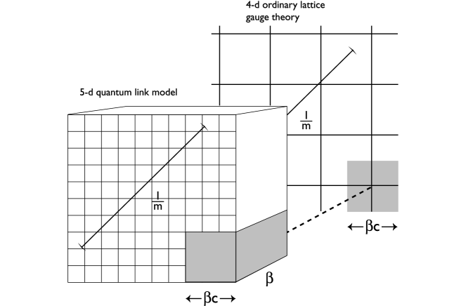
Figure 1: Dimensional reduction in slab geometry: An effective 4-d lattice theory results with lattice spacing $\beta c$ and a gluonic correlation length $1/m$ which is exponential in $\beta$.

These crucial physical motivations will for the most part not be repeated here so the reader is referred to the literature $\!{}^{{\bf?},{\bf?},{\bf?}}$ for them.

In spite of these interesting developments, until the recent paper by Brower, Chandrasekharan and Wiese $\!{}^{{\bf?}}$, no candidate quantum link theory for QCD itself had been proposed due to the difficulty in finding a mechanism to break the U(3) gauge group down to SU(3). All earlier constructions suffered from an extra U(1) gauge symmetry with a strongly coupled “photon” mode which made any serious application to QCD unlikely. Here we describe the algebraic insight that allowed us to construct a candidate quantum link Hamiltonian for QCD. The structure of our proposed QCD quantum link Hamiltonian is elegantly expressed in terms of new Fermionic triplet/anti-triplet fields ($3,\bar{3}$) which in a tight binding mode form “composite” gluonic degrees of freedom. We call these Fermionic constituents of the gauge links, “rishons” or link Fermions $\!{}^{{\bf?}}$. We believe this quantum link formulation of non-perturbative QCD is both correct and compelling for its simplicity. Perhaps it will lead to more powerful methods for attacking long-standing problems in lattice gauge theories by analytical and/or numerical methods.

This talk is organized as follows. In section 2 quantum link models are formulated in terms of rishons — the Fermionic constituents of the gluons. The inclusion of quarks is discussed in section 3 within the framework of Shamir’s variant of Kaplan’s Fermion method. Section 4 contains a discussion of the prospects for deeper theoretical understanding, an analytical approach to the large N limit, for example, and cluster methods for Monte Carlo simulations of quantum link gauge theories.

2 The QCD Abacus

The main goal of this talk is to display the rules for the quantum link Hamiltonian in a form that allows one to appreciate the algebraic structure in a vivid and intuitively appealing form. As illustrated in Fig. 2, the gauge sector of the quantum link QCD Hamiltonian acts on a discrete Fermionic Hilbert space, represented by colored dots for occupied Fermionic states associated with each link. The link occupation level is set to half filling for the sum of left triplet $(3)$ and right anti-triplet $(\bar{3})$ link Fermions. The plaquette term in the Hamilton operator slides the beads in the Abacus along the link in the clockwise or anti-clockwise direction changing the flux by one quantum. Gauge invariance demands that the same color that leaves a site must move into that site from the adjacent link in the plaquette, conserving rishon number for each color at the sites. Another term is introduced into the Hamiltonian to remove the unwanted U(1) gauge invariance which creates and destroys rishon “baryons” at opposite ends of each link, reducing the gauge group from U(3) to SU(3). Once the origin of these rules is explained constructing other quantum link Hamiltonians becomes a natural game of inventing appropriate “cellular automata” rules on the Quantum Abacus.

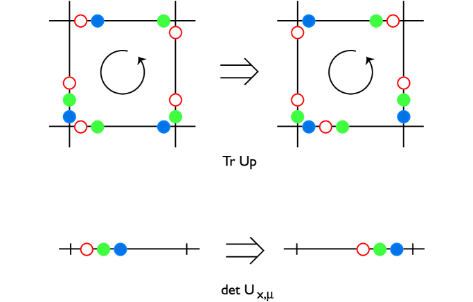
Figure 2: Rishon dynamics: The trace part of the Hamiltonian induces a hopping of rishons of various colors around a plaquette. The determinant part shifts a color-neutral rishon baryon from one end of a link to the other.

At first it may seem hopeless or even paradoxical that one might represent exactly a continuous gauge group (or even a global Lie group) with a finite set of bits per lattice site. However, as discussed in more detail in Wiese‘s talk, a quantum spin is just such an object. For example the electron at rest has only 2 states but still respects exact rotational invariance via quantum superposition. Consequently the trick is to consider the appropriate quantum operators in a discrete Hilbert space. Just as in all quantum systems, the eigenvalues for sets of commuting operators enumerate the states and the operators for Lie group symmetries “rotate” them continuously into linear combinations of these eigenstates.

2.1 U(1) Warm Up Exercise

Before considering the full problem of non-Abelian gauge theory, it is instructive to begin with the simpler compact U(1) Abelian gauge theory. With hindsight many of the basic concepts needed for full QCD can be introduced. Since we want to construct a 4-d gauge Hamiltonian, it is useful (again with the benefit of hindsight) to consider a Kogut-Suskind Hamiltonian  in 4-d as an example,

$$H_{KS}=\frac{e^{2}}{2}\sum_{x,\mu}\hat{E}_{x,\mu}\hat{E}_{x,\mu}+\sum_{x,\mu\neq\nu}\frac{1}{2e^{2}}\hat{U}_{x,\mu}\hat{U}_{x+\mu,\nu}\hat{U}^{\dagger}_{x+\nu,\mu}\hat{U}^{\dagger}_{x,\nu}\;.$$ (1)

The sums extend over lattice sites $x$ and directions $\mu,\nu=1,2,3,4$. Local gauge invariance on each link $(x,x+\mu)$ requires,

$$[\hat{E},\hat{U}]=\hat{U}\;\;\;\;\;\;\;\;[\hat{E},\hat{U}^{\dagger}]=-\hat{U}^{\dagger}\;\;\;\;\;\;\;\;[\hat{U},\hat{U}^{\dagger}]=0\;,$$ (2)

where to simplify the notation the $x,\mu$ subscripts have been dropped .

It is easy to prove (just as with the canonical commutation relations $[\hat{q},\hat{p}]=i$) that the only solutions to this algebra (2) are infinite dimensional “matrices”. For example, in a basis in which all the $\hat{U}$’s are diagonal (the “field basis”), $\hat{E}$ is given by differentiation,

$$\hat{U}\rightarrow e^{\textstyle{i\theta}}\;\;\;\;,\;\;\;\;\hat{E}\rightarrow-i\frac{d}{d\theta}\;,$$ (3)

where $\theta=eA$. On the other hand, if we allow the commutator $[\hat{U},\hat{U}^{\dagger}]$ to be non-zero, finite dimensional representations can be found. This amounts to a new quantum prescription with the group manifold represented as a non-commutative geometry. For example in the smallest representation, the rest of the algebra is easily satisfied by 2 by 2 sigma matrices with

$$\hat{U}\rightarrow{\textstyle{1\over 2}}(\sigma_{1}+i\sigma_{2})\equiv\sigma^{+}\rightarrow\ \left|\begin{array}[]{cc}0&1\\ 0&0\end{array}\right|\;,$$ (4)

$$\hat{U}^{\dagger}\rightarrow{\textstyle{1\over 2}}(\sigma_{1}-i\sigma_{2})\equiv\sigma^{-}\rightarrow\ \left|\begin{array}[]{cc}0&0\\ 1&0\end{array}\right|\;,$$ (5)

and the gauge generator,

$$\hat{E}\rightarrow{\textstyle{1\over 2}}\sigma_{3}\rightarrow{\textstyle{1\over 2}}\ \left|\begin{array}[]{cc}1&0\\ 0&-1\end{array}\right|\;.$$ (6)

In a basis where the E field is diagonal (the “electric basis”), we may view this 2 by 2 representation as simply a truncation of the infinite dimensional representation to a single unit of flux. To show this, let us introduce a set of Fermionic creation/destruction operators,

$$\{c_{l},c^{\dagger}_{l^{\prime}}\}=\delta_{l,l^{\prime}}\;,$$

one for each Fourier mode $l=\pm{\textstyle{1\over 2}},\pm{\textstyle{{3}\over{2}}},\pm{\textstyle{{5}\over{2}}},\cdots,\pm\infty$, and constrain the Hilbert space to

$${\cal N}=\sum_{l}\;c^{\dagger}_{l}c_{l}=1\;.$$

Now the $U(1)$ commutation relations (2) are satisfied by the operators,

$$\hat{U} = \int\frac{d\theta}{2\pi}\phi(\theta)e^{\textstyle{i\theta}}\phi^{\dagger}(\theta)=\sum_{l}c_{l}c^{\dagger}_{l+1}\;,$$ (7)

$$\hat{E} = \int\frac{d\theta}{2\pi}\phi^{\dagger}(\theta)\frac{d}{id\theta}\phi(\theta)=\sum_{l}\;l\;c^{\dagger}_{l}c_{l}\;,$$ (8)

where $\phi(\theta)=\sum_{l}a_{l}e^{\textstyle{il\theta}}$. It is now straight forward to demonstrate that the sole consequence for the algebra of truncating the flux ( i.e. restricting the sum in $\phi(\theta)=\sum_{l}a_{l}e^{\textstyle{il\theta}}$ to $|l|\leq L$ ) is to introduce the non-vanishing commutation relation,

$$[\hat{U},\hat{U}^{\dagger}]=\sum^{L-1}_{l=-L}(c^{\dagger}_{l}c_{l}-c^{\dagger}_{l+1}c_{l+1})\neq 0\;\;.$$

It is important to contrast this truncation procedure in the “electric basis” relative to the more conventional approach of replacing the group manifold by a finite set of angles $\theta_{n}=n\Delta\theta$. In the latter, the continuous symmetry group (i.e. $U(1)$) is, at best, replaced by an approximating subgroup (i.e. $Z_{N}$), whereas by truncating to low dimensional representations in the Fourier space the full symmetry group is left intact!

By taking the lowest non-trivial flux on a link ($l=\pm{\textstyle{1\over 2}}$), we obtain the smallest representation,

$$\hat{U}=ab^{\dagger}\;\;\;\;\hat{U}^{\dagger}=-a^{\dagger}b\;\;\;\;\hat{R}=b^{\dagger}b\;\;\;\;\hat{L}=a^{\dagger}a$$ (9)

where $a\equiv c_{-\frac{1}{2}},b\equiv c_{\frac{1}{2}}$. These satisfy the commutators

$$[\hat{R},\hat{U}]=\hat{U}\;\;\;,\;\;\;[L,\hat{U}]=-\hat{U}\;\;,[\hat{U},\hat{U}^{\dagger}]=\hat{R}-\hat{L}\;\;.$$ (10)

In the 2 dimensional subspace with $a^{\dagger}a+b^{\dagger}b=1$ and $\hat{E}\equiv(\hat{R}-\hat{L})/2$, this reproduces exactly our earlier sigma matrix construction in Eqs. (4-6).

Let us summarize the situation. We can construct a U(1) gauge invariant Hamiltonian acting on a 4-d lattice simply by replacing the link phase factors, $\exp[\pm i\theta]$, by sigma matrices, $\sigma^{\pm}$. The electric field term, being the value of the quadratic Casimir for the lowest dimensional representation, is just an additive constant and can be dropped. The resulting quantum link Hamiltonian for $U(1)$ is

$$\hat{H}=\sum_{x,\mu\neq\nu}\sigma^{+}_{x,\mu}\sigma^{+}_{x+\mu,\nu}\sigma^{-}_{x+\nu,\mu}\sigma^{-}_{x,\nu}$$ (11)

and its partition function is

$$Z=\mbox{Tr}\exp(-\beta\hat{H}).$$ (12)

We note that in this Abelian example, we have made use of two equivalent representation: one in terms of explicit (sigma) matrices and another in terms of link Fermions (or rishons). The strategy in the next section is to explore both of these approaches to generalize this construction to SU(N) Yang-Mills theory.

2.2 U(3) Quantum Link Theory

Let us consider a quantum link Hamiltonian,

$$\hat{H}=\sum_{x,\mu\neq\nu}\mbox{Tr}[\hat{U}_{x,\mu}\hat{U}_{x+\hat{\mu},\nu}\hat{U}_{x+\hat{\nu},\mu}^{\dagger}\hat{U}_{x,\nu}^{\dagger}]\;+\;\cdots$$ (13)

for the non-Abelian field operators $\hat{U}^{ij}_{x,\mu}$. In this Hamiltonian each plaquette is the trace of the matrix product in color indices $i,j=1,\cdots,N$, and a direct product of q number matrix elements. The dots in Eq. 13 represent other operators that will be needed for full QCD, for improved actions, etc.

For SU(3) the local gauge algebra is realized as an $SU_{R}(3)\times SU_{L}(3)$ symmetry for each link operator $\hat{U}$,

$$[\hat{R}_{\alpha},\hat{U}_{ij}]=\hat{U}_{ik}\lambda^{\alpha}_{kj}\;\;\;,\;\;\;[\hat{L}_{\alpha},\hat{U}_{ij}]=-\lambda^{\alpha}_{ik}\hat{U}_{kj}\;\;,$$ (14)

where for notational simplicity we again suppress the link indices $x,\mu$ in the above formula: $\hat{U}\equiv\hat{U}_{x,\mu}$, $\hat{R}\equiv\hat{R}_{x,\mu}$ and $\hat{L}\equiv\hat{L}_{x,\mu}$. Note that each link in fact has 9 operators $\hat{U}_{ij}$ for $i,j=1,2,3$ transforming as a $(3,\bar{3})$ representation . All commutators involving different links are zero. The SU(3) generators obey the Lie algebra,

$$[\hat{R}_{\alpha},\hat{R}_{\beta}]=2if_{\alpha\beta\gamma}\hat{R}_{\gamma}\;\;\;,\;\;\;[\hat{L}_{\alpha},\hat{L}_{\beta}]=2if_{\alpha\beta\gamma}\hat{L}_{\gamma}\;\;\;,\;\;\;[\hat{R}_{\alpha},\hat{L}_{\beta}]=0\;,$$ (15)

where the Gell-Mann matrices  satisfy the algebra,

$$\lambda_{\alpha}\lambda_{\beta}=\delta_{\alpha\beta}+if_{\alpha\beta\gamma}\lambda_{\gamma}+d_{\alpha\beta\gamma}\lambda_{\gamma}\;.$$ (16)

If we introduce infinitesimal generators,

$$\hat{G}^{\alpha}_{x}=\sum_{\mu}(\hat{R}^{\alpha}_{x-\hat{\mu},\mu}+\hat{L}^{\alpha}_{x,\mu})\;,$$ (17)

for local $SU(3)$ gauge transformations, it is trivial to demonstrate that as a consequence of the above Lie algebra the single plaquette Hamiltonian (14) does obey local gauge invariance. Thus we have a general algebraic framework for constructing quantum link Hamiltonians with local gauge invariance. Surely this framework is not unique, but given the reasonable assumption that all non-zero commutators are confined to operators on a single link, it is probably the most natural.

2.3 Minimal Solution

As we will explain in more detail in the next section, there are many solutions to this algebraic problem. Here we attempt to construct the lowest dimensional non-trivial solution, which for U(N) gauge theory will turn out to be built on the smallest irreducible representation of SU(2N). This representation has dimension 2N.

We introduce the ansatz,

$$\hat{U}_{ij}=\delta_{ij}\hat{U}_{0}+i\lambda^{\alpha}_{ij}\hat{U}_{\alpha}=\delta_{ij}\left|\begin{array}[]{cc}0&{\bf 1}\\ 0&0\\ \end{array}\right|+i\lambda^{\alpha}_{ij}\left|\begin{array}[]{cc}0&-i\hat{\Lambda}_{\alpha}\\ 0&0\\ \end{array}\right|$$ (18)

and

$$\hat{R}_{\alpha}=\left|\begin{array}[]{cc}\hat{\Lambda}_{\alpha}&0\\ 0&0\end{array}\right|\;\;\;,\;\;\;\hat{L}_{\alpha}=\left|\begin{array}[]{cc}0&0\\ 0&\hat{\Lambda}_{\alpha}\\ \end{array}\right|\;.$$ (19)

It turns out that the gauge algebra (14) is satisfied, if the q-number link operators $\hat{\Lambda}_{\alpha}$ obey exactly the same Gell-Mann algebra as the c-number generators $\lambda_{\alpha}$,

$$\hat{\Lambda}_{\alpha}\hat{\Lambda}_{\beta}=\delta_{\alpha\beta}+if_{\alpha\beta\gamma}\hat{\Lambda}_{\gamma}+d_{\alpha\beta\gamma}\hat{\Lambda}_{\gamma}\;.$$ (20)

Thus the $\Lambda$’s may also be represented as 3 by 3 matrices for each link. To prove this, substitute the ansatz into Eqs. (14) to get the two relations,

$$\hat{R}_{\alpha}({\bf 1}+\lambda_{\beta}\hat{\Lambda}_{\beta}) = ({\bf 1}+\lambda_{\beta}\hat{\Lambda}_{\beta})\lambda_{\alpha}$$ (21)

$$({\bf 1}+\lambda_{\beta}\hat{\Lambda}_{\beta})L_{\alpha} = \lambda_{\alpha}({\bf 1}+\lambda_{\beta}\hat{\Lambda}_{\beta}).$$ (22)

These are satisfied identically. For example expanding the first relations (21) above yields

$$\hat{\Lambda}_{\alpha}+\lambda_{\alpha}+if_{\alpha\beta\gamma}\lambda_{\beta}\hat{\Lambda}_{\gamma}+d_{\alpha\beta\gamma}\lambda_{\beta}\hat{\Lambda}_{\gamma}=\lambda_{\alpha}+\hat{\Lambda}_{\alpha}+if_{\beta\alpha\gamma}\hat{\Lambda}_{\beta}\lambda_{\gamma}+d_{\beta\alpha\gamma}\hat{\Lambda}_{\beta}\lambda_{\gamma}\;\;.$$ (23)

Using only the condition that $f_{\alpha\beta\gamma}=Tr[[\lambda_{\alpha},\lambda_{\beta}],\lambda_{\gamma}]/6i$ and $d_{\alpha\beta\gamma}=Tr[\{\lambda_{\alpha},\lambda_{\beta}\},\lambda_{\gamma}]/6$ are totally anti-symmetric and symmetric tensors respectively, the identity holds. The second relation (22) is the conjugate of the first. (Clearly the same construction will work for any Lie group.)

In addition to the SU(3) gauge transforms discussed above, there is a pair of left and right U(1) gauge generators,

$$\hat{R}_{0}=\left|\begin{array}[]{cc}{\bf 1}&0\\ 0&0\end{array}\right|\;\;\;,\;\;\;\hat{L}_{0}=\left|\begin{array}[]{cc}0&0\\ 0&{\bf 1}\\ \end{array}\right|\;\;.$$ (24)

The sum, ${\cal N}=R_{0}+L_{0}$, is a trivial symmetry since it commutes with the link operators and the other generators, but the difference, $T=R_{0}-L_{0}$, leads to an additional (unwanted) gauge symmetry,

$$[\hat{T},\hat{U}_{x,\mu}]=2\hat{U}_{x,\mu}\;\;.$$ (25)

The consequence of this extra $U(1)$ generator is that the standard plaquette interaction in our Hamilton operator (13) actually represents a $U(3)$ gauge invariant Yang Mills theory. Indeed because of this unwanted symmetry, all earlier attempts $\!{}^{{\bf?},{\bf?},{\bf?}}$ did not succeed in constructing a Yang-Mills Hamiltonian suitable for QCD with only the SU(3) gauge group.

One way to understand the problem is first to consider the standard single plaquette ($Tr[U_{P}]$) Wilson action and to note that this expression is also invariant with respect to U(3) gauge transformation. Consequently, the restriction to SU(3) for the Wilson theory is in fact introduced “by hand” by defining the path integral with the Haar measure $dU$ restricted to the SU(3) manifold. Therefore, in the quantum case the analogous procedure is to insert a symmetry breaking operator into the trace similarly restricting the phase space. A natural approach (which we will ultimately implement) would be to add to the Hamilton operator a term, $J^{\prime}Det[\hat{U}_{x,\mu}]$, for each link. But in our present minimal construction, the direct product of a link with itself vanishes ( $\hat{U}^{ij}\hat{U}^{kl}=0$), so such a determinant term vanishes identical as an operator! The problem can be traced to the fact that the smallest representation just does not allow one to squeeze more than one unit of flux onto a single link. One (rather inelegant ) way out is to build the SU(3) determinant out of three different operators spreading the flux over three different paths joining the point $x$ to $x+\mu$. Fortunately, the rishon representation will afford a more elegant and minimal solution to constructing the determinant locally on each link.

2.4 The Rishon Representation

We now proceed to this approach to constructing quantum link QCD based on Fermionic triplets (or rishons), which naturally leads to higher dimensional representations of SU(6). The basic algebraic structure of these rishon models is exactly the same as our minimal model given above. In particular all the commutators (and therefore the group properties) are unchanged.

In addition to the gauge commutators (14), let’s enumerate the other commutators. Again the only non-zero commutators for $\hat{U}_{x,\mu}$ and $\hat{U}^{\dagger}_{x,\mu}$ involve the same link $(x,x+\mu$) so we suppress the link index in discussing the algebra. With $\hat{U}=\hat{U}_{0}+i\lambda_{\alpha}\hat{U}_{\alpha}$ and $\hat{U}^{\dagger}=\hat{U}^{\dagger}_{0}-i\lambda_{\alpha}\hat{U}^{\dagger}_{\alpha}$, we have

$$[\hat{U}_{0},\hat{U}^{\dagger}_{0}] = \hat{T}\;,$$ (26)

$$[\hat{U}_{\alpha},\hat{U}^{\dagger}_{\beta}] = \delta_{\alpha\beta}\hat{T}+if_{\alpha\beta\gamma}(\hat{R}_{\gamma}+\hat{L}_{\gamma})+d_{\alpha\beta\gamma}(\hat{R}_{\gamma}-\hat{L}_{\gamma})\,$$ (27)

$$[\hat{U}_{0},\hat{U}^{\dagger}_{\alpha}] = i(\hat{R}_{\alpha}-\hat{L}_{\alpha}).$$ (28)

Also the commutators,

$$[\hat{U}_{\alpha},\hat{U}_{\beta}]=0\;\;,\;\;[\hat{U}^{\dagger}_{\alpha},\hat{U}^{\dagger}_{\beta}]=0\;,$$ (29)

are zero for all $\alpha,\beta=0,\cdots N^{2}-1$. In addition in the minimal construction above, we also have the nil potency property that $\hat{U}_{x,\mu}$ and $\hat{U}^{\dagger}_{x,\mu}$ just as in the U(1) gauge theory act like a creation-destruction operators: $\hat{U}_{x,\mu}^{2}=\hat{U}^{\dagger 2}_{x,\mu}=0$. Not being part of the Lie algebra, we will see that this special nil potency condition is a peculiarity of the lowest dimensional representation.

The rishon construction begins with the following ansatz. Consider $2N$ Fermionic operators $a_{i}$ and $b_{i}$ for $i=1,\cdots,N$, with anti-commutators,

$$\{a_{i},a^{\dagger}_{j}\}=\delta_{ij}\;\;\;,\;\;\;\{b_{i},b^{\dagger}_{j}\}=\delta_{ij}\;,$$ (30)

on each link and all other anti-commutators zero between different links and between a’s and b’s on the same link. The local gauge rotations are

$$\hat{L}_{\alpha}=\sum_{i}a^{\dagger}_{i}\lambda^{\alpha}_{ij}a_{j}\;\;\;,\;\;\;\hat{R}_{\alpha}=\sum_{i}b^{\dagger}_{i}\lambda^{\alpha}_{ij}b_{j}\;,$$ (31)

on each link with $\alpha=0,1\cdots N^{2}-1$. Just as in traditional current algebras, these bilinears obviously satisfies the correct $SU_{R}(N)\times SU_{L}(N)$ gauge algebra. The gauge fields are then represented by

$$\hat{U}_{ij}=\sum_{\alpha=0}^{N^{2}-1}\lambda^{\alpha}_{ji}\;a_{n}\lambda^{\alpha}_{nm}b^{\dagger}_{m},$$ (32)

or

$$\hat{U}_{ij}=a_{i}b^{\dagger}_{j}\;,$$ (33)

since the $N^{2}$ $\lambda$’s form a complete hermitian basis. Again it is straight forward to see that the complete set of bilinears made from $2N$ Fermi fields must give the Lie Algebra relations for $SU(2N)$. There is a very appealing interpretation. The bosonic gauge field is a Fermion-anti-Fermion bound state. Like the tight binding Hamiltonians of solid state physics, these “rishons” constituents never move relative to each other, so there are no new internal degrees of freedom.

The rishon bilinears act on a $2^{2N}$ dimensional Fock space at each link which can be enumerated by occupation numbers $0,1$ for each Fermionic mode: $a^{\dagger}_{i},b^{\dagger}_{i}$. Moreover the entire algebra commutes with the link number operator,

$${\cal N}=\hat{R}_{0}+\hat{L}_{0}=\sum_{i}a^{\dagger}_{i}a_{i}+\sum_{i}b^{\dagger}_{i}b_{i}\;,$$ (34)

so that the $2^{2N}$ dimensional matrices are reducible into a set of $2N+1$ irreducible representations. The enumeration of the representations go as follows. The link number $\hat{R}_{0}+\hat{L}_{0}=K$ extends over $K=0,1,\cdots 2N$, but there is a $Z_{2}$ particle-hole symmetry that relates $K$ to $2N-K$ so really the models are distinguished only for $K=0,1,\cdots N$. The case K = 0 is trivial. Consequently, there are only N distinct representations. For U(1) there is a unique model which is exactly the one discussed above in Section 2.1. For general N, the case K = 1 corresponds to a $2N$ dimensional representation, since the Fock space is restricted to a single Fermion with one of the $a_{i}$’s or one of the $b_{i}$’s occupied. This is exactly the minimal U(N) construction presented above. The models with $K>1$ are new. For SU(2), K = 2 is a 6 dimensional representation of SU(4) (anti-symmetric two index tensors). The square of a link field now has one nonzero component given by

$$det[\hat{U}_{x,\mu}]=\frac{1}{2!}\;\epsilon_{ij}\;\epsilon_{i^{\prime}j^{\prime}}\hat{U}^{i,i^{\prime}}_{x,\mu}\hat{U}^{j,j^{\prime}}_{x,\mu}=2!\;a^{1\dagger}_{x,\mu}a^{2\dagger}_{x,\mu}b^{1}_{x,\mu}b^{2}_{x,\mu}.$$ (35)

Consequently a term which breaks U(2) down to SU(2) can be introduce locally on a single link in the 6 dimensional representation. For SU(3) there are two new models — for $K=2$, a 15 dimensional representations with $\hat{U}^{2}$ non-zero but $\hat{U}^{3}=0$ and for $K=2$, a 20 dimensional representations with $\hat{U}^{3}$ non-zero. Just as in SU(2), the 20 dimensional representation allows a U(1) breaking term to be introduced on a single link,

$$det[\hat{U}_{x,\mu}]=\frac{1}{3!}\;\epsilon_{ijk}\;\epsilon_{i^{\prime}j^{\prime}k^{\prime}}\;\hat{U}^{i,i^{\prime}}_{x,\mu}\hat{U}^{j,j^{\prime}}_{x,\mu}\hat{U}^{k,k^{\prime}}_{x,\mu}=3!\;a^{1\dagger}_{x,\mu}a^{2\dagger}_{x,\mu}a^{3\dagger}_{x,\mu}b^{1}_{x,\mu}b^{2}_{x,\mu}b^{3}_{x,\mu}\;.$$ (36)

The intermediate case for SU(3) with K = 2 will allow U(1) breaking to be introduced on a single plaquette coupling a di-rishon with a rishon. Clearly there is a tradeoff between the size of the representation and the ability to represent operators locally on the lattice.

In summary, we pick our candidate Hamilton operator for SU(N) Yang-Mills theory to be

$$\hat{H} = J\sum_{x,\mu\neq\nu}\sum_{i,j,k,m}a^{i}_{x,\mu}b^{j\dagger}_{x,\mu}a^{j}_{x+\hat{\mu},\nu}b^{k\dagger}_{x+\hat{\mu},\nu}b^{k}_{x+\hat{\nu},\mu}a^{m\dagger}_{x+\hat{\nu},\mu}b^{m}_{x,\nu}a^{i\dagger}_{x,\nu}$$

$$+ J^{\prime}\sum_{x,\mu}\ N!\;[a^{1}_{x,\mu}b^{1\dagger}_{x,\mu}a^{2}_{x,\mu}b^{2\dagger}_{x,\mu}...a^{N}_{x,\mu}b^{N\dagger}_{x,\mu}+b^{1}_{x,\mu}a^{1\dagger}_{x,\mu}b^{2}_{x,\mu}a^{2\dagger}_{x,\mu}...b^{N}_{x,\mu}a^{N\dagger}_{x,\mu}]$$

The plaquette part of the Hamilton operator shifts single rishons from one end of a link to the other and simultaneously changes their color. The determinant part, on the other hand, shifts an entire “rishon-baryon” — a color neutral combination of $N$ rishons — along the link. Each link is restricted to a half filled state of N rishons by fixing,

$$a^{i\dagger}_{x,\mu}a^{i}_{x,\mu}+b^{i\dagger}_{x,\mu}b^{i}_{x,\mu}=N\;,$$

so that the link algebra carries a $2N!/(N!N!)$ dimensional irreducible representation. This rather simple rishon dynamics may facilitate new analytic approaches to QCD, and may also be useful in numerical simulations of quantum link models as discussed in Section 3.

2.5 Comments on SU(2) Gauge Actions

SU(2) was the first example of SU(N) Yang Mills theory formulated as a quantum link model $\!{}^{{\bf?}}$. For SU(2) there is a special simplicity, which allowed the link operators $\hat{U}_{\mu}$ to be represented by $\gamma_{\mu}$ matrices in an SO(5) algebra, but this special feature tended to obscured further generalizations. With our general rishon method for SU(N), it is natural to ask if this special SO(5) construction for the SU(2) model represents a distinct alternative. In fact this is not the case. Following the rishon construction, one can develop the SO(5) algebra for SU(2) as a limiting case.

Returning to our minimal construction presented in Sec. 2.3, the algebraic distinction between SU(2) and SU(N) is due to the d-symbol. To remove the extra U(1) gauge invariance for SU(2), one makes use of another form of the link operator, $\hat{V}_{ij}=(\sigma_{2}\hat{U}^{\dagger}\sigma_{2})_{ji}$ that also obeys the same gauge algebra for SU(2), where $\hat{U}$ is given by the expression in Eq. 18. This is possible for SU(2) because there is an extra G parity symmetry: $\sigma_{\alpha}\rightarrow\sigma_{2}\sigma_{\alpha}\sigma_{2}=-\sigma^{*}_{\alpha}=-\sigma_{\alpha}^{T}$ that preserves the algebra. (Note invariance of $\sigma_{\alpha}\sigma_{\beta}=\delta_{\alpha\beta}+i\epsilon_{\alpha\beta\gamma}\sigma_{\gamma}$ under $\sigma_{\alpha}\rightarrow-(\sigma_{\alpha})^{T}$.) In other words for SU(2), the $(2)$ and $(\bar{2})$ representations, which are related by the raising and lowering symbols ( $\epsilon_{ij}=\epsilon^{ij}=i(\sigma_{2})_{ij}$), are unitarily equivalent.

However if we attempt the same construction for SU(3) by introducing,

$$\hat{V}=\left|\begin{array}[]{cc}0&0\\ {\bf 1}&0\\ \end{array}\right|+i\lambda_{\alpha}\left|\begin{array}[]{cc}0&0\\ i\hat{\Lambda}_{\alpha}&0\\ \end{array}\right|\;\;,$$ (38)

the new fields fail to obey the gauge algebra (14),

$$-({\bf 1}-\lambda_{\beta}\hat{\Lambda}_{\beta})\hat{R}_{\alpha} \neq ({\bf 1}-\lambda_{\beta}\hat{\Lambda}_{\beta})\lambda_{\alpha}\;\;,$$ (39)

$$\hat{L}_{\alpha}({\bf 1}-\lambda_{\beta}\hat{\Lambda}_{\beta}) \neq -\lambda_{\alpha}({\bf 1}-\lambda_{\beta}\hat{\Lambda}_{\beta})\;\;,$$ (40)

due to the opposite sign for the d-symbols on the right and left hand sides. Consequently only for SU(2), do we have the special construction,

$$\hat{H}_{SU(2)}=\frac{J}{4}\sum_{x;\mu>\nu}\mbox{Tr}[{\cal U}_{x,\mu}{\cal U}_{x+\hat{\mu},\nu}{\cal U}_{x+\hat{\nu},\mu}^{\dagger}{\cal U}_{x,\nu}^{\dagger}]\;,$$ (41)

where the new link operators are a sum of two terms, ${\cal U}_{x,\mu}=\hat{U}_{x,\mu}+\hat{V}_{x,\mu}$. Note also that $U={\cal U}(1+T)/2$ and $V={\cal U}(1-T)/2$. This Hamiltonian is “by accident” both hermitian and gauge invariant under SU(2) but not U(2).

However another construction is also possible for SU(3), beginning with the minimal 6 dimensional representation in Eq. 18. This is based on the observation that any link $\hat{U}(x,y)$ connecting $x$ to $y$, transforms as a $(3,\bar{3})$ representation of $U_{R}(3)\times U_{L}(3)$. Thus not only can we form U(3) gauge singlets by contractions with $\delta_{ij}$’s to make “mesons” at the sites but we can also form SU(3) singlets by contractions with $\epsilon_{ijk}$’s to make “baryons” at the sites. For example we can add a term,

$$\hat{H}_{1}=J_{1}\sum_{<x,y>}\epsilon_{ijk}\;\hat{U}^{(1)}_{i,i^{\prime}}(x,y)\hat{U}^{(2)}_{j,j^{\prime}}(x,y)\hat{U}^{(3)}_{k,k^{\prime}}(x,y)\;\epsilon_{i^{\prime}j^{\prime}k^{\prime}}$$ (42)

where the $U^{\prime}s$ are 3 independent paths between x and y.

In the special case of U(2), one may use two paths connecting $x$ and $y$ on a single plaquette. With appropriate weights and paths, this procedure can lead you back to the earlier SO(5) suggestions for an SU(2) Hamiltonians (41). For example, take

$$\hat{H}_{1}=J_{1}\sum_{<x,y>}\epsilon_{ij}\;\hat{U}^{(1)}_{i,i^{\prime}}(x,y)\hat{U}^{(2)}_{j,j^{\prime}}(x,y)\;\epsilon_{i^{\prime}j^{\prime}}\;.$$ (43)

Making use of the raising and lowering symbol $\epsilon_{ij}=(i\sigma_{2})_{ij}$, this expression can be re-written as

$$\hat{H}_{1}=J_{1}\sum_{<x,y>}\hat{U}^{(1)}_{ij}(x,y)\hat{V}^{(2)}_{j,i}(y,x)$$ (44)

Identifying $\hat{U}^{(1)}$ and $\hat{V}^{(2)}$ with products of links on the edges of the plaquette, we get the individual terms in Eq. 41 that break U(1) gauge symmetry. The former choice (41) is just one possible Hamiltonian, where the epsilon symbol is inserted or not into all the corners of the plaquette with equal weight.

3 Quark Fields and Full QCD

To represent full QCD, one must add quarks to the quantum link model. This is more or less straightforward, although some subtleties arise related to the dimensional reduction of Fermions $\!{}^{{\bf?}}$.

Again the guiding principle is to replace the classical action of the standard formulation by a Hamilton operator which describes the evolution of the system in a fifth Euclidean direction. For the quarks this implies replacing the Grassmann variables $\psi_{x},\bar{\psi}_{x}$ by $\Psi_{x},\Psi^{\dagger}_{x}\gamma_{5}$, where $\Psi^{\dagger}_{x}$ and $\Psi_{x}$ are quark creation and annihilation operators with canonical anti-commutation relations

$$\{\Psi^{ia\alpha}_{x},\Psi^{jb\beta\dagger}_{y}\}=\delta_{xy}\delta_{ij}\delta_{ab}\delta_{\alpha\beta},\ \{\Psi^{ia\alpha}_{x},\Psi^{jb\beta}_{y}\}=\{\Psi^{ia\alpha\dagger}_{x},\Psi^{jb\beta\dagger}_{y}\}=0,$$ (45)

where $(i,j)$, $(a,b)$ and $(\alpha,\beta)$ are color, flavor and Dirac indices, respectively.

The full QCD quantum link Hamiltonian is now given by

$$\hat{H} = J\sum_{x,\mu\neq\nu}\mbox{Tr}[\hat{U}_{x,\mu}\hat{U}_{x+\hat{\mu},\nu}\hat{U}^{\dagger}_{x+\hat{\mu},\nu}\hat{U}^{\dagger}_{x,\nu}]+J^{\prime}\sum_{x,\mu}\ [\mbox{det}\hat{U}_{x,\mu}+\mbox{det}\hat{U}^{\dagger}_{x,\mu}]$$ (46)

$$+ {\textstyle{1\over 2}}\sum_{x,\mu}\ [\Psi^{\dagger}_{x}\gamma_{5}\gamma_{\mu}\hat{U}_{x,\mu}\Psi_{x+\hat{\mu}}-\Psi^{\dagger}_{x+\hat{\mu}}\gamma_{5}\gamma_{\mu}\hat{U}^{\dagger}_{x,\mu}\Psi_{x}]+\sum_{x}\Psi^{\dagger}_{x}\gamma_{5}{\cal M}\Psi_{x}$$

$$+ \frac{r}{2}\sum_{x,\mu}\ [2\Psi^{\dagger}_{x}\gamma_{5}\Psi_{x}-\Psi^{\dagger}_{x}\gamma_{5}\hat{U}_{x,\mu}\Psi_{x+\hat{\mu}}-\Psi^{\dagger}_{x+\hat{\mu}}\gamma_{5}\hat{U}^{\dagger}_{x,\mu}\Psi_{x}].$$

The generators of $SU(N)$ gauge transformations must include quark bilinears,

$$\hat{G}^{\alpha}_{x}=\sum_{\mu}(\hat{R}^{\alpha}_{x-\hat{\mu},\mu}+\hat{L}^{\alpha}_{x,\mu})+\Psi^{\dagger}_{x}\lambda^{\alpha}\Psi_{x}\;,$$ (47)

but it is still trivial to show that $\hat{H}$ commutes with all $\hat{G}^{\alpha}_{x}$.

To ensure the proper dimensional reduction of the quarks, their boundary conditions in the fifth direction must be chosen appropriately. The standard antiperiodic boundary conditions, which are dictated by thermodynamics in the Euclidean time direction, would lead to Matsubara modes, $p_{5}=2\pi(n_{5}+\frac{1}{2})/\beta$. However for our 5-th time, this would lead to a mass of $O(\beta)$ for the dimensionally reduced quark. On the other hand, the confinement physics of the induced 4-d gluon theory takes place at a correlation length which grows exponentially with $\beta$. Therefore, quarks with antiperiodic boundary conditions in the fifth direction would remain at the cut-off freezing out the quarks and returning the dimensionally reduced theory to a quarkless pure Yang-Mills theory. One possible solution is obvious. Simply choose periodic boundary conditions for the quarks in the fifth direction. This gives rise to a Matsubara mode, $p_{5}=0$, that survives dimensional reduction. Since the extent of the fifth direction has nothing to do with the inverse temperature (which is the extent of the Euclidean time direction), one could indeed choose the boundary condition in this way.

There is another perhaps more attractive possibility. The above scenario with periodic boundary conditions for the quarks still suffers from the same fine tuning problem as the original Wilson Fermion method. The bare mass matrix $\cal M$ would have to be adjusted very carefully in order to reach the chiral limit. In practice this is a serious problem for numerical simulations. This problem has been solved very elegantly in Shamir’s variant  $\!{}^{{\bf?}}$ of Kaplan’s Fermion proposal  $\!{}^{{\bf?}}$. Kaplan studied the physics of a 5-d system of Fermions, which is always vector-like, coupled to a 4-d domain wall that manifests itself as a topological defect. The key observation is that under these conditions a zero mode of the 5-d Dirac operator appears as a bound state localized on the domain wall. From the point of view of the 4-d domain wall, the zero mode represents a massless chiral Fermion. The original idea was to construct lattice actions for chiral gauge theories in this way.

Subsequently, Shamir pointed out that the same mechanism can also be used to solve the lattice fine tuning problem of the bare Fermion mass in vector-like theories like QCD. He also suggested a variant of Kaplan’s method that has several technical advantages, and that turns out to fit very naturally with the construction of quantum link QCD. In quantum link models, we already have a fifth direction for reasons unrelated to the chiral symmetry of Fermions. We will now follow Shamir’s proposal, and use the fifth direction to solve the fine tuning problem that we would have with periodic boundary conditions for the quarks. The essential technical simplification compared to Kaplan’s original proposal is that one now works with a 5-d slab of finite size $\beta$ with open boundary conditions for the Fermions at the two sides. This geometry limits one to vector-like theories, because now there are two zero modes — one at each boundary — which correspond to one left and one right-handed Fermion in four dimensions. This approach fits naturally with our construction of quantum link QCD. In particular, the evolution of the system in the fifth direction is still governed by the Hamilton operator of Eq. 46. The only difference relative to Wilson’s Fermion method is that now $r<0$.

The partition function of the theory with open boundary conditions for the quarks and with periodic boundary conditions for the gluons is given by

$$Z=\mbox{Tr}\langle 0|\exp(-\beta H)|0\rangle.$$ (48)

Here the trace extends only over the gluonic Hilbert space of the quantum link model, thus implementing periodic boundary conditions for the gluons. The boundary conditions for the Fermions are realized by taking the expectation value of $\exp(-\beta H)$ in the Fock state $|0\rangle$, which is annihilated by all right-handed $\Psi_{Rx}$ and by all left-handed $\Psi^{\dagger}_{Lx}$  $\!{}^{{\bf?}}$. As a result, there are no left-handed quarks at the boundary at $x_{5}=0$, and there are no right-handed quarks at the boundary at $x_{5}=\beta$. Of course, unlike periodic or antiperiodic boundary conditions, open boundary conditions for the Fermions break translation invariance in the fifth direction. Through the interaction between quarks and gluons, this breaking also affects the gluonic sector. We don’t expect this to be problematic, because we are only interested in the 4-d physics after dimensional reduction. The only crucial feature is that both quarks and gluons have zero modes that survive dimensional reduction.

There is one technical detail. We have argued before that the gluonic correlation length is not truly infinite as long as $\beta$ is finite, but — due to confinement — it is exponentially large. The same is true for the quarks, but for a different reason. In fact, already free quarks pick up an exponentially small mass due to tunneling between the two boundaries, which mixes left-handed and right-handed states, and thus breaks chiral symmetry explicitly.

The important observation is that the bare mass parameter $M$ (considering a single flavor for the moment) is not the physical quark mass. The physical mass of the quark goes exponentially fast to zero in $\beta$ in the continuum limit without fine tuning. At the same time, the doubler modes remain at the cut-off. Let us first consider the doubler Fermions, which are characterized by $n=1,2,3,4$ for the corners of the Brillouin zone. It can be shown $\!{}^{{\bf?}}$ that the doubler masses diverge, if we choose

$$M+2nr<0.$$ (49)

In fact this precise inequality applies for non-interacting quarks with zero gauge fields. But close to the continuum limit, we expect nearly the same inequalities. Thus there is a region with $r<-M/2$, for a sufficiently strong Wilson-term with an unconventional sign, where the doubler Fermions are removed from the physical spectrum. On the other hand, the mass of the physical Fermion (the $n=0$ state) is

$$\mu=|E(\vec{0})|=2M\exp(-M\beta),$$ (50)

which is exponentially small in $\beta$, again up to small corrections when we turn on the gauge fields in weak coupling. These results indicate how one may avoid the fine-tuning problem of the Fermion. The confinement physics of quantum link QCD in the chiral limit takes place at a length scale,

$$\xi\propto\exp(\frac{24\pi^{2}\beta}{(11N-2N_{f})Ne^{2}}),$$ (51)

which is determined by the 1-loop coefficient of the $\beta$-function of QCD with $N_{f}$ massless quarks and by the 5-d gauge coupling $e$. As long as one chooses

$$M>\frac{24\pi^{2}}{(11N-2N_{f})Ne^{2}},$$ (52)

the fictitious induced mass for the chiral quark is exponentially smaller than the QCD scale $\Lambda_{QCD}$ and there is a window in which the chiral limit is reached automatically as one approaches the continuum limit taking $\beta$ large. For a given value of $r$ one is limited by $M<-2r$ (note that $r<0$). On the other hand, one can always choose $J$ (and thus $e^{2}$) such that the above inequality is satisfied. The corresponding geometry is shown in Fig. 3.

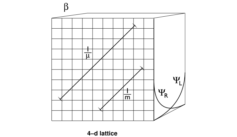
Figure 3: Dimensional reduction in slab geometry: The gluonic correlation length $1/m$ is exponential in $\beta$. Left and right-handed quarks live on the two sides of the slab. The overlap of their wave functions $\Psi_{R}$ and $\Psi_{L}$ induces a mass $\mu$. The corresponding correlation length $1/\mu$ is exponentially larger than $1/m$.

Of course, we also want to be able to work at non-zero quark masses. Following Shamir, we do this by modifying the boundary conditions for the quarks in the fifth direction. Instead of using $\psi_{L}(\vec{x},x_{4},0)=\psi_{R}(\vec{x},x_{4},\beta)=0$ we now demand

$$\psi_{L}(\vec{x},x_{4},0)=-\frac{m}{2M}\psi_{L}(\vec{x},x_{4},\beta),\ \psi_{R}(\vec{x},x_{4},\beta)=-\frac{m}{2M}\psi_{R}(\vec{x},x_{4},0),$$ (53)

where $m$ is a mass parameter. This reduces to the previous boundary condition for $m=0$, while it corresponds to antiperiodic boundary conditions for $m=2M$, and to periodic boundary conditions for $m=-2M$. Solving the above equations with the new boundary condition indeed yields physical quarks of mass $m$ in the continuum limit $\beta\rightarrow\infty$ as long as $m\ll M$. It has been shown in Ref. References that in the interacting theory $m$ is only multiplicatively renormalized. On the level of the partition function,

$$Z=\mbox{Tr}[\exp(-\beta H){\cal O}(m)]\;,$$ (54)

the new boundary condition manifests itself by a mass-dependent operator,

$${\cal O}(m)=\prod_{x}(\Psi_{Rx}\Psi^{\dagger}_{Rx}+\Psi^{\dagger}_{Rx}\frac{m}{2M}\Psi_{Rx})(\Psi^{\dagger}_{Lx}\Psi_{Lx}+\Psi_{Lx}\frac{m}{2M}\Psi^{\dagger}_{Lx}),$$ (55)

which was constructed by Furman and Shamir $\!{}^{{\bf?}}$. Note that in Eq. 54 the trace is both over the gluonic and over the Fermionic Hilbert space. In the chiral limit $m=0$, the operator ${\cal O}(m)$ reduces to a projection operator $|0\rangle\langle 0|$ on the Fock state introduced before. For $m=2M$, i.e. for antiperiodic boundary conditions, the operator ${\cal O}(m)$ becomes the unit operator, and the partition function reduces to the well-known expression from thermodynamics. For $m=-2M$, i.e. for periodic boundary conditions, the operator ${\cal O}(m)$ becomes an alternating sign $(-1)^{F}$ where $F$ is the total fermion number and the trace becomes a super trace.

4 Concluding Remarks

In this brief talk, I have attempted to outline the algebraic steps required to convert a standard lattice gauge theory into a quantum link theory for the QCD Abacus. This has resulted in a demonstration that we can in fact construct a 4-d quantum link Hamiltonian for quarks and gluons which obey all the constraints of local gauge invariance and discrete symmetries for QCD. There has not been time in this talk for many other important theoretical issues such as why we believe this is a legitimate alternative formulation of lattice QCD or time to report on the substantial progress being made to convert our new scheme to a viable theoretical and computational tool. In a sense for quantum link QCD, we now have to repeat the last 20 years of work that has been done in the Wilson formulation.

Although it has not been emphasized, it should be plausible that our general approach to converting a classical action into a corresponding Hamiltonian operating on a discrete space in one extra dimension can be applied to a wide range of quantum field theories. In fact we have coined the term “D-theory” for the general class of quantum spin and quantum link theories that are obtained by such a discrete “re-quantization” of path integral expressions $\!{}^{{\bf?}}$. In some ways the procedure in D-theory is analogous to the construction of M-theory whereby the string co-ordinates for the world sheet embedded in 10 dimensions are replace by matrices living in 10+1 dimensions. When the extra dimension is compactified, the ratio ($e^{2}/\beta$) of the 11-d coupling ($e^{2}$) and the compact circumference ($\beta$) becomes the coupling ($g^{2}$) in the 10-d dimensionally reduce theory: $e^{2}/\beta\rightarrow g^{2}$. The general procedure in D-theory is to study the symmetry properties of the target field theory and to replace the co-ordinates (i.e. fields) with a non-commuting algebra that expresses all the basic symmetries. Once the representations for the fundamental quantum spins (matter fields) and quantum links (gauge fields) have been chosen, a large variety of Hamiltonians can be defined. If there is a zero gap in the d+1 dimensional D-theory before compactification of the extra dimension, then we believe that dimensional reduction to and universality with the target field theory is generally assured.

The use of anti-commuting fields to build finite dimensional representations of symmetry groups (i.e. rishons in our terminology) is of course a widely used device. Indeed the rishon formulation resembles the Schwinger boson and constraint Fermion constructions of quantum spin systems  $\!{}^{{\bf?}}$. Just as it has for spins models this trick may provide new theoretical insight leading perhaps to new analytic approaches to QCD, for example, in the large $N$ limit. In particular we note that the Hamilton operator (46) of quantum link QCD with a $U(N)$ gauge group (i.e. dropping the determinant term) can also be expressed in terms of color singlet glueball, meson and constituent quark operators. These objects consist of two rishons, two quarks and a quark-rishon pair, respectively. To see this, just contract the color triplet indices in Eq. 46, defining color singlet bilinears for the new fields,

$$\Phi_{x,+\mu,+\nu}=c^{i\dagger}_{x,\mu}c^{i}_{x,\nu}\;\;,\;\;M^{a\alpha b\beta}_{x}=\Psi^{ia\alpha\dagger}_{x}\Psi^{ib\beta}_{x}\;\;,\;\;Q^{a\alpha}_{x,+\mu}=c^{i\dagger}_{x,\mu}\Psi^{ia\alpha}_{x}\;,$$ (56)

representing glueball, meson and constituent quark mesons respectively. In this formula, we have defined $c^{i}_{x,\mu}=a_{x,\mu}$ and $c^{i}_{x,-\mu}=b^{i}_{x,\mu}$ for $\mu=1,2,3,4$. The $8+4N_{f}$ triplet fermion operators obviously combine as bilinears to give the generators for an $SU(16+8N_{f})$ algebra. In principle this theory can be bosonized in terms of these degrees of freedom. If large $N$ techniques can be applied successfully, major progress in the non-perturbative solution of QCD and other interesting field theories is to be expected. In any case, it is intriguing that $U(N)$ quantum link QCD has two representations — one exclusively in terms of colored quark and rishon Fermions, the other in terms of color-singlet bosons. Returning to SU(N) only adds rishon baryons to the set of color singlet fields.

Although it has not been emphasized in this talk, one can argue $\!{}^{{\bf?},{\bf?},{\bf?}}$ that there is a reasonable scenario for this theory to undergo dimensional reduction so that the continuum limit is reached for large values of the 5-th time extensions $\beta$ and that the resulting theory is universally equivalent to Wilson’s formulation of QCD. Let us remind ourselves of the analogous situation for the conventional Wilson formulation. Here the “demonstration” that lattice QCD gives the correct continuum theory involved re-deriving renormalized perturbation theory from the lattice and showing numerically that the confined phase extends to zero (bare) coupling with asymptotically free scaling. In spite of numerous technical difficulties, there is a general consensus that these tests have been met for the Wilson approach. While we have not yet accomplished a similar degree of certainty for the quantum link formulation, we believe it can be accomplished. For Quantum link QCD, perturbation theory is more difficult, but we have begun to consider a coherent state formalism which in principle will allow one to define “spin waves” (i.e. gluons) around a weak coupling vacuum. These spin waves should interact in weak coupling like ordinary QCD perturbation theory.

One approach is to begin with the equations of motion for the quantum link Hamiltonian,

$$\frac{d}{dt}\hat{U}_{x,\mu} = i[\hat{H},\hat{U}_{x,\mu}]\;\;,\;\;\frac{d}{dt}\hat{T}_{x,\mu}=i[\hat{H},\hat{T}_{x,\mu}]\;$$

$$\frac{d}{dt}\hat{R}^{\alpha}_{x,\mu} = i[\hat{H},\hat{R}^{\alpha}_{x,\mu}]\;\;,\;\;\frac{d}{dt}\hat{L}^{\alpha}_{x,\mu}=i[\hat{H},\hat{L}^{\alpha}_{x,\mu}]\;.$$ (57)

and argue that in the appropriate classical limit, they lead as expected to the 5-d Yang-Mills equation for the mean fluctuations ,

$$A_{\mu}(x)=\frac{1}{2i}<\hat{U}(x+\mu,x)-\hat{U}^{\dagger}(x+\mu,x)>\;,$$ (58)

about the vacuum $<\hat{U}>=1$ in the “5-th time” $A_{5}=0$ gauge. In addition, we are investigating the phase structure of 5-d QCD to establish the existence of a gapless Coulomb phase $\!{}^{{\bf?},{\bf?}}$. The mechanism we postulate for dimensional reduction of gauge theories is that compactifying the 5-th time leads to a gap and confinement. As argued by Wiese and Chandrasekharan $\!{}^{{\bf?}}$, this follows closely an analogy with dimensional reduction of the quantum spin Hamiltonians for 2-d non-linear sigma models, where there is also a target asymptotically free theory and the gap is guaranteed by the Mermin-Wagner-Coleman theorem $\!{}^{{\bf?}}$. Interestingly, in a non-Abelian gauge theory, the analog of the Mermin-Wagner-Coleman theorem is confinement itself. The direct demonstration of this mechanism for quantum link gauge theories (since no one has succeeded to date in defining the confining vacuum) will probably come from numerical simulations, where in the slab geometry one identifies asymptotic freedom emerging as $\beta$ is increased. This will require efficient Monte Carlo algorithms.

There is one last issue of tremendous promise and importance that must be mentioned. In simulations, the potential advantage of the quantum link approach is the application of cluster algorithms as typified by the classic Swendsen-Wang algorithm $\!{}^{{\bf?}}$ that has revolutionized simulations for the Ising model and other classical spin systems $\!{}^{{\bf?},{\bf?}}$. In a cluster algorithm entire regions of spatially correlated variables are “flipped” together. This can have spectacular results near the continuum limit (or more generally a second order phase transition) in reducing critical slowing down. In the standard Wilson formulation of gauge theories, no such cluster algorithm has ever been found for models with a continuous gauge group. For the U(1) quantum link model, we have succeed in formulating and implementing the first such cluster algorithm.

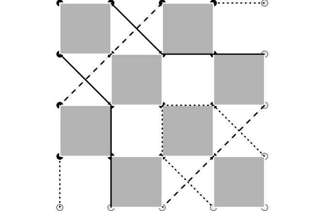
Figure 4: The figure shows a typical graph in 1d with $L=4$, and $N=2$. Every white square represents a two spin interaction. The graph shown here splits the lattice into three clusters, represented by a solid line, broken line and a dotted line.

The cluster methods for the gauge model are being developed by a close analogy with 2-d cluster algorithms for quantum spin systems. For quantum spin systems, successful cluster algorithms have already been invented $\!{}^{{\bf?},{\bf?}}$ and very impressive result obtain in simulations $\!{}^{{\bf?},{\bf?}}$. For example efficient cluster algorithms for a quantum XY models (analogous to a U(1) gauge theory) have been studied and we know how to construct $\!{}^{{\bf?}}$ improved estimators for quantum Green’s functions such as $<\sigma^{+}_{x}\sigma^{-}_{x}>$. By use of an explicit basis for the transfer matrix and the Trotter formula, one has a quantum generalization of the Fortuin-Kasteleyn map onto a random cluster model. The clusters for the quantum XY model are single closed curves in the d+1 space (see Fig 4). We can prove detailed balance and basis independence for the quantum matrix elements $\!{}^{{\bf?}}$. Also one can formulate these algorithms exactly on the continuous “time” interval $[0,\beta]$ making no error due to the usual Trotter formula approximation.

Remarkably an analogous procedure has been carried out for the U(1) gauge theory $\!{}^{{\bf?}}$. The most interesting topological difference with quantum spin system is that now the clusters are closed surfaces (instead of closed lines) representing world sheets for string states propagating in the extra time direction. As in all efficient cluster algorithms with improved estimators, the structure of the clusters should signify a new set of collective co-ordinates which play an important role in the dynamics. For quantum link theory these collective co-ordinates evidently are indicative of an underlying stringy vacuum.

Finally we should remark that in the general formulation of a particular D-theory, we expect that there are many alternative lattice Hamiltonians that are universally equivalent after dimensional reduction, but have different microscopic details. This flexibility at the microscopic level is (ultimately) a strength. Just as solvable 2-d spin systems, beginning with the classic work on the Ising model, have led to new theoretical insight (i.e. critical scaling) and new algorithms (i.e. percolation cluster methods), a particular formulation of quantum link models may lead to more efficient algorithms or more tractable analytic methods. The implication is that detailed choices among possible universally equivalent options should go hand in hand with the development of analytical and numerical methods. There are many options that we are exploring that go beyond the examples I have had time to present. Nonetheless we feel there is a rather clear unified methodology in constructing a D-theory and ample reason for optimism that they can contribute new insight into the nature of asymptotically free field theories.

References

References

- [1] K. Wilson, Phys. Rev. D10 (1974) 2445.
- [2] R. C. Brower, S. Chandrasekharan and U-J Wiese, “QCD as a Quantum Link Model”, hep-th/9704106.
- [3] U-J Wiese Quantum Spins and Quantum Links: From Antiferromagnets to QCD in this volume (1997).
- [4] D. Horn, Phys. Lett. 100B (1981) 149.
- [5] P. Orland and D. Rohrlich, Nucl. Phys. B338 (1990) 647.
- [6] S. Chandrasekharan and U.-J. Wiese, Nucl. Phys. B492 (1997) 455.
- [7] R. Brower, R. Giles, and G. Maturana. “Link Fermions in Euclidean Lattice Gauge Theory” Phys. Rev. (1984) D29:704.
- [8] Y. Shamir, Nucl. Phys. B406 (1993) 90.
- [9] D. B. Kaplan, Phys. Lett. B288 (1992) 342.
- [10] V. Furman and Y. Shamir, Nucl. Phys. 439 (1995) 54.
- [11] R. Brower, S. Chandrasekharan and U.-J. Wiese, in preparation.
- [12] A. Auerbach, “Interacting Electrons and Quantum Magnetism”, Springer, New-York (1994).
- [13] M. Creutz, Phys. Rev. Lett. 43 (1979) 553.
- [14] R. C. Brower, S. Chandrasekharan, D. Chen and U.-J Wiese, in preparation.
- [15] N. D. Mermin and H. Wagner, Phys. Rev. Lett. 17 (1966) 1133; S. Coleman, Commun. Math. Phys. 331 (1973) 259.
- [16] R. Swendsen and S.-J. Wang, Phys. Rev. Lett. 58 (1987) 86.
- [17] U. Wolff, Phys. Rev. Lett. 62 (1989) 361; Nucl. Phys. B334 (1990) 581.
- [18] R. C. Brower and P. Tamayo, Phys. Rev. Lett. 62 (1989) 1087
- [19] H. G. Evertz, G. Lana and M. Marcu, Phys. Rev. Lett. 70 (1993) 875.
- [20] U.-J. Wiese and H.-P. Ying, Z. Phys. B93 (1994) 147.
- [21] B. B. Beard and U.-J. Wiese, Phys. Rev. Lett. 77 (1996) 5130.
- [22] B. B. Beard, A. Ferrando, M. Greven and U.-J. Wiese, in preparation.
- [23] R. Brower, S. Chandrasekharan and U.-J. Wiese, in preparation.
- [24] M. Basler, B. B. Beard, R. Brower, S. Chandrasekharan, A. Tsapalis and U.-J. Wiese, in preparation.