Abstract

Gauge-invariant non-local scalar and field strength operators have been argued to have significance, e.g., as a way to determine the behaviour of the screened static potential at large distances, as order parameters for confinement, as input parameters in models of confinement, and as gauge-invariant definitions of light constituent masses in bound state systems. We measure such “correlators” in the 3d pure SU(2) and SU(2)+Higgs models on the lattice. We extract the corresponding mass parameters and discuss their scaling and physical interpretation. We find that the finite part of the $\overline{\mbox{\rm MS}}$ scheme mass measured from the field strength correlator is large, more than half the glueball mass. We also determine the non-perturbative contribution to the Debye mass in the 4d finite $T$ SU(2) gauge theory with a method due to Arnold and Yaffe, finding $\delta m_{D}\approx 1.06(4)g^{2}T$.

1 Introduction

The strength and range of forces described by gauge theories are characterized by the potential of a static charge. Non-Abelian pure gauge theories in three and four dimensions are known to be confining in the sense that the potential in the fundamental representation rises linearly with distance. If matter fields are added the static potential is modified: the linear rise persists only up to a critical distance at which enough energy is stored in the flux tube to pair create matter. The matter particles will then be separated and form bound states with the sources, so that the rise of the static potential saturates at the energy of the two bound state systems. If one considers static sources in the adjoint representation instead, the potential again rises linearly, but is supposed to saturate even in the pure gauge theory due to the creation of a pair of gluons.

In this work, we investigate non-perturbatively operators related to the energy of the bound state systems created after the breaking of the flux tube in the pure SU(2) and SU(2)+Higgs models. The non-local gauge-invariant operators measured consist of sources of a given charge coupled via a Wilson line in the same representation:

$$G_{\phi}(x,y) \equiv {\frac{1}{2}}\left\langle{\rm Tr\,}\phi^{\dagger}(x)U^{\rm fund}(x,y)\phi(y)\right\rangle,$$ (1)

$$G_{F,ijkl}(x,y) \equiv \left\langle F^{a}_{ij}(x)U^{\rm adj}_{ab}(x,y)F^{b}_{kl}(y)\right\rangle.$$ (2)

The fundamental Wilson line here is $U^{\rm fund}(x,y)={\cal P}\exp({ig\int_{x}^{y}\!dx_{i}A_{i}^{a}T^{a}})$ and the adjoint Wilson line is $U^{\rm adj}_{ab}(x,y)=2{\rm Tr\,}T^{a}U^{\rm fund}(x,y)T^{b}[U^{\rm fund}(x,y)]^{\dagger}$, where $T^{a}=\sigma^{a}/2$ and $\sigma^{a}$ are the Pauli matrices.

More specifically, the mass signal $M$ extracted from these operators has a number of applications. First, related to the discussion above, $M$ is naively expected to determine the asymptotic value to which the static potential saturates, $V(\infty)=2M$ (see below). The most prominent way of calculating the static potential is to extract it from the expectation value of large Wilson loops measured in lattice Monte Carlo simulations. In four dimensions (4d) this has been done for the fundamental representation ([1] and references therein) as well as for the adjoint representation ([2] and references therein). Analogous calculations in three dimensions (3d) may be found in [3, 4]. However, no hard evidence for the saturation of the potential could be obtained in these calculations. One possible explanation is that the string in a lattice simulation does not break because of a potentially bad projection of the Wilson loop onto the hadronized final state. Furthermore, Wilson loop calculations are very expensive in computer time. However, assuming the validity of the above picture of flux tube breaking, one may combine knowledge of the static potential at small distances with its asymptotic value obtained from measuring $M$, to arrive at a rough estimate of the critical distance where the potential flattens off, i.e., the “screening length”.

Second, the asymptotic behaviour of $G_{\phi}(x,y)$ constitutes an order parameter for the phase of the theory: in a Coulomb phase, $G_{\phi}(0,y)\sim\exp(-m|y|)/|y|^{(d-1)/2}$, whereas in a confinement or Higgs phase, the behaviour should be purely exponential [5].

Third, the parameters related to the operator $G_{F,ijkl}(x,y)$ contain important non-perturbative information about the QCD ground state [6] and may hence act as input parameters in models of confinement, such as the stochastic vacuum model [7, 8] (for recent references see, e.g., [9–11]). This is of relevance also in 3d, since 3d theories can be regarded as laboratories for studying the qualitative features of confinement in QCD [12, 13]. The advantage of the 3d theories is that they are superrenormalizable and, consequently, exhibit very good scaling behaviour so that one can extrapolate results of lattice simulations to the continuum limit with an accuracy at the percent level [14, 15]. One especially useful feature of the SU(2)+Higgs model is that the presence of the Higgs doublet allows a smooth interpolation between the non-perturbative confinement and the perturbative Higgs regimes [16, 13]. The physical significance of the 3d theories stems from the fact that they constitute the high temperature effective theories of usual 4d theories in the framework of dimensional reduction [17, 18].

Fourth, in analogy with the heavy – light quark system [19], the mass parameters extracted from $G_{\phi}(x,y)$ and $G_{F,ijkl}(x,y)$ can be viewed as determining the masses of the light dynamical constituents in meson-like bound states. This aspect can be of relevance, e.g., for the constituent models proposed to apply in the (symmetric) confinement phase of the 3d SU(2)+Higgs model [8, 20]. In this context, the Wilson line operators have also been conjectured [20] to explain the value of the propagator mass obtained from a simulation in a fixed Landau gauge [21].

Finally, related to the determination of the light constituent mass of a bound state, the operator $G_{F,ijkl}(x,y)$ in the pure 3d SU(N) theory can be used to measure the leading non-perturbative contribution to the finite temperature Debye mass in 4d SU(N) QCD [22]. The connection to 4d physics is again via dimensional reduction.

The purpose of this paper is to measure the operators in eqs. (1), (2) in 3d (in 4d, these operators have been studied on the lattice in [2, 23]). We improve upon the measurements of $G_{F,ijkl}(x,y)$ performed for pure 3d SU(2) in [4], and extend the measurements to the SU(2)+Higgs case including now also the operator $G_{\phi}(x,y)$ (some properties of $G_{\phi}(x,y)$ have been previously studied in [24]). The discretization of the operators in eqs. (1), (2) is explained in Sec. 2. Some perturbative calculations are performed in Sec. 3. The technical details of the simulations are given in Sec. 4 and the numerical results are presented in Sec. 5. In Sec. 6 we discuss the physical implications of our results for the various topics sketched above, and Sec. 7 comprises the conclusions.

2 The lattice operators and the connection to the static potential

The continuum Lagrangian of the 3d SU(2)+Higgs model is

$${\cal L}={\frac{1}{4}}F^{a}_{ij}F^{a}_{ij}+(D_{i}\varphi)^{\dagger}D_{i}\varphi+m_{3}^{2}\varphi^{\dagger}\varphi+\lambda_{3}(\varphi^{\dagger}\varphi)^{2}.$$ (3)

On the lattice, one introduces $\phi=(\tilde{\varphi}\;\varphi)$, where $\tilde{\varphi}=i\sigma_{2}\varphi^{*}$ and $\sigma_{2}$ is the Pauli matrix. After a rescaling of $\phi$, the lattice action is ($P_{ij}$ is the plaquette)

$$S[\phi,U] = \beta_{G}\sum_{x}\sum_{i<j}[1-{\frac{1}{2}}{\rm Tr\,}P_{ij}]-\beta_{H}\sum_{x}\sum_{i}{\frac{1}{2}}{\rm Tr\,}\phi^{\dagger}(x)U_{i}(x)\phi(x+\hat{i})$$ (4)

$$+ \sum_{x}(1-2\beta_{R}){\frac{1}{2}}{\rm Tr\,}\phi^{\dagger}(x)\phi(x)+\beta_{R}\sum_{x}\bigl{[}{\frac{1}{2}}{\rm Tr\,}\phi^{\dagger}(x)\phi(x)\bigr{]}^{2}.$$

In order to make contact with the calculations in [15] we fix the ratio of the continuum scalar and gauge couplings to be

$$x\equiv\frac{\lambda_{3}}{g_{3}^{2}}=\frac{\beta_{R}\,\beta_{G}}{\beta_{H}^{2}}=0.0239.$$ (5)

At this parameter value the Higgs model exhibits a strong first-order phase transition upon variation of $\beta_{H}$, or $y\equiv m_{3}^{2}/g_{3}^{4}$ in continuum notation. We pick the same two points in parameter space as in [15], namely $y=0.089$ and $y=-0.020$, representing the confinement and Higgs phase, respectively. Once $\beta_{G}$ is chosen, the appropriate values of $\beta_{H}$ and $\beta_{R}$ are determined by the “lines of constant physics” which govern the approach of the 3d theory to the continuum limit [25]. Results for the pure gauge theory may be obtained by considering only gluonic operators and simulating at $\beta_{H}=0$.

Consider then the gauge-invariant two-point function in eq. (1). The path $\Gamma$ between $x$ and $y$ could be for instance a rectangular one as shown in Fig. 1(a). However, it has been demonstrated by simulations in the 4d SU(2)+Higgs model that the coefficient $M$ of the exponential decay of $G_{\phi}(x,y)$ is independent of $R$ [23]. Hence, we restrict attention to $R=0$ in the following. Choosing $T$ to be in the 3-direction the simplest choice representing eq. (1) is then

$$G_{\phi}(T)=\left\langle{\frac{1}{2}}{\rm Tr\,}\left[\phi^{{\dagger}}(x)S(x,T)\phi(y)\right]\right\rangle,$$ (6)

with

$$S(x,T)=\prod_{n=0}^{N-1}U_{3}(x+n\hat{3}),\qquad y=x+N\cdot\hat{3},$$ (7)

and $T=Na$. In practice, we average this operator over the whole lattice in order to improve statistics. One can also choose fundamental charge operators other than the $\phi$’s at the ends of the Wilson line (see Sec. 4). The expectation (to be tested below) is that for large $T$, $G_{\phi}(T)$ should decay as $\exp{(-M\,T)}$ both in the Higgs and in the screened confinement phase [5].

Figure 1: The operators measured on the lattice: (a) The correlator $G_{\phi}(x,y)$ with a fundamental Wilson line (in practice we have $R=0$, and the correlator is denoted by $G_{\phi}(T)$). (b) The correlator $G_{F}(T)$ with an adjoint Wilson line.

The connection to the static potential and to screening is provided by employing the standard picture of string breaking through matter pair production. Assuming that the expectation value of the Wilson loop has a perimeter law behaviour for a large closed loop $C$, $W(R,T)\propto\exp(-M|C|)=\exp[-2M(R+T)]$, the static potential, defined as $\widetilde{V}(R)=-\lim_{T\to\infty}[\ln W(R,T)]/T$ or

$$V(R)=-\lim_{T\to\infty}\ln\left[\frac{W(R,T)}{W(R,T-1)}\right],$$ (8)

obeys

$$V(R\rightarrow\infty)=2M.$$ (9)

Here $M$ is assumed to be the same mass parameter as measured from eq. (6), when an optimal choice is made for the operator at the ends of the Wilson line. The physical interpretation of eq. (9) is that at infinite separation of the static sources, the static potential consists just of the energy of the hadronized system with each static source binding a dynamical charge.

Consider then the case of a static source in the adjoint representation. The Wilson line in the time direction now has to be taken in the adjoint representation, and the gluon field binding to it is described by a spatial plaquette. Hence we consider the gauge-invariant correlator shown in Fig. 1(b),

$$G_{F,ijkl}(T)=\left\langle 4{\rm Tr\,}(P_{ij}(x)T^{a})\Gamma^{ab}(T){\rm Tr\,}(P^{{\dagger}}_{kl}(y)T^{b})\right\rangle,$$ (10)

where

$$\Gamma^{ab}(T)=2{\rm Tr\,}\left(T^{a}S(x,T)T^{b}S^{{\dagger}}(x,T)\right),$$ (11)

and $S$ and $y$ are as in eq. (7). This may be rewritten as

$$G_{F,ijkl}(T) = \left\langle 2{\rm Tr\,}\left[P_{ij}(x)SP^{{\dagger}}_{kl}(y)S^{{\dagger}}\right]-\frac{2}{N}{\rm Tr\,}P_{ij}(x){\rm Tr\,}P_{kl}(y)\right\rangle$$ (12)

$$= \left\langle{\rm Tr\,}\left[P_{ij}(x)S\left(P^{{\dagger}}_{kl}(y)-P_{kl}(y)\right)S^{{\dagger}}\right]\right\rangle,$$

where the last equality holds for SU(2) only. In our simulation, we use $G_{F}$ in this last form, with the components $ij=kl=12$; we omit the spatial indices of $G_{F}(T)\equiv G_{F,1212}(T)$ in the following. The plaquettes are replaced by the sum over all four spatial plaquettes of the same orientation sharing the end points of the Wilson lines, i.e. $P(x)\equiv P_{12}(x)+P_{12}(x-\hat{1})+P_{12}(x-\hat{2})+P_{12}(x-\hat{1}-\hat{2})$. To improve on the statistics, we again average over the whole lattice. Adjoint charge operators other than $P_{ij}$ can be considered as well (see Sec. 4).

The relation to the static potential may be taken over from the fundamental case. It is known that the static potential in this case also shows a linear rise due to flux tube formation between the static charges. As the flux tube now is in the adjoint representation it couples to the gauge fields and thus is expected to break even in the case of pure gauge theory. The corresponding final state consists of the static adjoint source binding a dynamical gluon, a system that has been termed “glue-lump” in the literature [2, 4].

3 Perturbation theory

Although the purpose of this paper is a non-perturbative measurement of the correlators in eqs. (1), (2), let us in this section study these quantities perturbatively. The main motivation is to see how the mass parameters measured depend on the lattice spacing $a$. We will also make some other computations in the Higgs and confinement phases.

3.1 Scaling with the lattice spacing

The mass parameters measured from eqs. (1), (2) turn out to contain a divergent part $\propto g_{3}^{2}\ln(a)$. There is no counterterm in which to absorb this divergence so that, in fact, there is no meaningful continuum limit. Nevertheless, measurements with a finite lattice spacing can be useful for a number of applications, as we will see. Due to the fact that the gauge coupling is dimensionful in 3d, the divergent part can be determined with a 1-loop computation. Moreover, it can be seen that the only such contribution comes from the Wilson line, depicted in Fig. 2. Following [22], let us thus consider this object.

Figure 2: The Wilson line self-energy in the fundamental (a) and adjoint (b) representation.

Letting the Wilson line be an infinitely long straight line in the $z$-direction, expanding the path-ordered exponential to second order in the fields and taking the derivative with respect to $z$, one finds for the coefficient $M$ in the exponential fall-off,

$$M = g_{3}^{2}\lim_{z\to\infty}\frac{d}{dz}\left[\int_{0}^{z}\!dy\int_{0}^{y}\!dx\langle A^{a}_{z}(x,{\bf 0})A^{b}_{z}(y,{\bf 0})\rangle\right](T^{a}T^{b})_{\alpha\beta}$$ (13)

$$= g_{3}^{2}\int_{0}^{\infty}dx\langle A^{a}_{z}(x,{\bf 0})A^{b}_{z}(0,{\bf 0})\rangle(T^{a}T^{b})_{\alpha\beta}$$

$$= g_{3}^{2}C_{2}{\frac{1}{2}}\int\frac{d^{2}p_{\perp}}{(2\pi)^{2}}\frac{1}{p_{\perp}^{2}+m_{W}^{2}}.$$

Here $\alpha=\beta$ are isospin indices not summed over, $C_{2}=N$ for the adjoint representation, and $C_{2}=(N^{2}-1)/(2N)$ for the fundamental representation. The gauge field propagator was taken in a general gauge in the Higgs phase of the SU(2)+Higgs model with the mass $m_{W}$. The result in eq. (13) applies also on the lattice when the integration range is restricted to $(-\pi/a,\pi/a)$ and the momentum in the propagator is replaced with $p_{\perp}^{2}\to\tilde{p}_{\perp}^{2}=\sum_{i=1}^{2}\tilde{p}_{i}^{2}$, where $p_{i}=({2}/{a})\sin({ap_{i}}/{2})$. The intergal in eq. (13) can be computed and one gets

$$\int_{-\pi/a}^{\pi/a}\!\!\frac{d^{2}p}{(2\pi)^{2}}\frac{1}{\tilde{p}^{2}+m^{2}} = \frac{1}{4\pi}\ln\left(\frac{32}{m^{2}a^{2}}\right)+{\cal O}(a)\quad\quad({\rm lattice}),$$ (14)

$$\int\!\!\frac{d^{2-2\epsilon}p}{(2\pi)^{2-2\epsilon}}\frac{1}{p^{2}+m^{2}} = \frac{\mu^{-2\epsilon}}{4\pi}\left(\frac{1}{\epsilon}+\ln\frac{\overline{\mu}^{2}}{m^{2}}\right)\quad\quad\quad(\mbox{\rm$\overline{\mbox{\rm MS}}$ in continuum}),$$ (15)

which provides a relation between the two schemes. Eqs. (13), (14) tell how the mass parameters measured on the lattice depend on the lattice spacing.

In the following, we will want to consider quantities which do have a continuum limit. From eqs. (13), (14), it can be seen that this is obtained by subtracting from $M$ a divergent part:

$${M^{\prime}}\equiv{M}-{g_{3}^{2}}\frac{C_{2}}{8\pi}\ln\left(\frac{32}{g_{3}^{4}a^{2}}\right)={M}-{g_{3}^{2}}\frac{C_{2}}{4\pi}\ln\left(\frac{2\sqrt{2}\beta_{G}}{N}\right),$$ (16)

where $\beta_{G}=2N/(g_{3}^{2}a)$ for SU(N). Here the mass scale needed to define the logarithm in eq. (14) was chosen to be $g_{3}^{2}$. The quantity $M^{\prime}$ is a continuum quantity in the sense that in the $\overline{\mbox{\rm MS}}$ scheme with the scale $\overline{\mu}=g_{3}^{2}$, the exponential fall-off is determined by

$$M_{\overline{\mbox{\rm\tiny MS}}}=M^{\prime}+g_{3}^{2}\frac{C_{2}}{8\pi}\frac{1}{\epsilon}.$$ (17)

Figure 3: The graphs contributing to the correlator $G_{\phi}(T)$ in the Higgs phase at 1-loop order. A dashed line is a Higgs field, a wiggly line a gauge field, a double line a ghost field and the cross denotes a counterterm. A filled circle is the shifted field $\hat{\varphi}$, whereas an open circle is the quantum field $\varphi^{\prime}$.

3.2 Higgs phase

Let us then consider the correlator $G_{\phi}(T)$ in the Higgs phase of the SU(2)+Higgs model in some more detail. The Higgs field is thus written as $\varphi=\hat{\varphi}+\varphi^{\prime}$, $\hat{\varphi}\neq 0$. At leading order, one gets just the constant $\hat{\varphi}^{\dagger}\hat{\varphi}$. The graphs contributing at the next order are shown in Fig. 3. The other graphs are straightforward, so let us consider the Wilson line contribution, (3.c). For arbitrary $T$, we get

$$\left.G_{\phi}(T)\right|_{\rm(3.c)} = {\frac{3}{2}}\biggl{[}-f(\xi^{1/2}m_{W},T)+f(\xi^{1/2}m_{W},0)+f(m_{W},T)-f(m_{W},0)$$ (18)

$$-2\int_{-\pi/a}^{\pi/a}\!\!\frac{d^{3}p}{(2\pi)^{3}}\frac{m_{W}^{2}}{\tilde{p}^{2}+m_{W}^{2}}\frac{\sin^{2}(\frac{p_{z}T}{2})}{\tilde{p}_{z}^{2}}\biggr{]}.$$

Here $\xi$ is the gauge fixing parameter of an $R_{\xi}$ gauge and

$$f(m,|z|)=\int_{-\pi/a}^{\pi/a}\!\!\frac{d^{3}p}{(2\pi)^{3}}\frac{e^{ip\cdot z}}{\tilde{p}^{2}+m^{2}},$$ (19)

with the limiting values ($\Sigma=3.175911535625$)

$$f(m,0)=\frac{\Sigma}{4\pi a}-\frac{m}{4\pi}+O(am^{2}),\quad f(m,z)\stackrel{{\scriptstyle|z|\gg 1/m}}{{\longrightarrow}}\frac{e^{-m|z|}}{4\pi|z|}.$$ (20)

The gauge parameter dependent parts in eq. (18) cancel those form the other graphs, so that the result is explicitly gauge independent. In the limit $T\to\infty$, eq. (18) is dominated by a linear term, $\left.G_{\phi}(T)\right|_{\rm(3.c)}\to\hat{\varphi}^{\dagger}\hat{\varphi}(-MT)$, where $M$ is from eqs. (13), (14) with $C_{2}=3/4$.

Including also the other graphs, the complete 1-loop answer for large $T$ is

$$G_{\phi}(T) = \hat{\varphi}^{\dagger}\hat{\varphi}\left[1-T\frac{3g_{3}^{2}}{16\pi}\ln\frac{4\sqrt{2}}{m_{W}a}\right]$$ (21)

$$+ \frac{\Sigma}{4\pi a}\left(1+{\frac{3}{4}}\frac{g_{3}^{2}}{\lambda_{3}}\right)-f(m_{H},0)-{\frac{3}{4}}\frac{g_{3}^{2}}{\lambda_{3}}f(m_{W},0)$$

$$+ \frac{1}{8\pi}m_{H}+\frac{3}{4\pi}m_{W}+\frac{e^{-m_{H}T}}{8\pi T}+\frac{3}{4\pi}\frac{e^{-m_{W}T}}{m_{W}T^{2}}+O(a)+O\left(\frac{1}{mT}\right),$$

where $m_{W},m_{H}$ are the perturbative $W$ and Higgs masses, respectively. The $1/a$-term on the 2nd row cancels the divergences from $f(m_{H},0)$, $f(m_{W},0)$, so that the sum is finite. At $T=0$, on the other hand, the result is the first two rows plus a divergent term $\Sigma/(2\pi a)$.

In the Higgs phase for $G_{\phi}(T)$, one can thus see explicitly how a pure exponential behaviour arises, after the exponentiation into $\hat{\varphi}^{\dagger}\hat{\varphi}\exp(-MT)$ of the first row in eq. (21) (analytic arguments for the exponentiation can be obtained with the cumulant expansion, see, e.g., [26]). This is in contrast to the typical perturbative terms on the 3rd row containing pre-exponential corrections. It will be seen that the pure exponential is indeed what is observed on the lattice.

For the vector correlator in the Higgs phase, the corresponding computation is much more tedious. At the continuum limit one may write

$$P_{ij}(x)\approx e^{ia^{2}g_{3}T^{a}F^{a}_{ij}(x)}$$ (22)

in eq. (10), and the leading term in the $\overline{\mbox{\rm MS}}$ scheme is

$$G_{F}(T)\propto\langle F^{a}_{12}(0)F^{a}_{12}(T)\rangle\approx(N^{2}-1)\frac{m_{W}}{2\pi T^{2}}e^{-m_{W}T}.$$ (23)

Taking into accout the next order, one gets a contribution $\exp(-M^{\rm adj}T)$ from the Wilson line multiplying eq. (23), where, according to eqs. (13), (14),

$$M^{\rm adj}=\frac{g_{3}^{2}}{2\pi}\ln\frac{4\sqrt{2}}{am_{W}}.$$ (24)

However, there are many other contributions as well (in pure 4d SU(N) in the continuum, the graphs have recently been computed in [10]). We will not evaluate these graphs explicitly. It will be seen that on the lattice the behaviour of $G_{F}(T)$ is again favoured to be purely exponential rather than with a prefactor as in eq. (23), and that the exponent is $\sim m_{W}+M^{\rm adj}$.

3.3 Confinement phase

Consider then the confinement phase of the SU(2)+Higgs model, or the pure SU(2) theory. From eqs. (13), (14) it is immediately seen that a perturbative computation of the correlators is not possible: the tree-level mass parameter $m_{W}$ vanishes so that the IR-regime makes $M$ divergent. One can only extract the coefficient of the logarithm which determines how the mass $M$ scales when the lattice spacing $a$ is varied.

There is, however, the following meaningful computation one can make [22]. (These considerations are in complete analogy with those for the heavy – light quark system in 4d, see [19].) To be specific, consider the 3d SU(2)+adjoint Higgs theory,

$$L={\frac{1}{4}}F^{a}_{ij}F^{a}_{ij}+{\frac{1}{2}}(D_{i}A_{0})^{a}(D_{i}A_{0})^{a}+{\frac{1}{2}}(m_{D}^{\mbox{\scriptsize LO}})^{2}A_{0}^{a}A_{0}^{a}+{\frac{1}{4}}\lambda_{A}(A_{0}^{a}A_{0}^{a})^{2},$$ (25)

where the mass parameter $m_{D}^{\mbox{\scriptsize LO}}$ is large. Suppose one wants to compute the mass $M_{HL}$ of the “heavy–light” bound state $h_{i}=\epsilon_{ijk}A_{0}^{a}F^{a}_{jk}$. A perturbative computation meets immediately with IR-problems [22, 27]. In addition, lattice simulations in the full theory are difficult since the requirement $aM_{HL}\ll 1$ is very stringent, due to the heavy constituent mass $m_{D}^{\mbox{\scriptsize LO}}$ (see, however, [28]). On the other hand, perturbation theory does work for integrating out $A_{0}$, since there are no IR-problems due to the large mass. Therefore, one can integrate $A_{0}$ out analytically, replacing $\langle h_{i}(0)h_{i}(T)\rangle$ by precisely the correlator $G_{F}(T)$ in eq. (2) in the pure 3d SU(2) theory, times an overall factor. The only subtlety is that the heavy mass $M_{H}\sim m_{D}^{\mbox{\scriptsize LO}}$ appearing in the overall factor gets modified in the integration procedure. As a result, the mass signal $M$ measured from $G_{F}(T)$ represents the difference

$$M=M_{HL}-M_{H},$$ (26)

where $M_{H}$ is determined by the computation in [22] to be (for $\lambda_{A}\ll g_{3}^{2}$)

$$M_{H}=m_{D}^{\mbox{\scriptsize LO}}+\frac{Ng_{3}^{2}}{8\pi}\left[\ln\frac{(am_{D}^{\mbox{\scriptsize LO}})^{2}}{8}-1\right].$$ (27)

Then a lattice measurement of $M$ from $G_{F}(T)$ in the simpler pure SU(2) gauge theory allows a non-perturbative determination of $M_{HL}$, using eq. (26). These considerations are directly relevant for the numerical determination of the finite temperature Debye mass $m_{D}$ in SU(N) QCD; we will return to this subject in Sec. 6.1.

A computation similar to that for the adjoint Wilson line described above could be carried out for the fundamental Wilson line in the SU(2)+Higgs model, as well. This would allow a determination of the mass of the bound state $\varphi^{\dagger}\chi$ in a 3d theory with two SU(2) Higgs doublets $\varphi$, $\chi$, of which $\chi$ is heavy. In the limit that $\phi$ and $\chi$ interact only through gauge interactions, the computation is quite analogous to the one above, with the change $N\to(N^{2}-1)/(2N)$ relevant for the fundamental representation.

4 Simulations and analysis

The algorithm used to perform the Monte Carlo simulation using the action in eq. (4) is the same as in [13, 15]. The gauge variables are updated by a combination of heatbath and over-relaxation steps according to [29, 30], while the scalar degrees of freedom are updated combining heatbath and reflection steps as described in [31]. The ratio of the different updating steps is suitably tuned such as to minimize autocorrelations. In our simulations we typically gathered between 5000 and 10000 measurements taken after such combinations of updating sweeps.

In order to investigate the scaling properties of the mass parameters and to extrapolate to the continuum we have simulated with $\beta_{G}=9,12,16$ ($\beta_{G}=4/g_{3}^{2}a$). For each value of $\beta_{G}$ we have checked that the extracted mass parameters are free from finite size effects, using lattices ranging from $14^{2}\cdot 20$ to $54^{3}$.

4.1 Smearing and matrix correlators

As mentioned in Sec. 2, the choice of operators at the ends of the Wilson line in eqs. (6), (10) is not unique. One could choose any other operators in the same representation as well, and the task is to find those operators which give the smallest mass parameters (i.e., which couple to the “ground state”). A systematic way of doing this is to take a set of trial operators and to measure the whole correlation matrix, which can then be diagonalized.

To form the basis of operators, one possibility is to take “smeared” or “blocked” fields. It has been demonstrated that using smeared variables instead of the original ones greatly improves the projection properties of gauge-invariant operators employed in calculations of the mass spectrum [15]. Similar findings have been reported from calculations of the adjoint Wilson line correlator in eq. (10) [2, 4].

To be specific, we construct link variables of blocking level $n$ according to [32]

$$U_{i}^{(n)}(x) = {\frac{1}{3}}\left\{U_{i}^{(n-1)}(x)U_{i}^{(n-1)}(x+\hat{i})\right.$$ (28)

$$+\left.\sum_{j=\pm 1,j\neq i}^{\pm 2}U^{(n-1)}_{j}(x)U_{i}^{(n-1)}(x+\hat{j})U_{i}^{(n-1)}(x+\hat{i}+\hat{j})U_{j}^{(n-1)\dagger}(x+2\hat{i})\right\},$$

and composite scalar variables of blocking level $n$ as in [15],

$$\phi^{(n)}(x)={\frac{1}{5}}\left\{\phi^{(n-1)}(x)+\sum_{i=1}^{2}\left[U_{i}^{(n-1)}(x)\phi^{(n-1)}(x+\hat{i})+U_{i}^{(n-1)\dagger}(x-\hat{i})\phi^{(n-1)}(x-\hat{i})\right]\right\},$$ (29)

where $i=1,2$, i.e., smearing is performed in the spatial plane. The Wilson lines connecting the fields are in the time direction and remain unsmeared. Possible improvement techniques for the time-like links have been discussed, e.g., in [2, 4].

The diagonalization of the correlation matrix is performed using a variational method (see, e.g., [2, 13, 15]). For this purpose we iterate our spatial smearing procedure four times and measure the $5\times 5$ correlation matrices

$$G^{nm}_{\phi}(T) = \left\langle{\frac{1}{V}}\sum_{x}{\frac{1}{2}}{\rm Tr\,}\left[\phi^{(n){\dagger}}(x)S\phi^{(m)}(y)\right]\right\rangle,$$ (30)

$$G_{F}^{nm}(T) = \left\langle{\frac{1}{V}}\sum_{x}{\rm Tr\,}\left[P^{(n)}(x)S\left(P^{(m){\dagger}}(y)-P^{(m)}(y)\right)S^{{\dagger}}\right]\right\rangle,$$ (31)

where the plaquettes in $P^{(n)}$ have been constructed out of smeared links at blocking level $n=1,\dots,5$. For a given set of smeared scalar fields, we find the linear combination $\Phi_{1}=\sum a_{1k}\phi^{(k)}$ that maximizes $G_{\phi}(a)$, thus isolating the linear combination giving the lightest mass parameter. The first “excitation” may be found by repeating this step restricted to the subspace $\{\phi^{(n)^{\prime}}\}$ which is orthogonal to the ground state. Hence we can, in principle, obtain five eigenstates of the matrix correlator given by

$$\Phi_{i}=\sum_{k=1}^{5}a_{ik}\phi^{(k)}.$$ (32)

Our mass estimates are then obtained from the correlation functions ${G}_{\Phi_{i}}(T)$ calculated in the diagonalized basis. Since the basis gets smaller for higher excitations, the reliability of the mass estimates rapidly deteriorates for higher states. Of course, one could improve on this by extending the basis of operators. However, even a small operator basis has been demonstrated to work quite well in the case of the lowest gauge-invariant eigenstates [15]. In the following we shall present results for the ground states and, where the reliability seems to be reasonable, the first excitation.

Note that, in contrast to calculations of correlation functions of gauge-invariant operators, the eigenvectors $\Phi_{i}$ themselves are not gauge-invariant and hence do not represent eigenvectors of the lattice Hamiltonian describing physical states. Nevertheless, the $\Phi_{i}$ are gauge-covariant and the variational procedure will work to minimize the exponents of the fall-off. The same considerations hold for the field strength correlator (see also [2]).

4.2 Fitting functions and error analysis

An important question concerns the fitting functions to be chosen in order to obtain mass estimates from the two-point functions. Unlike in the case of typical spectrum measurements where time slice correlators projecting on zero transverse momentum are considered, it is not a priori clear which asymptotic form the non-local operators take for large $T$. In particular, perturbation theory suggests that there are terms with exponential decay modified by power law corrections, see eqs. (21),(23). On the other hand, according to [5], one expects a pure exponential decay. In order to clarify this question we consider three fitting functions, $\exp(-MT)/T^{\alpha}$ with $\alpha$ as an open parameter, and the special cases $\exp(-MT)/T$ and $\exp(-MT)$. As we shall see, a pure exponential is the asymptotic form preferred by the diagonalized data (for the undiagonalized data the eventual conclusion is the same, but to achieve it requires a more tedious analysis).

Our final mass estimates were therefore obtained by performing correlated fits of the form $\sim\exp(-MT)$ over some interval $[T_{1},T_{2}]$ to the diagonalized correlators ${G}_{\Phi_{i},F_{i}}(T)$. We have checked our results for stability under variations of the fitting interval, and also for compatibility with the results of uncorrelated fits. In those cases where different fitting procedures gave results that were not compatible within errors we quote the discrepancy as a systematic error.

5 Numerical results

In this section, we present our main numerical results. In Sec. 5.1 we demonstrate the necessity of smearing and diagonalization in order to get a satisfactory signal with reasonable computer resources, and discuss the asymptotic form of the correlators. The mass estimates obtained for $\beta_{G}=9,12,16$ and for various lattice volumes are contained in Sec. 5.2 and the extrapolation to the continumm limit is discussed in Sec. 5.3.

5.1 Asymptotic form of the correlators

An example of the effects of the smearing and diagonalisation procedures is shown in Fig. 4. The field strength correlator is depicted in the confinement phase at $\beta_{G}=9$ on a $42^{3}$ lattice. This corresponds to the largest volume in physical units that we have considered. On the left the unblocked correlator is shown together with the once and twice blocked versions, all normalized to one at zero distance. It is immediately apparent that the unblocked correlator exhibits a faster decay at small distances than the blocked ones, and hence it is more difficult to extract the asymptotic mass value, although the data seem to be quite good. Furthermore, it turns out that all three correlators have a slight curvature. It requires a careful analysis of the stability of $M$ with respect to different fitting ranges in order to decide that $\exp(-MT)$ gives a better fit than, for example, $\exp(-MT)/T$.

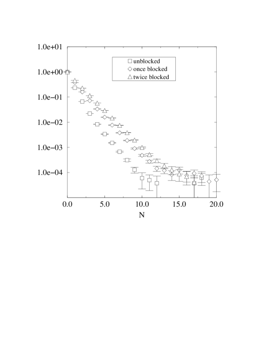
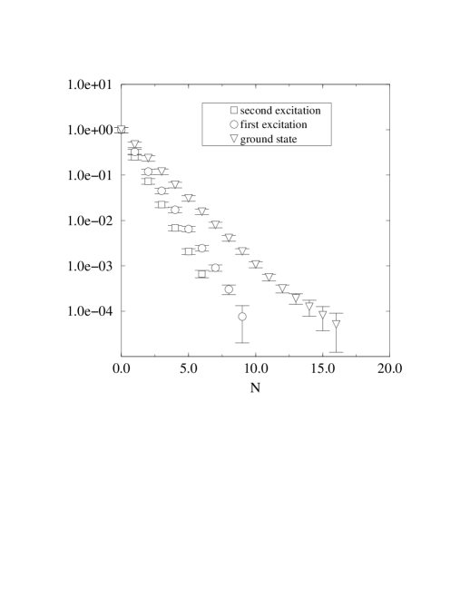
Figure 4: Left: The correlator $G_{F}(T)$ for three different blocking levels in the confinement phase. Right: The diagonalized correlators ${G}_{F_{i}}(T)$ for the three lowest states. Here $\beta_{G}=9$, volume $=42^{3}$, $T=Na$.

	$\exp(-MT)/T^{\alpha}$						$\exp(-MT)/T$				$\exp(-MT)$
$T_{1},T_{2}$	$aM$		$\alpha$		$\chi^{2}$/dof		$aM$		$\chi^{2}$/dof		$aM$		$\chi^{2}$/dof
7, 12	0.	71(11)	-0.	30(84)	0.	63	0.	5366(96)	1.	15	0.	6700(93)	0.	50
6, 12	0.	655(55)	0.	17(35)	0.	58	0.	5217(50)	1.	55	0.	6758(46)	0.	51
5, 12	0.	651(24)	0.	16(14)	0.	63	[huge error]		–		0.	6795(29)	0.	61

Table 1: Comparison of fits to ${G}_{F_{1}}(T)$ in the confinement phase with different functions over various fitting ranges at $\beta_{G}=9$, $L^{2}\cdot L_{T}=42^{3}$.

The situation can be significantly improved upon by performing the diagonalization outlined in the last section. The diagonalized correlation functions corresponding to the three lowest states are shown on the RHS in Fig. 4. In Table 1 we compare the results of fitting different functions to the diagonalized correlator with the lowest mass, ${G}_{F_{1}}(T)$. Acceptable fits using $\exp(-MT)/T$ may be obtained on the late timeslices. However, if one extends the fitting range to earlier time slices the quality of the fit rapidly deteriorates, giving large $\chi^{2}$/dof and/or large errors. On the other hand, we obtain good fits with consistent mass values using a pure exponential $\exp(-MT)$ over a larger range of fitting intervals. Finally, three-parameter fits employing the functional form $\exp(-MT)/T^{\alpha}$ yield values for $\alpha$ that are consistent with zero as well as mass values consistent with those of pure exponential fits. The same behaviour is found for the scalar field correlator and in the Higgs phase as well. The fits for these cases are shown in Table 2.

	$\exp(-MT)/T^{\alpha}$						$\exp(-MT)$
	$aM$		$\alpha$		$\chi^{2}$/dof		$aM$		$\chi^{2}$/dof
${G}_{F_{1}}$, conf.	0.	655(55)	0.	17(35)	0.	58	0.	6758(46)	0.	51
${G}_{\Phi_{1}}$, conf.	0.	3305(53)	-0.	060(40)	0.	53	0.	3228(13)	0.	72
${G}_{F_{1}}$, Higgs	1.	19(15)	-0.	4(5)	0.	34	1.	09(2)	0.	38
${G}_{\Phi_{1}}$, Higgs	0.	05424(8)	0.	0005(6)	–		0.	05428(4)	–

Table 2: Comparison of fitting functions. In each case we consider the same fitting range for both functions. The data are for $\beta_{G}=9$ from the largest lattices considered in each case. The last line corresponds to uncorrelated fits and no $\chi^{2}/dof$ is quoted.

Thus, although there are a few cases where, e.g., a $1/T$ modification of the exponential decay cannot be strictly ruled out based on a finite fitting interval and the value of $\chi^{2}$/dof alone, c.f. Table 1, we have strong numerical evidence that both of the correlators $G_{\Phi}(T)$ and $G_{F}(T)$ decay with a pure exponential $\exp(-MT)$ for large $T$, in both phases. All the following mass estimates have been obtained by fitting a pure exponential to the diagonalized correlation functions ${G}_{\Phi_{i},F_{i}}(T)$.

5.2 Results for the masses

The numerical results for the mass of the “ground state” in the Higgs phase are summarized in lattice units in the first block in Table 3. In [15] it was found that the physical Higgs and W boson masses in the Higgs phase are free from finite volume effects already for rather small lattices, and our choice of lattice sizes is motivated by these findings. As a safeguard, we have performed an explicit check for finite size effects at $\beta_{G}=9$, and Table 3 shows them to be absent. The spatial volumes at $\beta_{G}=12,16$ are larger than merely the scaled up versions of the smallest lattice for $\beta_{G}=9$, so we are confident to have reached the infinite volume limit in those cases as well. Note the very weak exponential decay of the scalar correlator.

	$\beta_{G}$	$\beta_{H}$		$L^{2}\cdot L_{T}$	$aM_{\Phi_{1}}$		$aM_{\Phi_{2}}$		$aM_{F_{1}}$		$aM_{F_{2}}$
Higgs	16	0.	3396	$26^{2}\cdot 36$	0.	04086(4)	–		0.	653(6)	–
phase	12	0.	3418	$24^{2}\cdot 42$	0.	04769(3)	–		0.	836(5)	–
	9	0.	3450	$20^{2}\cdot 36$	0.	05428(4)	–		1.	09(2)	–
				$14^{2}\cdot 36$	0.	05426(5)	–		1.	09(2)	–
conf.	16	0.	3392	$54^{3}$	0.	187(1)(1)	0.	327(14)	0.	397(2)(5)	0.	557(7)
phase				$42^{3}$	0.	187(2)	0.	359(14)	0.	395(5)	0.	559(4)
	12	0.	3411	$42^{3}$	0.	2470(7)	0.	437(7)(12)	0.	516(2)	0.	729(9)(15)
				$30^{2}\cdot 42$	0.	247(1)	0.	448(7)	0.	514(6)	0.	730(8)
	9	0.	3438	$42^{3}$	0.	323(2)	0.	565(4)	0.	677(2)	0.	964(4)
				$24^{2}\cdot 36$	0.	321(2)	0.	557(5)	0.	678(2)	0.	965(6)(5)
pure	16	–		$54^{3}$	–		–		0.	397(3)	0.	566(5)
SU(2)		–		$42^{3}$	–		–		0.	401(4)	0.	566(6)
	12	–		$30^{2}\cdot 42$	–		–		0.	517(7)	0.	744(6)
	9	–		$30^{3}$	–		–		0.	685(3)(7)	0.	960(10)

Table 3: The coefficients of the exponential decay in lattice units. The first error is statistical and the second, where included, is an estimate of systematic effects. In the other cases the systematic errors were estimated to be smaller than the statistical ones.

We remark that in the Higgs phase it was not possible to obtain any reliable information on excited states. In the case of the scalar correlator, the mass of the first excited state appears to be about an order of magnitude larger than that of the ground state. However, the operators of all blocking levels have more than 95% projection onto the ground state, and correspondingly almost no overlap with the first excitation which is hence rather unreliable. In the case of the field strength correlator the effective masses computed from ${G}_{F_{2}}(T)$ do not show a plateau, and correspondingly no fits are possible.

The results for the mass in the confinement phase are shown in the second block in Table 3. Here, we have performed an explicit check for finite size effects for every value of $\beta_{G}$ that we simulated. As is apparent from the table, at least all ground state masses have reached their infinite volume limits. At this point in parameter space we were also able to extract some estimates for the first excitations in the scalar and gauge field channels, which are labelled by $M_{\Phi_{2}}$ and $M_{F_{2}}$, respectively.

Finally, the results for the two lowest states extracted from the field strength correlator in the pure SU(2) theory are given in the third block in Table 3. Note that the numerical values are very close to those found in the confinement phase of the Higgs model. This is not unexpected due to the by now familiar fact [15, 13] that the dynamics of the gauge degrees of freedom in the confinement phase of the Higgs model is rather insensitive to the presence of the scalar fields. The ground state mass for the pure gauge theory has been previously calculated in [4]. In comparing with that work we note that our result is $\sim 5\%$ lower. We ascribe this difference to a better projection achieved by employing the variational technique.

5.3 Continuum limit

$x=0.0239$			$\beta_{G}=9$	$\beta_{G}=12$	$\beta_{G}=16$	$\beta_{G}=\infty$	$\chi^{2}$/dof
Higgs	$\Phi$	$M_{\Phi}/g_{3}^{2}$	0.1221(1)	0.1431(1)	0.1634(2)	–	–
phase		$M^{\prime}_{\Phi}/g_{3}^{2}$	-0.0297(1)	-0.0259(1)	-0.0227(2)	-0.014(3)	2.53
($y=-0.020$)	$F$	$M_{F}/g_{3}^{2}$	2.45(5)	2.51(2)	2.61(3)	–	–
		$M^{\prime}_{F}/g_{3}^{2}$	2.05(5)	2.06(2)	2.12(3)	2.22(8)	1.08
confinement	$\Phi$	$M_{\Phi_{1}}/g_{3}^{2}$	0.727(5)	0.741(2)	0.748(6)	–	–
phase		$M^{\prime}_{\Phi_{1}}/g_{3}^{2}$	0.575(5)	0.572(2)	0.562(6)	0.55(1)	1.12
($y=0.089$)		$M_{\Phi_{2}}/g_{3}^{2}$	1.27(1)	1.31(4)	1.31(6)	–	–
		$M^{\prime}_{\Phi_{2}}/g_{3}^{2}$	1.12(1)	1.14(4)	1.12(6)	1.16(10)	0.16
	$F$	$M_{F_{1}}/g_{3}^{2}$	1.523(5)	1.548(6)	1.59(2)	–	–
		$M^{\prime}_{F_{1}}/g_{3}^{2}$	1.118(5)	1.097(6)	1.09(2)	1.04(3)	0.17
		$M_{F_{2}}/g_{3}^{2}$	2.17(1)	2.19(5)	2.23(3)	–	–
		$M^{\prime}_{F_{2}}/g_{3}^{2}$	1.76(1)	1.74(5)	1.73(3)	1.69(6)	0.03
pure SU(2)	$F$	$M_{F_{1}}/g_{3}^{2}$	1.54(2)	1.55(2)	1.59(1)	–	–
		$M^{\prime}_{F_{1}}/g_{3}^{2}$	1.14(2)	1.10(2)	1.09(1)	1.03(4)	0.2
		$M_{F_{2}}/g_{3}^{2}$	2.16(3)	2.23(2)	2.26(2)	–	–
		$M^{\prime}_{F_{2}}/g_{3}^{2}$	1.76(3)	1.78(2)	1.77(2)	1.79(6)	0.67

Table 4: Masses in continuum units for the largest volumes in Table 3 (see also Figs. 5-7). The primed variables are after the subtraction in eq. (16) and are supposed to have a continuum limit. The linear continuum extrapolation and the corresponding $\chi^{2}/$dof are shown in the two rightmost columns.

Our next task is to examine the scaling behaviour of our results. The data are rewritten in continuum units in Table 4. The scaling of the data with $\beta_{G}$ is shown in Figs. 5-7. The observed slight increase of the mass values with decreasing lattice spacing is attributed to the logarithmic divergence discussed in Sec. 3.1. Unfortunately, the divergence is so weak that in many cases it is not possible to clearly observe it numerically, based on our statistics and $\beta_{G}$-values. In any case, the logarithmic divergence has to be subtracted according to eq. (16) in order to obtain a finite continuum limit. The resulting mass values have been denoted with primes. For the primed quantities we observe rather good scaling consistent with linear $\sim O(a)$ corrections familiar from calculations of the physical particle spectrum of the theory [15]. (Let us note that for some observables the ${\cal O}(a)$ errors could be removed analytically [33], but such a computation has not been made for the mass values obtained from the composite operators in eqs. (1), (2).) The outcome of a linear extrapolation of the mass parameters in $1/\beta_{G}$ to $\beta_{G}=\infty$ is given in Table 4 and constitutes our final result.

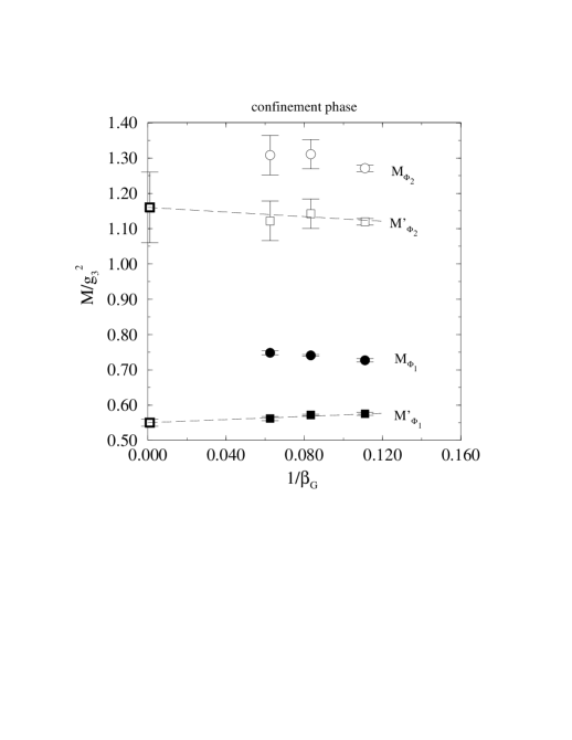
Figure 5: The scaling behaviours of $M_{\Phi_{1}}$, $M_{\Phi_{2}}$ in continuum units. Left: Higgs phase. Right: confinement phase. The linear continuum extrapolations for the primed quantities are also shown. The logarithmic divergence of $M_{\Phi_{1}}$ is so weak that it is not clearly visible in the confinement phase figure for the $\beta_{G}$-values available.

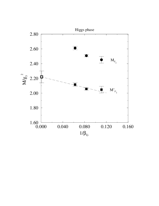
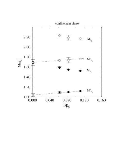
Figure 6: The scaling behaviours of $M_{F_{1}}$, $M_{F_{2}}$ in continuum units. Left: Higgs phase. Right: confinement phase. The linear continuum extrapolations for the primed quantities are also shown.

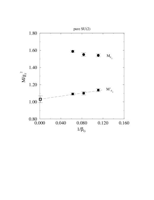
Figure 7: The scaling behaviour of $M_{F_{1}}$ in the pure SU(2) theory. The linear continuum extrapolation for $M^{\prime}_{F_{1}}$ is also shown.

In the Higgs phase one can now compare these results with perturbation theory. The tree-level perturbative $W$ mass at this point is $m_{W}=1.44g_{3}^{2}$. According to eqs. (16), (21), the 1-loop perturbative scalar mass parameter is thus

$${M^{\prime}_{\Phi}}^{\rm pert}=-g_{3}^{2}\frac{3}{16\pi}\ln\left(\frac{m_{W}}{g_{3}^{2}}\right)\sim-0.022g_{3}^{2},$$ (33)

which agrees within $\sim 35\%$ with the full value in Table 4. It should be noted that a large logarithmically divergent 1-loop part has been subtracted in $M^{\prime}_{\Phi}$, so that this agreement is in fact quite good. For the vector mass $M^{\prime}_{F}$ the order of magnitude expectation from the perturbative considerations in Sec. 3.2 was $M^{\prime}_{F}\sim m_{W}$. Indeed we observe agreement in order of magnitude, but quantitatively there is a discrepancy.

6 Discussion

Let us now discuss the physical significance our results may have for the various topics outlined in the introduction. We begin with the application which has immediate physical meaning.

6.1 The Debye mass

An important concept in the phenomenology of high temperature QCD is the static electric screening mass, or the Debye mass $m_{D}$. However, it is a non-perturbative quantity beyond leading order [27]: the expression can be written as

$$m_{D}=m_{D}^{\mbox{\scriptsize LO}}+{Ng_{3}^{2}\over 4\pi}\ln{m_{D}^{\mbox{\scriptsize LO}}\over g_{3}^{2}}+c_{N}g_{3}^{2}+{\cal O}(g^{3}T),$$ (34)

where $m_{D}^{\mbox{\scriptsize LO}}=(N/3+N_{f}/6)^{1/2}gT$ and $N_{f}$ is the number of flavours. The logarithmic part of the ${\cal O}(g^{2})$ correction can be extracted perturbatively [27], but $c_{N}$ and the higher terms are non-perturbative. To allow for a lattice determination, a non-perturbative definition was formulated in [22], employing the dimensionally reduced effective theory of eq. (25), and the further reduction into the pure 3d SU(N) theory, discussed in Sec. 3.3. The statement is that the Debye mass can be determined from the exponential fall-off of the operator odd in $A_{0}^{a}$ which gives the lowest mass value in the theory of eq. (25); or, in terms of the pure SU(2) theory, from the exponential fall-off of an adjoint Wilson line with appropriately chosen adjoint charged operators at the ends such that $M$ obtains its lowest value. The latter is precisely the measurement we have made.

In [22] it was further proposed that one could measure the constant $M$ from the perimeter law of large adjoint charge Wilson loops instead of a single Wilson line, employing essentially eq. (9). As we have discussed, this measurement is in practice much more difficult than a straight Wilson line measurement: so far, it has not been possible to see the saturation of the static potential on the lattice in the adjoint case.

Identifying now $m_{D}$ with $M_{HL}$ in Sec. 3.3, it follows from eqs. (26), (27), (34) that

$$c_{N}=\frac{M_{F_{1}}}{g_{3}^{2}}+\frac{N}{8\pi}\left[\ln\frac{N^{2}}{2\beta_{G}^{2}}-1\right]=\frac{M^{\prime}_{F_{1}}}{g_{3}^{2}}+\frac{N}{8\pi}(\ln 4-1).$$ (35)

Using the value $M^{\prime}_{F_{1}}/g_{3}^{2}=1.03(4)$ from Table 4, we thus obtain $c_{2}=1.06(4)$.

The constant $c_{N}$ has previously been determined directly from the effective theory in eq. (25) for $N=2,3$ in [28], where the physical consequences of the relatively large non-perturbative correction were discussed, as well. In [28], the result for $N=2$ was found to be $c_{2}=1.58(20)$. This is consistent with our result within $\sim(2\ldots 3)\sigma$, but our errorbars are much smaller.

6.2 Constituent masses

In [20] it was suggested that the non-local operators in eqs. (1), (2) would give a gauge-invariant handle on the masses of the light constituents forming the bound states in the confinement phase. The constituent masses are relevant for the bound state model of Ref. [8], as well. In [20] it was further argued that the constituent masses should be consistent with the masses determined from the exponential fall-off of propagators in a fixed Landau gauge [21]. This would then also correspond to the mass value obtained from gap equations in [34].

Let us first recall that within a constituent model, one would write the physical bound state mass $M_{HL}$ as $M_{HL}=M_{H}+M_{L}+E_{B}$, where $M_{H}$ and $M_{L}$ are the masses of the static source and the dynamical charge, respectively, and $E_{B}$ stands for the binding energy. Then in accordance with eq. (26), the mass parameter extracted from our correlators may be written as

$$M=M_{HL}-M_{H}=M_{L}+E_{B}.$$ (36)

This still leaves the definitions of $M_{L}$ and $E_{B}$ open. In particular, it is important to realize that there is a divergence in $M$ and thus in $M_{L}$ or $E_{B}$. The precise way to handle this divergence cannot be decided without a further specification of the constituent model.

In [20] it was suggested that a convenient way of circumventing the problem of the divergence and thus of defining a finite mass value $M^{\prime\prime}$ (which should approximate $M_{L}$ in some constituent models), would be to write $M=M^{\prime\prime}+\delta M$ with a constant $\delta M$, and to require that in the Higgs phase, $M^{\prime\prime}$ corresponds to the physical Higgs or W mass. This of course is only possible if the so defined $M^{\prime\prime}$ has the same parametric dependence on, e.g., the continuum parameter $y$ as the physical masses in the Higgs phase. If such a matching works, then $M^{\prime\prime}$ will differ by a finite constant from the finite mass $M^{\prime}$ defined in eq. (16).

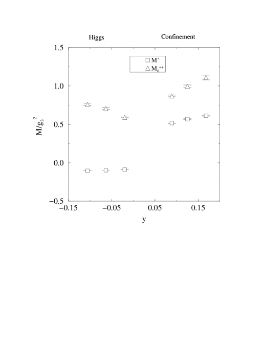
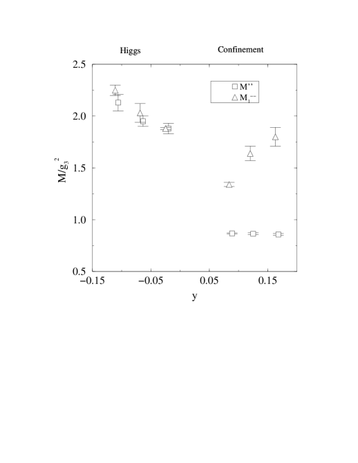
Figure 8: The functional dependence on $y$ at $\beta_{G}=9$. Left: the lowest physical $0^{++}$ state (the Higgs mass in the Higgs phase) and the mass $M^{\prime}$ extracted from $G_{\Phi_{1}}(T)$. Right: the lowest physical $1^{--}$ state (the W-boson in the Higgs phase) and the mass $M^{\prime\prime}$ extracted from $G_{F_{1}}(T)$. The central values of $M^{\prime\prime}$ have been normalized by requiring $M^{\prime\prime}=M_{1^{--}}$ at $y=-0.02$.

The $y$-dependence of the mass parameters extracted from the field correlators is shown in Fig. 8 for $\beta_{G}=9$. Clearly, the matching procedure does not work for the scalar correlator since the Higgs phase result does not behave as the Higgs mass with respect to $y$. The reason is that the signal in the Higgs phase is dominated by the cut-off effect found in perturbation theory, eq. (21). For the vector correlator, on the other hand, the parametric dependence of $M^{\prime\prime}$ in the Higgs phase is found to be close to that of the W mass obtained from the $1^{--}$ operator $V^{a}_{i}(x)\sim{\rm Tr\,}\left(\sigma^{a}\phi^{{\dagger}}(x)U_{i}(x)\phi(x+\hat{i})\right)$, and such a matching can be applied. Setting then

$$M^{\prime\prime}\equiv M^{\prime}_{F_{1}}+Ag_{3}^{2}\;,$$ (37)

A is determined from

$$M^{\prime\prime}(y=-0.020)\equiv m_{W}(y=-0.020)=1.91g_{3}^{2}$$ (38)

to be $A=-0.31g_{3}^{2}$. The $y$-dependence of the $M^{\prime\prime}$ thus obtained is shown in Fig.8 (for $\beta_{G}=9$), together with that of $M_{1^{--}}$. We observe that across the phase transition, $M^{\prime\prime}$ jumps to a smaller value $M^{\prime\prime}(y=0.089)\approx 0.73g_{3}^{2}$ which then remains fairly constant, in contrast to $M_{1^{--}}$. This functional behaviour is similar to that of the W propagator mass in Landau gauge [21], as proposed in [20].

The numerical value of $M^{\prime\prime}$ in the confinement phase may now be compared with those of other mass parameters extracted from lattice simulations. The lightest $0^{++}$ glueball mass is $M_{G}=1.60(4)g_{3}^{2}$ [15]; the fall-off of the W-propagator in Landau gauge in the confinement phase has been determined to be $M^{W}_{LG}=0.35(1)g_{3}^{2}$ [21]. We thus observe that the numerical value of $M^{\prime\prime}$ is about half the glueball mass and twice the propagator mass in Landau gauge. Thus, the conjecture in [20] according to which $M^{\prime\prime}\sim M^{W}_{LG}$, appears not to be satisfied quantitatively.

6.3 Screening

The bound state system of a static source and a dynamical particle in the fundamental or adjoint representation is supposed to correspond to the hadronized final state of the respective static potential at infinite distance, see eq. (9). This permits, in principle, a rough estimate of the screening length $R_{s}$ where the static potential flattens off, given the behaviour of the potential at small distances. The problem is that for the adjoint case, the potential has also been measured up to distances where the screening should show up if this picture is correct [4], but no sign of the screening has been seen. Nevertheless, it might be that the determination of the potential at large distances is less reliable than at small distances [4].

Assuming the potential indeed to be determined reliably only at small distances, one can obtain the following estimates from

$$V(R_{s})\approx 2M.$$ (39)

Since $M$ is scheme dependent, one has to use consistently data from a fixed $\beta_{G}$. For the adjoint case in pure SU(2), our masses are $\sim 5\%$ smaller than measured in [4], but for an order of magnitude estimate this does not matter, and one gets $R_{s}^{-1}\sim 0.2g_{3}^{2}$ from Fig. 8 in [4]. For the fundamental case, we may use the fits made in [8, 35] to the $\beta_{G}=12$ data of [3]:

$$V(R)=C-\frac{3}{8\pi}g_{3}^{2}K_{0}(mR)+\sigma R,$$ (40)

where, corresponding to our confinement phase point, the extrapolated fit parameters have been estimated as $C=0.310g_{3}^{2}$, $m=1.05g_{3}^{2}$ and $\sigma=0.133g_{3}^{4}$ [35]. Using the $\beta_{G}=12$ mass $M_{\Phi_{1}}=0.740g_{3}^{2}$ from Table 4, eq. (39) then gives $R_{s}^{-1}\sim 0.1g_{3}^{2}$ for the fundamental case. Given the uncertainties, these numbers are not to be trusted quantitatively, but it is nevertheless interesting to observe that both the adjoint and the fundamental case give a screening length of the same order of magnitude, and that the corresponding mass scale $R_{s}^{-1}$ is quite small compared with all the correlator masses.

7 Conclusions

In this paper we have reported on the measurements of the expectation values of the operators in eqs. (1), (2) for Wilson lines with various lengths $|x-y|$, on 3d lattices with various lattice sizes and lattice spacings. This allows the extraction of mass signals related to the exponential fall-off of the expectation values, and a study of their scaling behaviour. Subtracting a perturbatively computable logarithmic divergence, we have been able to extrapolate the non-perturbative constant parts to the continuum limit. Apart from the mass signal in the exponential fall-off, we have also measured the asymptotic functional forms of the correlation functions, verifying that they behave according to what is expected for confining theories.

The mass thus measured from eq. (2) for the pure 3d SU(2) theory allows a determination of the leading non-perturbative contribution to the finite temperature Debye mass $m_{D}$ with a method due to Arnold and Yaffe [22]. We obtain a much more precise estimate for $m_{D}$ than has been achieved before: $m_{D}=m_{D}^{\mbox{\scriptsize LO}}+{g_{3}^{2}/(2\pi)}\ln{(m_{D}^{\mbox{\scriptsize LO}}/g_{3}^{2})}+1.06(4)g_{3}^{2}+{\cal O}(g^{3}T)$. The present measurement was made for SU(2) QCD. However, now that our study has proven the practical feasibility of this method, the extension to the realistic SU(3) case is straightforward. The physical significance of the relatively large non-perturbative correction has been discussed in [28].

On the more phenomenological side, the mass signals measured from eqs. (1), (2) are relevant for the composite models proposed to apply in the (symmetric) confinement phase of the SU(2)+Higgs model. This system has been studied as a laboratory for understanding confinement. The main observation based on our data is that, with a definite subtraction procedure, the lattice spacing independent part of the field strength correlator mass is large: it is consistent with about half the glueball mass and twice the mass of the W propagator in Landau gauge.

Finally, we have addressed the question of screening of the static potential. Assuming that the static potential measurements up to date are only reliable at small distances, one obtains both in the pure SU(2) theory and in the SU(2)+Higgs model the rough estimate $1/R_{s}\sim 0.1\ldots 0.2g_{3}^{2}$ for the screening length of adjoint and fundamental representation charges. It is interesting that the mass scale here is much smaller than the other mass scales in the system.

Acknowledgements

We thank M. Gürtler, E.-M. Ilgenfritz and A. Schiller for providing us with data allowing for a check of our code, H. Wittig for routines and useful advice on fitting, and W. Buchmüller, M.G. Schmidt and M. Teper for interesting discussions. The calculations were perfomed on a NEC-SX4/32 at the HLRS Universität Stuttgart.

References

- [1] G. Bali and K. Schilling, Phys. Rev. D 46 (1992) 2636; Phys. Rev. D 47 (1993) 661; Int. J. Mod. Phys. C 4 (1993) 1167; S. Booth et al., Nucl. Phys. B 394 (1993) 509; S. Güsken, in Proceedings of Lattice ’97, in press [hep-lat/9710075].
- [2] C. Michael, Nucl. Phys. B 259 (1985) 58; N.A. Campbell, I.H. Jorysz and C. Michael, Phys. Lett. B 167 (1986) 91; I. Jorysz and C. Michael, Nucl. Phys. B 302 (1987) 448; C. Michael, Nucl. Phys. B (Proc. Suppl.) 26 (1992) 417.
- [3] E.-M. Ilgenfritz, J. Kripfganz, H. Perlt and A. Schiller, Phys. Lett. B 356 (1995) 561; M. Gürtler, E.-M. Ilgenfritz, J. Kripfganz, H. Perlt and A. Schiller, Nucl. Phys. B 483 (1997) 383.
- [4] G.I. Poulis and H.D. Trottier, Phys. Lett. B 400 (1997) 358.
- [5] J. Bricmont and J. Fröhlich, Phys. Lett. B 122 (1983) 73.
- [6] D. Gromes, Phys. Lett. B 115 (1982) 482.
- [7] H.G. Dosch, Phys. Lett. B 190 (1987) 177; H.G. Dosch and Y.A. Simonov, Phys. Lett. B 205 (1988) 339.
- [8] H.-G. Dosch, J. Kripfganz, A. Laser and M.G. Schmidt, Phys. Lett. B 365 (1995) 213; HD-THEP-96-53 [hep-ph/9612450].
- [9] A.D. Giacomo, E. Meggiolaro and H. Panagopoulos, Nucl. Phys. B 483 (1997) 371; M. D’Elia, A.D. Giacomo and E. Meggiolaro, IFUP-TH 19/97 [hep-lat/9705032].
- [10] M. Eidemüller and M. Jamin, HD-THEP-97-49 [hep-ph/9709419].
- [11] G.S. Bali, N. Brambilla and A. Vairo, HD-THEP-97-35 [hep-lat/9709079].
- [12] J. Ambjørn, P. Olesen and C. Peterson, Nucl. Phys. B 240 (1984) 533; D.G. Caldi and T. Sterling, Phys. Rev. Lett. 60 (1988) 2454; R.D. Mawhinney, Phys. Rev. D 41 (1990) 3209; H.D. Trottier and R.M. Woloshyn, Phys. Rev. D 48 (1993) 2290; M. Teper, Phys. Lett. B 289 (1992) 115; Phys. Lett. B 311 (1993) 223.
- [13] O. Philipsen, M. Teper and H. Wittig, HD-THEP-97-37 [hep-lat/9709145].
- [14] K. Kajantie, M. Laine, K. Rummukainen and M. Shaposhnikov, Nucl. Phys. B 466 (1996) 189; Nucl. Phys. B 493 (1997) 387.
- [15] O. Philipsen, M. Teper and H. Wittig, Nucl. Phys. B 469 (1996) 445.
- [16] K. Kajantie, M. Laine, K. Rummukainen and M. Shaposhnikov, Phys. Rev. Lett. 77 (1996) 2887.
- [17] P. Ginsparg, Nucl. Phys. B 170 (1980) 388; T. Appelquist and R. Pisarski, Phys. Rev. D 23 (1981) 2305.
- [18] K. Kajantie, M. Laine, K. Rummukainen and M. Shaposhnikov, Nucl. Phys. B 458 (1996) 90; E. Braaten and A. Nieto, Phys. Rev. D 53 (1996) 3421; A. Jakovác and A. Patkós, Nucl. Phys. B 494 (1997) 54.
- [19] E. Eichten, Nucl. Phys. B (Proc. Suppl.) 4 (1988) 170.
- [20] W. Buchmüller and O. Philipsen, Phys. Lett. B 397 (1997) 112.
- [21] F. Karsch, T. Neuhaus, A. Patkós and J. Rank, Nucl. Phys. B 474 (1996) 217.
- [22] P. Arnold and L. Yaffe, Phys. Rev. D 52 (1995) 7208.
- [23] H.G. Evertz, V. Grösch, J. Jersák, H.A. Kastrup, T. Neuhaus, D.P. Landau and J.-L. Xu, Phys. Lett. B 175 (1986) 335.
- [24] M. Gürtler, E.M. Ilgenfritz, A. Schiller and C. Strecha, in Proceedings of Lattice’97, in press [hep-lat/9709020].
- [25] K. Farakos, K. Kajantie, K. Rummukainen and M. Shaposhnikov, Nucl. Phys. B 442 (1995) 317; M. Laine, Nucl. Phys. B 451 (1995) 484; M. Laine and A. Rajantie, Nucl. Phys. B, in press [hep-lat/9705003].
- [26] N.G. van Kampen, Phys. Rep. 24 (1976) 171.
- [27] A.K. Rebhan, Phys. Rev. D 48 (1993) R3967; Nucl. Phys. B 430 (1994) 319.
- [28] K. Kajantie, M. Laine, K. Rummukainen and M. Shaposhnikov, Nucl. Phys. B, in press [hep-ph/9704416]; K. Kajantie, M. Laine, J. Peisa, A. Rajantie, K. Rummukainen and M. Shaposhnikov, Phys. Rev. Lett. 79 (1997) 3130 [hep-ph/9708207].
- [29] K. Fabricius and O. Haan, Phys. Lett. B 143 (1984) 459.
- [30] A.D. Kennedy and B.J. Pendleton, Phys. Lett. B 156 (1985) 393.
- [31] B. Bunk, Nucl. Phys. B (Proc. Suppl.) 42 (1995) 566.
- [32] M. Teper, Phys. Lett. B 183 (1987) 345.
- [33] G.D. Moore, Nucl. Phys. B 493 (1997) 439; McGill-97-23 [hep-lat/9709053].
- [34] W. Buchmüller and O. Philipsen, Nucl. Phys. B 443 (1995) 47.
- [35] A. Laser, PhD thesis, Heidelberg 1996 (unpublished).