The $\eta^{\prime}$ Meson with Staggered Fermions

Abstract

We have computed the $\eta^{\prime}$-pseudoscalar octet mass splitting using staggered fermions on both dynamical and quenched gauge configurations. We have used Wuppertal smeared operators to reduce excited state contributions. We compare our results with the theoretical forms predicted by partially quenched chiral perturbation theory in the lowest order. Using lattice volumes of size $16^{3}\times 32$ with $a^{-1}=2$GeV we obtain results consistent with the physical $\eta^{\prime}$ mass. We also demonstrate that the flavor singlet piece of the $\eta^{\prime}$ mass comes from zero modes of the Dirac operator.

I INTRODUCTION

By now there have been dozens of calculations of the masses of most of the light hadrons using lattice QCD. However, until recently the $\eta^{\prime}$ meson received only scant attention, in large part because of the relative difficulty of the calculation: the disconnected contraction which gives the $\eta^{\prime}$ propagator its special character is an order of magnitude more expensive to compute. A previous study [1] made a first study of the $\eta^{\prime}$ two-point function using quenched Wilson fermions, finding a vertex of the right size to explain the $\eta^{\prime}$ mass. Here we improve the situation in several ways, by using staggered fermions which have better chiral properties, by going closer to the chiral limit, and most importantly by using gauge configurations with dynamical fermions. The authors of the earlier study also took a step toward confirming the conventional wisdom that the $\eta^{\prime}$ receives its special mass from instantons by sorting their gauge fields into bins of topological charge. Here we take the further step of examining the contribution of topological zero modes of the Dirac operator to the $\eta^{\prime}$ propagator. The results again confirm the lore that this is the mechanism by which the $\eta^{\prime}$ gets its mass.

The $\eta^{\prime}$ meson is one of the more intriguing strongly interacting particles. Although it is the lightest flavor singlet pseudoscalar, it is too heavy to be the Goldstone boson of a $U(1)$ axial symmetry, as was pointed out by Weinberg [2] long ago. With the emergence of QCD it was understood that this $U(1)$ symmetry is actually anomalous, so that one should not expect an associated Goldstone boson. A qualitative understanding of the mechanism behind the $\eta^{\prime}$ mass was provided in the framework of the large $N_{c}$ expansion. When $N_{c}\rightarrow\infty$  [3, 4], $U(1)$ axial symmetry is restored and gives rise to $\eta^{\prime}-\pi$ degeneracy. This degeneracy is lifted by the presence of virtual quark loops (Fig  1) in the $\eta^{\prime}$ propagator which are suppressed by one power of $1/N_{c}$. Infinite iteration of these quark antiquark annihilation diagrams gives rise to a geometric series for the Euclidean $\eta^{\prime}$ propagator. Defining the correlator $\langle\eta^{\prime}(t)\eta^{\prime}(0)\rangle$ one can write its Fourier transform as

$$G_{\eta^{\prime}}\,\,\,\,\,\sim\,\,\,\,\,\frac{1}{p^{2}\,\,+\,\,m_{8}^{2}}\,\,-\,\,\frac{m_{0}^{2}}{p^{2}\,\,+\,\,m_{8}^{2}}\,\,+\,\,\frac{1}{p^{2}+m_{8}^{2}}\,m_{0}^{2}\,\frac{1}{p^{2}+m_{8}^{2}}\,m_{0}^{2}\frac{1}{p^{2}+m_{8}^{2}}\,\,+{}\cdots$$ (1)

where $m_{8}^{2}$ is the average of the square of the octet masses and $m_{0}^{2}$ is the strength of the flavor singlet interaction. Summing the geometric series shifts the pole from $m_{8}^{2}$ to $m_{0}^{2}+m_{8}^{2}$. Thus

$$\langle\eta^{\prime}(t)\eta^{\prime}(0)\rangle\,\,\,\,\sim\,\,\,\,\frac{1}{p^{2}\,\,+\,\,m_{8}^{2}\,\,+m_{0}^{2}}$$

In an $SU(3)$ symmetric world, one would write

$$m_{\eta^{\prime}}^{2}=m_{0}^{2}+m_{8}^{2}$$ (2)

$m_{8}^{2}$ vanishes in the chiral limit while $m_{0}^{2}$ does not. Taking $m_{8}^{2}=(4m_{K}^{2}+3m_{\pi}^{2}+m_{\eta}^{2})/8$ and substituting the experimentally measured values for $m_{\eta^{\prime}}$, $m_{K}$, $m_{\pi}$ and $m_{\eta}$, one obtains $m_{0}=860{\rm MeV}$.

The large $N_{c}$ approximation also gives the qualitative understanding that this $m_{0}$ is linked to instantons. To leading order in $1/N_{c}$ one finds the Witten-Veneziano formula

$$m_{0}^{2}=\frac{2\,N_{f}\chi}{f_{\pi}^{2}}$$ (3)

where $N_{f}$ is the number of flavors, $\chi$ is the topological susceptibility and $f_{\pi}$ is the pion decay constant. In the real world, taking the number of active light flavors to be three, one needs $\chi$ of order $(185{\rm MeV})^{4}$ to explain the $\eta^{\prime}$. Lattice QCD calculations of the quenched topological susceptibility (e.g. [5]) do indeed give results in this range. Thus modulo concerns over $1/N_{c}$ corrections, definitions of topological charge, setting the quenched scale etc., one could claim that lattice calculations give a quantitatively correct indirect determination of $m_{0}$.

II Direct Lattice Calculation of $m_{0}$

Lattice QCD offers the challenge of calculating $m_{0}^{2}$ directly from the $\eta^{\prime}$ propagator without resort to any argument based on large $N_{c}$. The quantity of interest is the two point function $\langle{\eta^{\prime}}(x){\eta^{\prime}(y)}$, where the simplest choice for the interpolating field $\eta^{\prime}(x)$ is $\overline{Q}(x){\gamma}_{5}\,Q(x)$. As illustrated in figure  2, there are two types of contractions to take into account: (i) the single quark loop connected diagram which contributes to flavor-singlet and flavor non-singlet mesons alike, and (ii) the disconnected diagram which appears only for the flavor singlet $\eta^{\prime}$. As in the previous lattice studies [1, 6, 7, 8], we find it convenient to define the ratio $R(t)$ of the disconnected two loop amplitude to the connected one loop amplitude

$$R(t)=\frac{\langle\eta^{\prime}(t)\eta^{\prime}(0){\rangle}_{disc}}{\langle\eta^{\prime}(t)\eta^{\prime}(0){\rangle}_{conn}}$$ (4)

Noting the asymptotic behavior

$${\langle{\eta^{\prime}(0)\eta^{\prime}(t)}\rangle\over\langle{\pi(0)\pi(t)}\rangle}\rightarrow{Z^{\prime}\exp(-m_{\eta^{\prime}}t)\over Z\exp(-m_{\pi}t)}$$ (5)

one sees that in full unquenched QCD the ratio $R(t)$ asymptotes to $1-B\exp(-\Delta mt)$, where B is a constant and $\Delta m=m_{\eta^{\prime}}-m_{8}$. This statement assumes that there are equal numbers of dynamical and valence flavors and $m_{dyn}=m_{val}$. If one has differing numbers of valence and dynamical fermions, as we do when using staggered fermions, then one needs to rescale the connected diagram of fig 2 by $N_{f}/N_{v}$, and the disconnected diagram by $(N_{f}/N_{v})^{2}$. Therefore $R(t)$ takes the form

$$R(t)=\frac{N_{v}}{N_{f}}\,\,[1\,\,-\,\,B\exp(-\Delta mt)]$$ (6)

On quenched configurations, the absence of closed quark loops means that the basic vertex is not allowed to iterate, and equation 1 is truncated after the first two terms. Thus in the quenched approximation, there is a double pole in the $\eta^{\prime}$ propagator. This means for the zero spatial momentum state, $R(t)$ rises linearly with the slope $\frac{m_{0}^{2}}{2m_{8}}\,t$.

$$R(t)=const.+\frac{m_{0}^{2}}{2m_{8}}\,t$$ (7)

We have used staggered fermions, both dynamical and quenched configurations and local and Wuppertal smeared operators for the extraction of $m_{\eta^{\prime}}$. We also study the dynamical flavor dependence of $m_{\eta^{\prime}}$ and have derived the expected theoretical forms for the ratio using partially quenched chiral perturbation theory ($PQ\chi PT$) so as to enable comparison of our results with theory. In section 3, we review the basic concepts of $PQ\chi PT$ [9] and derive expressions for $R(t)$. In section 4, we describe details pertaining to the parameters of the simulation and the Wuppertal smearing procedure. In section 5 we discuss the results obtained from our simulation and compare with the theoretical predictions of section 2.

III RATIO from $PQ\chi PT$

Bernard and Golterman [10, 9] have developed a technique for constructing an effective chiral theory for quenched and partially quenched QCD. The basic idea in this approach is based on the observation that if a scalar quark ($\tilde{q}$) is added to the QCD Lagrangian, then the scalar determinant can cancel the quark determinant. For concreteness, if we assume there are $N_{v}$ quarks of masses $m_{i}(i=1,2..N_{v})$, then adding $k$ pseudoquarks of masses $m_{j}(j=1,2..k)$ such that $m_{j}=m_{i}$ would mean that first $k$ quarks are quenched and the remaining $N_{v}-k$ unquenched. The low energy effective chiral theory then describes interactions among all kinds of boundstates, including the ordinary pions as well as unphysical states containing scalar quarks. The reader is referred to  [10, 9] for discussion regarding the form of the Lagrangian and its symmetry properties. For the purposes of this paper, it is sufficient to write down the Green’s function in momentum space in the basis of the states corresponding to $\overline{u}u$, $\overline{d}d$ and their pseudoquark counterparts:

$$G_{ij}=\frac{{\delta}_{ij}{\epsilon}_{i}}{p^{2}+M_{i}^{2}}-\frac{m_{0}^{2}}{(p^{2}+M_{i}^{2})(p^{2}+M_{j}^{2})F(p^{2})}$$ (8)

where

$$F(p^{2})=1+m_{0}^{2}\sum_{d=k+1}^{N_{v}}\frac{1}{p^{2}+M_{d}^{2}},$$ (9)

$M_{i}^{2}$ is the square of the meson mass composed of quark flavor $i$ and

$${\epsilon}_{i}=\cases{+1&{$1\leq i\leq N_{v}$}\cr-1&{$N_{v}+1\leq i\leq N_{v}+k$}}$$ (10)

In the above, the term proportional to $\alpha$, the momentum dependent self-interaction of $\eta^{\prime}$ has been neglected. It can be reinstated any time by the substitution $m_{0}^{2}\rightarrow m_{0}^{2}+{\alpha}^{2}p^{2}$. When $m_{i}=m_{j}$ the first term is simply the neutral meson propagator in the absence of flavor singlet interactions. The second term is obtained from summing the infinite geometric series obtained by iterating the flavor singlet interaction. When simulating with staggered fermions on $N_{f}=2$ dynamical configurations, the variables $N_{v}$ and $k$ take the values 4 and 2 respectively. Specifically, when all the valence flavors have the same mass $m_{val}$ and all the dynamical flavors have mass $m_{dyn}$ but $m_{val}\neq m_{dyn}$, (in a typical simulation this situation would arise if one were simulating with staggered fermions on dynamical configurations) the Green’s function above takes the form,

$$G_{ii}=\frac{1}{p^{2}+M_{i}^{2}}-\frac{m_{0}^{2}\,\,\,(p^{2}+M_{d}^{2})}{(p^{2}+M_{i}^{2})^{2}\,\,(p^{2}+M_{d}^{2}+N_{f}m_{0}^{2})}$$ (11)

It is straightforward to go over to configuration space, project each term on to zero spatial momentum state and then take the ratio of the second term to the first term. Doing so we obtain

$$R(t)=\,\,\frac{N_{v}}{N_{f}}\,[\,At\,\,-\,\,B\exp(-\Delta mt)\,\,+\,\,C]$$ (12)

where

$$A=\frac{(m_{d}^{2}-m_{8}^{2})(m_{d}^{2}-m_{\eta^{\prime}}^{2})}{(m_{8}^{2}-m_{\eta^{\prime}}^{2})2m_{8}},$$ (13)

$$B=\frac{m_{8}(m_{d}^{2}-m_{\eta^{\prime}}^{2})^{2}}{m_{\eta^{\prime}}(m_{8}^{2}-m_{\eta^{\prime}}^{2})^{2}},\\$$ (14)

$$C=\frac{(m_{d}^{2}-m_{\eta^{\prime}}^{2})}{(m_{8}^{2}-m_{\eta^{\prime}}^{2})}\,\left[\frac{(m_{d}^{2}-m_{8}^{2})}{2m_{8}^{2}}\,+\,\frac{(m_{d}^{2}-m_{8}^{2})}{(m_{8}^{2}-m_{\eta^{\prime}}^{2})}+1\right],$$ (15)

$$m_{8}^{2}\equiv M_{i}^{2}=M_{j}^{2},\,\,\,m_{d}^{2}\equiv M_{d}^{2}\,\,\,\,\rm{and}$$ (16)

$$m_{\eta^{\prime}}^{2}=m_{d}^{2}+N_{f}\,m_{0}^{2}.$$ (17)

As a check we note that eqn 12 contains the expression in eqn 6 and eqn 7 as appropriate limits. When $m_{8}=m_{d}$, one obtains eqn 6 with $B=m_{8}/m_{\eta^{\prime}}$, and in the limit $m_{d}\rightarrow\infty$, $N_{f}\rightarrow 0$ one obtains eqn 7 with the intercept equal to $\frac{m_{0}^{2}}{2m_{8}^{2}}$. We have ratio data on quenched and $N_{f}=2$ configurations. Our ratio data on $N_{f}=2$ configurations can be further divided into $m_{val}=m_{dyn}$ and $m_{val}\neq m_{dyn}$. Quenched and $m_{val}=m_{dyn}$ data can be subjected to both one and two parameter fits thus enabling comparison between the predictions of the theory and “experiment”. Likewise, a similar comparison is possible from both one and four parameter fit to $m_{val}\neq m_{dyn}$ data.

IV SIMULATION DETAILS

A Ensemble

The propagators required for computing the disconnected and the connected amplitude were computed on configurations of size $16^{3}\times 32$. The statistical ensemble used and the valence quark masses at which the simulation was performed are shown in table I. The dynamical configurations were borrowed from Columbia while the quenched configurations were generated on the Cray T3D at Ohio Supercomputer Center(OSC). By design, the ensembles listed in table I have the same inverse lattice spacing of about $2{\rm GeV}$ obtained from $m_{\rho}$. The values of $m_{val}$ on the quenched configurations were chosen 10% higher than those on the dynamical configurations, in order to bring the corresponding values of $m_{8}$ into more precise agreement. The staggered propagators were computed by invoking the conjugate gradient method using sets of processors ranging from 16 to 64 nodes of the Cray T3D at OSC and Los Alamos’s Advanced Computer Laboratory with a sustained performance of 45 Mflops per node.

B Propagators

The pseudoscalar operator that creates or destroys an $\eta^{\prime}$ in the staggered formalism is $\overline{Q}{\gamma}_{5}\otimes IQ$. It is a distance 4 operator in which the quark and the antiquark sit at the opposite corners of the hypercube. We put in explicit links connecting the quark and the antiquark across the edges of the hypercube and averaged over all the 24 possible paths to make the operator gauge invariant. As was mentioned earlier, the two point correlation function of this operator yields both the connected one loop and the disconnected two loop amplitude of fig 2. Two propagators need to be computed for calculating the one loop amplitude. One propagator was calculated using a delta function source with a local random phase ${\eta}_{x}=\exp(i\theta(x))$ at each spatial site and for each color on time slices $t=1$ and $t=2$. When averaged over all noisy samples, the noise ${\eta}_{x}$ satisfies $\langle{\eta}_{x}{\eta}_{y}^{{\dagger}}\rangle={\delta}_{xy}$. Translating the noisy source at each site (made gauge invariant by putting in links) a hypercubic distance 4 and putting in the phase appropriate for the $\eta^{\prime}$ operator, the second propagator was calculated. Transporting the source and calculating the anti-propagator separately is the price paid due to the non locality of the staggered flavor singlet operator. For each configuration we took two noise samples with the lattice doubled in the time direction.

Very few lattice calculations of $m_{\eta^{\prime}}$ exist because of the difficulty involved in getting good signals for the disconnected amplitude using reasonable computer time. We have addressed this problem by using a noisy source like the one used for the connected amplitude but placed on all sites of the lattice. Then we solve $(\hbox to0.0pt{\,/\hss}D+m)\phi=\eta$ and estimate the quark propagator as $G_{xy}=\langle m{\phi}_{x}{\phi}_{y}^{{\dagger}}\rangle$ with $|x-y|$ even. The distance 4 staggered flavor singlet operator that we use satisfies this criterion. At this point it should be mentioned that there also exists a distance 3 staggered flavor singlet operator for which the the appropriate estimator of $G_{xy}$ is $\langle{\eta}_{x}^{{\dagger}}{\phi}_{y}\rangle$. This channel did not yield good signals for the the pseudofermion propagators, and we did chose not to examine it further. In any case, $\langle m{\phi}_{x}{\phi}_{y}^{{\dagger}}\rangle$ is a better estimator than $\langle{\eta}_{x}^{{\dagger}}{\phi}_{y}\rangle$ since the fluctuations in the former go as ${\langle\overline{\chi}\chi\rangle}^{2}$ while those for the latter are of the order $\langle\overline{\chi}\chi\rangle/m_{val}$ where ${\langle\overline{\chi}\chi\rangle}$ is the condensate. For the range of light quark masses chosen in this simulation, ${\langle\overline{\chi}\chi\rangle}$ lies between 0 and 1, thus making ${\langle\overline{\chi}\chi\rangle}^{2}$ significantly less than $\frac{\langle\overline{\chi}\chi\rangle}{m_{val}}$. We used 16 noise samples per configuration, again on a doubled lattice.

C Wuppertal Smearing

Fig 3 shows the ratio $R(t)$ on quenched and dynamical configuration ($N_{f}=2,m_{dyn}=0.01$) using local interpolating fields. Since the disconnected data is noisy, the ratio data is only useful for the first few time slices where the contribution due to excited states is non-negligible. Smeared operators reduce the contributions from excited states and enable a more reliable extraction of ${\Delta}m$ from the available data.

We used the Wuppertal smearing technique [11] in which one obtains an exponentially decaying bound state wavefunction from solving

$$(-{\nabla}^{2}[U]+{\kappa}^{2})\phi(x)={\delta}_{x,0}$$ (18)

where ${\kappa}^{2}$ is a parameter that can be tuned to control the spread of the wavefunction. On the lattice, for staggered fermions and to make the smearing procedure gauge invariant, the operator ${\nabla}^{2}$ takes the form

$${\nabla}^{2}[U] \rightarrow \frac{1}{2}\sum_{\mu=1}^{3}U_{\mu}(x)\,\,U_{\mu}(x+\mu)\,\delta_{x^{\prime},x+2\mu}+\,\,U_{\mu}^{\dagger}(x-\mu)\,U_{\mu}^{\dagger}(x-2\mu)\delta_{x^{\prime},x-2\mu}\,\,-\,\,2{\delta}_{x^{\prime},x}$$ (19)

We experimented with different values of ${\kappa}^{2}$ and determined that the critical value occurred near ${\kappa}^{2}=-0.64$. The values of ${\kappa}^{2}$ that are relevant to this study are those near the critical value since this corresponds to a maximum spread in the wavefunction without losing the exponential behavior. The form of the wavefunction obtained on one of the $N_{f}=2(m_{dyn}=0.01)$ configurations is shown in fig 4.

For this study, one propagator of the connected correlator was calculated with the source smeared to a fixed radius corresponding to ${\kappa}^{2}=-0.6$ and a point-like sink. This was tied to five different anti-propagators with point-like source but smeared at the sink end corresponding to different values of ${\kappa}^{2}$ (see fig 5). Thus the smeared valence propagators that we have calculated correspond to the set of correlators shown in table II.

A typical effective mass plot obtained on $N_{f}=2$, $m_{dyn}=0.01$ configuration at $m_{val}=0.01$ is shown in fig 6 for the correlator LL. Since decrease in ${\kappa}^{2}$ increases the spread in the wavefunction, among the 5 correlators shown in table II, $C_{5}$ is expected to perform the best which is evident by comparing fig 6 and fig 7. We also defined the correlator

$$\langle\cos\theta\,\overline{Q}(x)Q(x)+\sin\theta\,\overline{Q}_{w4}(x)Q(x)\rangle$$ (20)

which amounts to taking the linear combination

$$({\cos}^{2}\theta\,LL+{\sin}^{2}\theta\,C_{5}+2\cos\theta\,\sin\theta C_{1})$$ (21)

We determined the angle $\theta$ for which the value of the effective mass on $t=1$ was the lowest and this corresponded to $\theta=.797\pi$. We denote this linear combination of correlators as $LLC_{5}$ and it is clear from fig 7 that it is slightly better than $C_{5}$.

To calculate the corresponding disconnected contributions of the correlators listed in  II, the sink end of the pseudofermion propagator ($\phi^{\prime}$) was smeared to 4 different radii corresponding to ${\kappa}^{2}=-0.5,\,\,-0.53,\,\,-0.56$ and $-0.6$ (see fig 5). Accordingly, the quark propagator was obtained from the estimator $G_{xy}^{\prime}=\langle m{\phi}_{x}^{\prime}{\phi}_{y}^{{\dagger}}\rangle$.

Fig 8 compares the ratio plot with and without smearing on dynamical configurations. In the initial time slices both the data are different but they begin to coincide after a few time slices as they should.

V RESULTS

In the plot of figure 9, the different curves represent the fit to the ratio data obtained from the various configurations listed in table I. For $N_{f}=2$ the points shown correspond to $m_{val}=m_{dyn}$ while for the quenched data the points correspond to $m_{val}=0.011$. The quenched data is fit linearly according to equation 7 with both the intercept and the slope as free parameters. The dynamical data is fit according to equation 6 with both $m_{\eta^{\prime}}$ and $B$ as free parameters. A remarkable observation that is to be gleaned from this graph is that the ratio data is distinctly different for different numbers of dynamical flavors and in accordance with the predicted theoretical form. If nothing else, this observable is clearly able to distinguish quenched from dynamical configurations.

Our values of $m_{8}$ calculated on quenched and $N_{f}=2$ dynamical configurations are plotted as a function of the valence quark mass in fig 10. We note that at this finite lattice spacing, $m_{8}$ does not quite vanish in the chiral limit. This is a consequence of our taking the flavor singlet ($\gamma_{5}\otimes I$) pion as opposed to the special (flavor $T_{5}$) staggered pion. Of course even for our pion, the intercept should vanish in the continuum limit.

From the linear fit to the quenched data for $m_{val}=0.011,\,\,\,0.022\,\,\,{\rm and}\,\,\,0.033$, we extract $m_{0}^{2}$ from the slope. A plot of $m_{0}^{2}$ against $m_{val}$ and the extrapolation to the zero quark mass is shown in fig 11. $m_{0}^{2}$ increases with decreasing quark mass and does not vanish in the chiral limit. Smearing has lowered the value of the intercept obtained in the zero quark mass limit, bringing it closer to the real world value.

Two parameter fits, according to eqn 6, of the dynamical $m_{val}=m_{dyn}$ data yields $\Delta m$ and hence $m_{\eta^{\prime}}$. Extrapolating the values of $m_{\eta^{\prime}}$ so extracted, we find that it does not vanish in the chiral limit (fig 12). As seen in quenched case, the values of $m_{\eta^{\prime}}$ both at finite and zero quark mass due to the correlator $LLC_{5}$ are lower than the corresponding points due to the local correlator LL. Errors quoted on the ratio data and all the mass values are obtained by doing a single elimination jackknife.

We could not obtain stable 4 parameter fits to our $m_{val}\neq m_{dyn}$ data. The known theoretical forms for the ratio obtained from lowest order $PQ\chi PT$ were used for one parameter fit of the $m_{val}\neq m_{dyn}$ and $m_{val}=m_{dyn}$ data. Fig 13 shows the theoretical fit obtained for $m_{val}=0.02$ on $N_{f}=2$ , $m_{dyn}=0.01$ configuration using smeared operators. One parameter fit to the data obtained with local operators gave reasonable ${\chi}^{2}$ only if the fit range began from $t\geq 3$. This suggests that the local data is heavily contaminated with excited states since the formulae derived in section 2 hold for asymptotic times. Doing a similar job for $m_{val}=0.03$ data and extrapolating the value of $m_{\eta^{\prime}}$ obtained from both to the chiral limit we obtain $m_{\eta^{\prime}}(N_{f}=3)=876\pm 16{\rm MeV}$ which is remarkably consistent with the value obtained from fully quenched and dynamical data (table III).

A one parameter fit to $m_{val}\leq m_{dyn}$ data did not yield reasonable ${\chi}^{2}$. However, for the $m_{val}=m_{dyn}$ data, it was possible to extract the deviation from the lowest order $PQ\chi PT$ as determined by the observable $Z^{\prime}/Z$, the ratio of the residues for creating ${\eta^{\prime}}$ and ${\eta}$.

$$\frac{Z^{\prime}}{Z}=\frac{{\mid\langle 0\mid\eta^{\prime}(0)\mid\eta^{\prime}\rangle\mid}^{2}}{{\mid\langle 0\mid\eta(0)\mid\eta\rangle\mid}^{2}}$$ (22)

In $PQ\chi Pt$, this ratio is 1 based on the assumption $f_{\eta^{\prime}}=f_{\eta}$. Therefore, in $PQ\chi PT$ as shown in section 2, the parameter B in eqn 6 equals $\frac{m_{8}}{m_{\eta^{\prime}}}$ instead of $\frac{m_{8}Z^{\prime}}{m_{\eta^{\prime}}Z}$. From the 2 parameter fit to the $m_{val}=m_{dyn}$ data one can then determine the ratio $Z^{\prime}/Z$. The values we extract for $Z^{\prime}/Z$ are plotted as a function of $m_{val}$ in fig 14 both for smeared and local data. It can be seen that the data prefer to be 20-30% above unity which is typically the size of higher order chiral and $O(1/N_{c})$ corrections.

In the analysis so far, we have neglected the effect of momentum dependence of $m_{0}^{2}$, ie. we had been working in a theory with $\alpha$, the coefficient of the kinetic energy term of $\eta^{\prime}$ in the chiral Lagrangian [9], set to zero. $\alpha$ is expected to be a small quantity, contributing only at the next to leading order in a combined expansion in $1/N_{c}$ and quark mass [10]. Including $\alpha$ simply shifts the strength of the flavor singlet interaction vertex from $m_{0}^{2}$ to $m_{0}^{2}+{\alpha}^{2}m_{8}^{2}$. While the form of $R(t)$ remains the same as before for all the three cases, the coefficients of the time dependent terms and the constants become functions of two unknown parameters, $m_{0}^{2}$ and $\alpha$. For the quenched case, we obtain

$$R(t)=\frac{(m_{0}^{2}-\alpha\,m_{8}^{2})\,t}{2\,m_{8}}\,\,+\,\,\frac{(m_{0}^{2}+\alpha\,m_{8}^{2})}{2\,m_{8}^{2}}$$ (23)

It is clear from the above formula that the value of $m_{0}^{2}$ is shifted by a small amount at finite quark mass and indeed this is borne out true by the quenched ratio data when fit to the above form. We see 10%-15% downward shift in the the values of $m_{0}^{2}$ obtained from the slope and the intercept of the fit at non zero quark mass. When extrapolated to the chiral limit, the value of $m_{0}^{2}$ is left unaffected (within quoted errors in table III) by the presence of the momentum dependent interaction term. The statistical errors associated with the extracted values of $\alpha$ are rather large. Our results for $\alpha$ for each quark mass is shown in table  IV.

On dynamical configurations, the presence of a non zero $\alpha$ is reflected in the expression for $m_{\eta^{\prime}}$. It now takes the form

$$m_{\eta^{\prime}}^{2}=\frac{N_{f}\,m_{0}^{2}+m_{8}^{2}}{1+N_{f}\,\alpha}$$ (24)

The natural quantity that is extracted from fitting the dynamical $m_{val}=m_{dyn}$ data with equation 6 is $m_{\eta^{\prime}}$ which cannot be used to determine both $m_{0}^{2}$ and $\alpha$ independently.

VI FERMIONIC ZEROMODES

As reassuring as it may be that our lattice results correctly reproduce the physical $\eta^{\prime}$ mass, the calculation itself does not illuminate the precise mechanism by which the $\eta^{\prime}$ gets its special mass. The conventional lore, as quantified by the Witten-Veneziano formula, associates $m_{0}$ with the fluctuations in the topological charge. In a previous study, Kuramashi et al. tried to verify this relation by calculating the topological susceptiblity of their gauge configurations and using it to calculate $m_{0}$. They obtain a value that is higher than the experimantal number. Here we chose to illuminate the question by focusing directly on the fermionic zero-modes which are associated with the topological charge of a gauge configuration via the index theorem.

In the continuum, integrating the anomaly equation gives the relation

$$Q=m\,{\rm tr}\,({\gamma}_{5}\,S_{F})$$ (25)

where $S_{F}$ is the fermion propagator. Resolving the propagator in a sum over eigenmodes of $\hbox to0.0pt{\,/\hss}D$, and noting that all modes with nonzero eigenvalue come in conjugate pairs, one gets the index theorem:

$$Q=n_{+}-n_{-}.$$ (26)

Here $n_{+}$ ($n_{-}$) is the number of positive (negative) chirality zeromodes. If the $\eta^{\prime}$ is particularly sensitive to the topological charge of a configuration, then one must also expect it to be sensitive to the presence or absence of fermionic zeromodes.

On the lattice, both sides of the index equation are slightly distorted. The flavor singlet $\gamma_{5}$ does not exactly anticommute with $\hbox to0.0pt{\,/\hss}D$, so the trace of $\gamma_{5}S_{F}$ cannot be collapsed into a trace in the zeromode sector alone. Further, there are no exact zeromodes, nor is there an exact definition of the topological charge. Nevertheless, if we are sufficiently close to the continuum, something like the conventional picture should obtain.

We have taken a look [13] by constructing the lowest few eigenmodes of $\hbox to0.0pt{\,/\hss}D$ on both the quenched and dynamical ($N_{f}=2$, $m_{dyn}=.01$) ensembles of gauge fields. We use the method of subspace iterations as described in ref. [12]. This algorithm obtains the eigenmodes of $\hbox to0.0pt{\,/\hss}D^{2}$ by minimization of the Ritz functional

$$\mu(X_{e})={\mathop{\rm Tr}}\left[(X^{{\dagger}}_{e}X_{e})^{-1}(X^{{\dagger}}_{e}(-{\hbox to0.0pt{\,/\hss}D}^{2})X_{e})\right].$$ (27)

Here $X_{e}$ is the rectangular matrix of $m$ eigenvectors. The subscript indicates we only need the solution on the even sites; full eigenmodes of ${\hbox to0.0pt{\,/\hss}D}$ can then be easily reconstructed on the odd sites. We found it necessary to modify the algorithm slightly, periodically reorthogonalizing the columns of the block vector $X_{e}$. With the modes themselves in hand one can then construct approximate propagators and ask how well these small eigenvalue modes reproduce the full answers we obtain by conventional means.

In figure 15 we show the contribution to the topological charge coming from the eigenmodes in one typical dynamical configuration. In terms of the eigenmodes, equation 25 takes the form

$$Q=m\sum_{\lambda}{\frac{{\psi}_{\lambda}^{{\dagger}}\,{\gamma}_{5}\,{\psi}_{\lambda}}{i{\lambda}+m}}.$$ (28)

As can be seen, after the first few modes, the sum quickly saturates to the full answer obtained by averaging over many copies of pseudofermion noise.

That this behavior is typical of the whole ensemble can be seen in the scatter plot of figure 16, which plots the eigenvalue, $\langle\gamma_{5}\rangle$ pairs collected on all configurations. The largest contributions to the trace evidently come from the smallest eigenmodes. We conclude that even at this finite lattice spacing, the index theorem is perfectly recognizable.

It is only natural to extend the analysis further to calculate the $\eta^{\prime}$ disconnected correlator, which is proportional to the fluctuations in the topological charge and is given by $\langle{\rm tr}({\gamma}_{5}\,G(x,x)){\rm tr}({\gamma}_{5}\,G(y,y))\rangle$. The result of calculating this using the available eigenmodes is shown in figure 17. It is evident that the first few modes give essentially the full answer.

One may wonder if the chiral modes may be used to successfully reproduce other hadronic correlators as well. In terms of the eigenmodes, the approximate propagator is of the form

$$G_{xy}\approx\sum_{\lambda}{\psi_{\lambda}(x)\psi^{{\dagger}}_{\lambda}(y)\over i\lambda+m}$$ (29)

Figure 18 answers this question for the case of the Goldstone pion. Even with the full 32 modes, the pion propagator is off by a large factor both in its overall normalization, and in its mass parameter. Evidently the $\eta^{\prime}$ is special in that it is exquisitely sensitive to the lowest handful of modes.

VII CONCLUSIONS

We have computed both the quenched flavor singlet vertex $m_{0}$ and the full dynamical $\eta^{\prime}$ mass, finding agreement with the experimental numbers. Since the statistical errors are relatively large we have not attempted to pin down the systematic errors, e.g. from finite lattice spacing and from the neglect of $\eta$-$\eta^{\prime}$ mixing. Our results both confirm our conventional understanding of the $\eta^{\prime}$ in QCD and show that lattice QCD can be a useful tool in this difficult sector. We have also shown that unlike other hadron correlators, the $\eta^{\prime}$ propagator is particularly sensitive to the presence of fermionic zeromodes. This result supports the connection of the $\eta^{\prime}$ to topology.

TABLE I.: The Statistical Ensemble

$N_{f}$	$m_{dyn}$	$\beta$	$N_{samp}$	$m_{val}$
0	$\infty$	6.0	83	0.011
				0.022
				0.033
2	0.01	5.7	79	0.01
				0.02
				0.03
2	0.015	5.7	50	0.01
				0.015
2	0.025	5.7	34	0.01
				0.025

TABLE II.: Smeared valence operators. The spin/flavor is ${\gamma}_{5}\otimes I$ in each case.

	Contraction		${\kappa}^{2}$ at source	${\kappa}^{2}$ at sink
LL	$\overline{Q}(x)Q(x)$	$\overline{Q}(0)Q(0)$	no smearing	no smearing
$C_{1}$	$\overline{Q}(x)Q(x)$	$\overline{Q}_{w4}(0)Q(0)$	-0.6	no smearing
$C_{2}$	$\overline{Q}_{w1}(x)Q(x)$	$\overline{Q}_{w4}(0)Q(0)$	-0.6	-0.5
$C_{3}$	$\overline{Q}_{w2}(x)Q(x)$	$\overline{Q}_{w4}(0)Q(0)$	-0.6	-0.53
$C_{4}$	$\overline{Q}_{w3}(x)Q(x)$	$\overline{Q}_{w4}(0)Q(0)$	-0.6	-0.56
$C_{5}$	$\overline{Q}_{w4}(x)Q(x)$	$\overline{Q}_{w4}(0)Q(0)$	-0.6	-0.6

TABLE III.: $m_{\eta^{\prime}}(N_{f}=3)$ in the chiral limit.

	Quenched	Dynamical ($m_{dyn}=m_{val}$)
	(MeV)	(MeV)
LL	1156(95)	974(133)
${\rm LLC_{5}}$	891(101)	780(187)

TABLE IV.: $\alpha$ from the quenched ratio data.

$m_{val}\,a$	LL	$LLC_{5}$
0.011	-1.7496(2321)	-0.2988(2091)
0.022	-0.8475(1301)	-0.1431(1195)
0.033	-0.4645(910)	-0.0399(702)

FIG. 1.: Virtual quark loops in the $\eta^{\prime}$ propagator

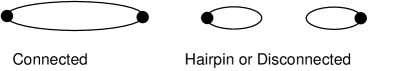
FIG. 2.: Contributions to $\eta^{\prime}$ correlator

FIG. 3.: Ratio using local operators.

FIG. 4.: Wavefunction from Wuppertal smearing.

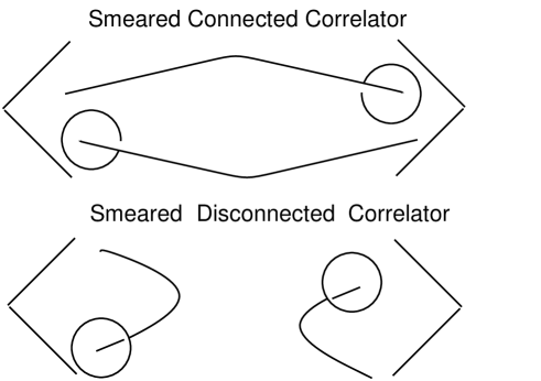
FIG. 5.: Correlators from smeared operators.

FIG. 6.: Effective mass plot for $m_{8}$ with LL correlator.

                          

FIG. 7.: Effective mass plot with $C_{5}$ and $LLC_{5}$ correlators.

FIG. 8.: Dynamical ratio from local and smeared operators.

FIG. 9.: Flavor dependence of $R(t)$.

                 

FIG. 10.: $m_{8}^{2}$ vs $m_{val}$ on $N_{f}=0$ and $N_{f}=2$ configurations.

FIG. 11.: Chiral extrapolation of quenched $m_{0}^{2}$.

FIG. 12.: Chiral extrapolation of ${m_{\eta^{\prime}}}^{2}$ from $N_{f}=2$ configurations.

FIG. 13.: One parameter fit to $R(t)$ with $m_{val}=0.02$ and $m_{dyn}=0.01$.

FIG. 14.: $Z^{\prime}/Z$ vs. $m_{val}$.

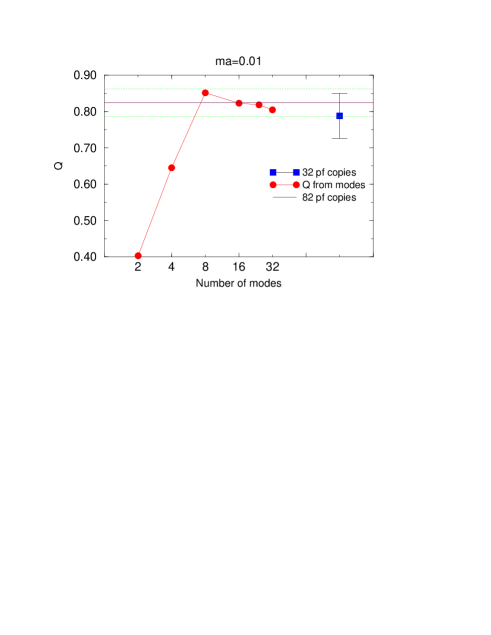
FIG. 15.: Topological charge on a typical dynamical configuration

FIG. 16.: Above:$\langle{\Gamma}_{5}\rangle$ on the dynamical ensemble. Below: Fluctuations in $\langle{\Gamma}_{5}\rangle$.

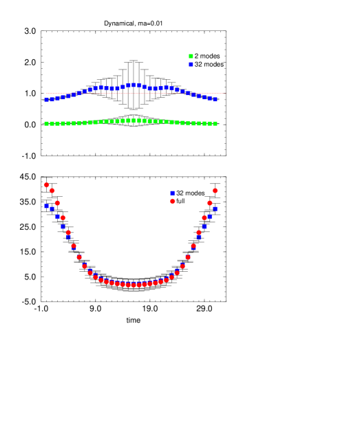
FIG. 17.: Below: Comparison of the two loop amplitudes. Above: Ratio of the full two-loop amplitude to that calculated with modes.

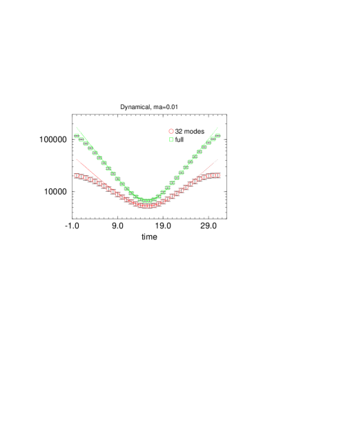
FIG. 18.: Pion propagator on dynamical ensemble at $ma=0.01$.

REFERENCES

- [1] Y. Kuramashi et al., Phys. Rev. Lett. 72 (1994) 3448.
- [2] S. Weinberg, Phys. Rev. D11 (1975) 3583.
- [3] E. Witten, Nucl. Phys. B156 (1979) 269.
- [4] G. Veneziano, Nucl. Phys. B159 (1979) 213.
- [5] B. Alles, M. D’Elia and A. Di Giacomo, Nucl. Phys. B494 (1997) 281.
- [6] G. Kilcup, J. Grandy and L. Venkataraman, Nucl. Phys. (Proc. Supp.) 47 (1996) 358.
- [7] M. Masetti et al., Nucl. Phys. B480 (1996) 381.
- [8] H. Thacker et al., hep-lat/9608110.
- [9] C. Bernard and M. Golterman, Phys. Rev. D49 (1994) 486.
- [10] C. Bernard and M. Golterman, Phys. Rev. D46 (1992) 853.
- [11] S. Guesken, Nucl. Phys.(Proc. Supp.) 17 (1990) 361.
- [12] B. Bunk, Nucl. Phys.(Proc. Supp.) 53 (1997) 987.
- [13] L. Venkataraman and G. Kilcup, Proceedings of Lattice 97.