Advances in the Determination of Quark Masses

Abstract

Significant progress has been made in the determination of the light quark masses, using both lattice QCD and sum rule methods, in the last year. We discuss the different methods and review the status of current results. Finally, we review the calculation of bottom and charm masses.

1 Introduction

One of the primary goals of phenomenology is to determine the fundamental parameters of the standard model. Of these, the five quark masses $m_{u},m_{d},m_{s},m_{c},m_{b}$ are amongst the least well known, and cannot be measured in experiments. They have to be inferred from the pattern of the observed hadron spectrum (chiral perturbation theory ($\chi$PT), HQET, and lattice QCD approaches) or from the study of 2-point correlation functions (sum rules and lattice QCD approaches). This review is mainly an assessment of lattice QCD results, however we shall also summarize the results obtained using $\chi$PT and sum-rules. In particular we shall evaluate the extent to which these methods agree with each other and discuss recent developments in each.

$\chi$PT relates pseudoscalar meson masses to $m_{u}$, $m_{d}$, and $m_{s}$. However, due to the presence of an overall unknown scale in the chiral Lagrangian, $\chi$PT can predict only two ratios amongst the three light quark masses [2, 3, 4]

	Lowest order	Next order
$2m_{s}/(m_{u}+m_{d})$	$24.2-25.9$	$24.4(1.5)$  .
$m_{u}/m_{d}$	$0.55$	$0.553(43)$ .

These ratios have been calculated neglecting the Kaplan-Manohar symmetry [5]. This is justified by assuming that the higher order terms are small as discussed in [4]. These ratios, when combined with an absolute value determined from sum-rules completed the “standard” scenario. The status of sum-rule estimates, as of 1996 was, $2\hbox{$\overline{m}$}\equiv m_{u}+m_{d}=9.4(1.8){\rm MeV}$ [6] and $m_{s}=126(13){\rm MeV}$ [7], evaluated in the $\overline{\rm MS}$ scheme at scale $\mu=2{\rm GeV}$. These, combined with $\chi$PT ratios, give the standard estimates (in ${\rm MeV}$)

Input	$m_{u}$	$m_{d}$	$\overline{m}$	$m_{s}$
$m_{s}$	3.7(1.0)	6.7(0.8)	5.2(0.6)	-
$\overline{m}$	3.3(1.3)	6.1(1.1)	-	115(23) .

These values are consistent with observed spectra, $i.e.$ one can explain the electromagnetic splittings, and the SU(3) breaking in the mesons and in the baryon octet and decuplet without recourse to large non-linear terms in $m_{q}$. The limitation of this combined analysis, especially of the absolute numbers, is that there are no independent checks as the quark masses enter in phenomenology only in combination with other unknown quantities like the quark condensate. In the last year there has been considerable activity in sum-rule analyses, and we shall summarize these in Section 7.

Lattice QCD is a relative newcomer. Last year a major step forward was taken in the understanding and quantification of systematic errors. An analysis of the global data consolidated the lattice predictions of significantly lower light quark masses [8, 9]

	Quenched	$N_{f}=2$
$(m_{u}+m_{d})/2$	$3.4(7)$	$\sim 2.7$ ${\rm MeV}$
$m_{s}$	$100(31)$	$\sim 70$ ${\rm MeV}$ .

The lattice results for the quenched theory were considered reliable as three different discretizations of the Dirac action, Wilson, clover, and staggered, gave results consistent after extrapolation to the continuum limit. The unquenched estimates ($N_{f}=2$ theory results) were preliminary. The main message was that including two flavors of dynamical quarks lowers the quenched estimates by $\sim 20\%$.

The abbreviation “1996 data” will be used to denote lattice data analyzed in [8]. This will be used as the benchmark against which progress will be measured. Other reviews and references to lattice results can be found in [10, 11, 12]. The main sources of uncertainty in the lattice estimates we shall explore are (i) the extrapolation of the data to the continuum limit, (ii) the matching constants between the lattice and continuum scheme, and (iii) the effect of sea quarks (corrections due to quenching). We are happy to report that there has been significant progress in all three areas in the last year.

2 Lattice Approach: From Spectroscopy

Lattice calculations need to determine four independent quantities to predict the three light quark masses. The fourth is needed to fix the lattice spacing $a$. To distinguish between $m_{u}$ and $m_{d}$, it is necessary to include electromagnetic corrections. This can be done by including a U(1) field in the simulations [13], however, since the effect is small compared to statistical and systematic errors, current lattice simulations have, for the most part, neglected it. Thus, this review is restricted to the determination of the isospin symmetric combination $\overline{m}$.

A brief outline of how the three quantities $\overline{m}$, $m_{s}$, and $a$ are determined from the light hadron spectrum is as follows. Using $\chi$PT as the guiding principle, one writes down the most general expansion of hadron masses in terms of quark masses $m_{1},m_{2},m_{3}$,

$$M_{\pi}^{2}a^{2}\mskip-9.0mu = \mskip-9.0muA_{\pi}+B_{\pi}a(m_{1}+m_{2})/2+\ldots$$

$$M_{\rho}a\mskip-9.0mu = \mskip-9.0muA_{\rho}+B_{\rho}a(m_{1}+m_{2})/2+\ldots$$

$$M_{\Sigma^{+}}a\mskip-9.0mu = \mskip-9.0muA_{\Sigma^{+}}+4Fam_{1}+2(F-D)am_{3}+\ldots$$

$$M_{\Delta}a\mskip-9.0mu = \mskip-9.0muA_{\Delta}+B_{\Delta}a(m_{1}+m_{2}+m_{3})/3+\ldots,$$ (1)

where for brevity we shall use $\pi,\rho,\Delta$ to denote members of the pseudoscalar and vector octet and the baryon decuplet respectively. Chiral symmetry implies $A_{\pi}\equiv 0$. We leave it as a free parameter in the fits – it gives a measure of the uncertainty in the zero of the mass scale.

The simplest scenario is that there are no higher order corrections to Eq. 1. Then, any triplet like $B_{\pi},A_{\rho},B_{\rho}$ (or equivalently $B_{\pi},A_{\Delta},B_{\Delta}$) can be used to determine $\overline{m}$, $m_{s}$, and $a$. For example, using the first set, the quark masses are determined as

$$\hbox{$\overline{m}$}=\frac{M_{\pi}^{2}}{B_{\pi}a^{-1}}\,;\,m_{s}=\frac{2(M_{K^{*}}-A_{\rho}a^{-1})}{B_{\rho}}-\hbox{$\overline{m}$}\,,$$ (2)

and the scale from $M_{\rho}$ by solving the quadratic

$$A_{\rho}(\frac{1}{a})^{2}-M_{\rho}(\frac{1}{a})+B_{\rho}\frac{M_{\pi}^{2}}{B_{\pi}}=0\,.$$ (3)

Similar relations exist for other choices of observables. The scale $1/a$ can, in fact, be taken from other observables like $M_{n}$, $M_{\Delta}$, $f_{\pi}$, string tension, $r_{0}$, or the $1P-1S$ splitting in quarkonia. We choose $a(M_{\rho})$ based on its ready availability and statistical quality of $M_{\rho}$ versus $M_{n}$, $M_{\Delta}$ and $f_{\pi}$ data. Different choices lead to different results, an unavoidable uncertainty inherent in the quenched approximation. We shall refer to this hadron spectroscopy method by the abbreviation HS.

If linearity were exact, or the exact expansions in Eq. 1 were known, then any single set, like the pseudoscalar octet masses, could be used to fix both $\hbox{$\overline{m}$}a$ and $m_{s}a$. There is no a priori reason to assume that the higher order chiral corrections are negligible. In fact, using $M_{\pi}/M_{K}$ or $M_{\eta}/M_{K}$ give different estimates for $m_{s}/\hbox{$\overline{m}$}$ in lowest order $\chi$PT. Also, present lattice data show non-linearities in the pseudoscalar and vector meson data if a sufficiently large range of quark masses is chosen [14, 15]. However, these non-linearities are small, and are very hard to detect in the typical range $m_{s}/3<m_{q}<2m_{s}$ used to extract quark masses. Thus, unless otherwise stated, we have used just linear fits in the chiral extrapolation.

The more serious problem facing quenched simulations is that this range cannot be extended easily to much smaller quark masses due to the presence of artifacts called quenched chiral logs. (For recent reviews and references to this body of work see [11, 16].) These terms, which are not present in the normal chiral expansion, are singular in the limit $m_{q}\to 0$ and are a consequence of the fact that, in the quenched approximation, the $\eta^{\prime}$ propagator has a single and a double pole. The approach, therefore, has been to fit the quenched data in this limited range, where these artifacts are small, keeping just the normal chiral expansion. The quenching error is then the change in these coefficients as sea quark effects are added.

Finally, a test of the combined uncertainties due to quenching, and chiral and $a\to 0$ extrapolations is that quark masses extracted using different observables should all give the same results. We shall discuss the extent to which this is satisfied by comparing $m_{s}$ extracted from $M_{K}$ with that from $M_{K^{*}}$ or $M_{\phi}$ (labeled $m_{s}(M_{K})$, $m_{s}(M_{K^{*}})$, $m_{s}(M_{\phi})$ respectively). Most of the figures we shall present will be for $\overline{m}$, however, note that due to the linear approximation in Eq. 1, the result for $m_{s}(M_{K})$ is $\equiv 25.9\hbox{$\overline{m}$}$. $m_{s}(M_{\phi})$ gives an independent estimate, but the statistical signal in the data for vector state masses is not as good as for pseudoscalars. This will be evident from the figures we show for $m_{s}(M_{\phi})$.

2.1 Definition of quark mass

For staggered fermions, the fits in Eq. 1 are made as a function of the bare quark mass input into the simulations. For Wilson-like fermions, we define light quark masses by

$$am_{bare}=\log(1+(\frac{1}{2\kappa}-\frac{1}{2\kappa_{c}}))$$ (4)

where $\kappa_{c}$ is the critical value of the hopping parameter at which the lattice pion mass vanishes. (Reference [8] used $am_{bare}=1/2\kappa-1/{2\kappa_{c}}$, which is consistent to $O(a)$. This change leads to differences of a few percent.) So, compared to staggered fermions, Wilson like fermions require the determination of an additional quantity $\kappa_{c}$. The need to calculate $\kappa_{c}$ can be avoided by using the Ward Identity method described below. From $m_{bare}$, the $\overline{\rm MS}$ mass is obtained as

$$m_{\overline{\rm MS}}=Z_{m}m_{bare}$$ (5)

where $Z_{m}=1/Z_{S}$ is the matching factor between $\overline{\rm MS}$ and lattice schemes. Since this factor turns out to be large at 1-loop, its reliability has to be checked by non-perturbative methods.

2.2 Ward Identity (WI) method

For Wilson like fermions, one can extract quark masses from pseudoscalar mesons by using the axial vector ward identity

$$Z_{A}\partial_{\mu}A_{\mu}(x)=(m_{1}+m_{2})Z_{P}P(x)+\ldots$$ (6)

where $A_{\mu}$ is the appropriate flavor non-degenerate bare axial current $\overline{\psi}\gamma_{\mu}\gamma_{5}\psi$, $P$ is the corresponding pseudoscalar density $\overline{\psi}\gamma_{5}\psi$, and the $Z$’s are the corresponding renormalization constants. The dots represent discretization corrections, whose size depends on the order to which improvement of the action and operators has been carried out. The renormalized quark masses are then given by the ratio of 2-point functions

$$(m_{1}+m_{2})=\frac{Z_{A}}{Z_{P}}\frac{\langle\partial_{\mu}A_{\mu}(x)J(0)\rangle}{\langle P(x)J(0)\rangle}+\ldots$$ (7)

where $J$ is any operator that couples to pions. The advantage of this $WI$ method is that $\kappa_{c}$ does not enter into the calculation. The limitation is that only the pseudoscalar sector is tested.

3 Details of the analysis of World Data

Different groups have their own favorite ways of doing the fits, and of dealing with the two major sources of systematic errors, the extrapolation to the continuum limit and the determination of $Z$’s. Consequently, the same data analyzed by different groups can lead to slightly different estimates of quark masses. Since we wish to do a global analysis, we have attempted to minimize these relative differences. We start with the data for pseudoscalar and vector mesons as a function of quark masses and $g^{2}$, and redo the analysis to extract $A_{\pi},B_{\pi},A_{\rho},B_{\rho}$. For the physical masses we use $M_{\pi}=135$ MeV, $M_{\rho}=770$ MeV, $M_{K}=495$ MeV, $M_{K^{*}}=894$ MeV, and $M_{\phi}=1020$ MeV. (Ref. [8] used $M_{\pi}=137$, thus $\overline{m}$ quoted there is about 3% higher.) This still leaves two sources of uncertainty. (i) The difference in lattice sizes and the subjective bias in fits made to extract hadron masses. This we check by comparing data from different collaborations. (ii) The statistical correlations in the data. These require knowledge of the covariance matrix which is not available in most cases.

To convert the lattice mass to a continuum scheme like $\overline{\rm MS}$, we require the calculation of either $Z_{S}$ in both lattice and continuum renormalization scheme (HS method), or of $Z_{A}$ and $Z_{P}$ (WI method). For these matching factors 1-loop results have been used in the past. Now, non-perturbative estimates are becoming common. The calculation of the Lepage-Mackenzie $\alpha_{s}$, “horizontal” matching between the lattice and continuum schemes in the perturbative approach, details of the error analysis, and the evolution in the continuum are the same as in [8]. The relevant formula for the 2-loop evolution needed with the 1-loop matching is [17]

$${m(Q)\over m(\mu)}=\bigg{(}{g^{2}(Q)\over g^{2}(\mu)}\bigg{)}^{\gamma_{0}/2\beta_{0}}\ \bigg{(}1+{g^{2}(Q)-g^{2}(\mu)\over 16\pi^{2}}J\bigg{)}\,,$$ (8)

where $J=(\gamma_{1}\beta_{0}-\gamma_{0}\beta_{1})/2\beta_{0}^{2}$. From this the renormalization group invariant mass $\widehat{m}$ is defined as

$$\widehat{m}=m(\mu)\bigg{(}{2\beta_{0}g^{2}(\mu)\over 16\pi^{2}}\bigg{)}^{-\gamma_{0}/2\beta_{0}}\ \bigg{(}1-{g^{2}(\mu)\over 16\pi^{2}}J\bigg{)}.$$ (9)

This evolution in the continuum or the conversion to $\widehat{m}$ introduce no new lattice uncertainty.

Now we briefly highlight two important developments by the APE and ALPHA collaborations that overcome the uncertainty introduced by the perturbative matching.

The APE collaboration has carried through non-perturbative determination of the lattice $Z$’s [18] using the chiral Ward identity method [19, 20]. At present non-perturbative estimates of all the necessary lattice $Z$’s for all the actions we discuss are not known. As these become available, the uncertainty in using the 1-loop relations will be removed. We shall discuss the impact of the known $Z$’s on current data.

The ALPHA Collaboration has initiated a very successfully non-perturbative program to improve the discretization of the Dirac action, fermionic operators, and their renormalization constants [21]. The improvement they propose over APE’s chiral Ward Identity method for determining the $Z^{\prime}s$ is to eliminate making any connection with a continuum scheme by directly computing the renormalization group independent quark mass. The essential steps in their method are (i) calculate the renormalized quark mass using the WI method at some infrared lattice scale ($Z_{P}$ and $Z_{A}$ are also calculated non-perturbatively in the Schrödinger functional scheme), (ii) evolve this result to some very high scale using the step scaling function calculated non-perturbatively, and (iii) at this high scale, where $\alpha_{s}$ is small, make contact with lattice perturbation theory to define $\widehat{m}$. This non-perturbatively calculated $\widehat{m}$ is scheme independent, thus subsequent conversion to a running mass in some scheme and at some desired scale can be done in the continuum using the most accurate versions of the scale evolution equations [22]. No data for $\widehat{m}$ has yet been released. The status of this approach has been reviewed by Lüscher at this conference [21].

4 Quenched Wilson fermion results

The Wilson formulation of the Dirac action is the simplest and has been the most commonly used in numerical simulations until very recently. Its disadvantage is that discretization errors and violations of chiral symmetry begin at $O(a)$. Nevertheless, a 1996 compilation of the world data for quark masses [8] showed that an extrapolation to the continuum limit can be made keeping only the lowest order corrections, giving

$$\overline{m} = 3.4(7){\rm MeV}[1+1.3(2){\rm GeV}\ a]$$

$$m_{s}(M_{\phi}) = 94(27){\rm MeV}[1+1.9(7){\rm GeV}\ a].$$ (10)

The surprise was the size of the $O(a)$ errors. The typical size of the slope in $a$ obtained in the extrapolation of other observables like $M_{\rho},f_{\pi},\ldots$ is a few hundred MeV, so the $1.2-1.7{\rm GeV}$ values needed to be understood.

Significant progress in this sector has been made by the recent high statistics, large lattice calculations by CP-PACS which have been reviewed by T. Yoshie in [23]. They have provided four new data points on lattices of size $\geq 3$ fermi. The new data are shown in Fig. 1. To highlight the statistical improvement we show data at $\beta=6.0$ from the next best calculation (with respect to both statistics and lattice size) [15]. The data from both HS and WI methods are well fit by just a linear correction, and extrapolate to roughly the same value

$$\overline{m} = 4.1(1){\rm MeV}[1+0.49{\rm GeV}\ a]\qquad{\rm HS}$$

$$\overline{m} = 4.2(1){\rm MeV}[1-0.32{\rm GeV}\ a]\qquad{\rm WI}.$$ (11)

The CP-PACS data, therefore, gives a significantly smaller slope and a larger value for $\overline{m}$.

In Fig. 1 we also show the 1996 fit. The change in the slope is due to a pivot about $\beta\approx 5.9$. Further analysis based on the CP-PACS data shows that the three APE points at $\beta=6.3,6.4$, that biased the 1996 fits towards lower values of $\overline{m}$, are not compatible within errors with CP-PACS; the estimates of both $B_{\pi}$ and $a$ differ. Our conclusion is that these data should not be used in “modern analyses”.

     

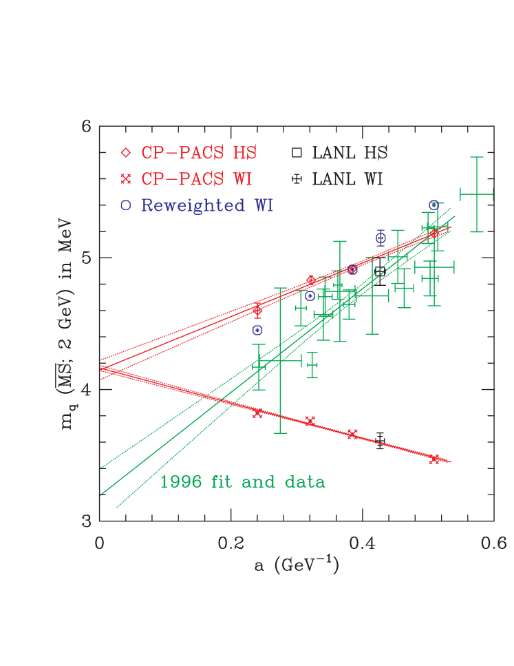
Figure 1: Linear extrapolation of $\overline{m}$ versus $a(M_{\rho})$ for Wilson fermions using HS and WI methods. The 1996 data and fit are shown in green.

The CP-PACS collaboration also calculate $m_{s}$ using both $M_{K}$ and $M_{\phi}$ ($M_{\phi}$ and $M_{K^{*}}$ give consistent results). The new data are shown in Fig. 2. The data show that $m_{s}(m_{K})$ and $m_{s}(M_{\phi})$ are different even after extrapolation to the continuum limit, as was the case in the 1996 data,

$$m_{s}\,(M_{\phi}) = 139(11){\rm MeV}[1+0.47{\rm GeV}\ a]$$

$$m_{s}(M_{K}) = 107(2){\rm MeV}[1+0.49{\rm GeV}\ a].$$ (12)

Assuming that this difference is not an artifact of statistical errors or due to the uncertainty in the extrapolation, it could be due either to quenching, or to the failure of the assumption of linearity in the chiral fits. In that case one will need unquenched data to resolve this issue. Meanwhile, we consider this difference as one of the remaining systematic errors. These estimates for $m_{s}$ are larger than those reported in 1996. The reasons for the change are the same as for $\overline{m}$.

     

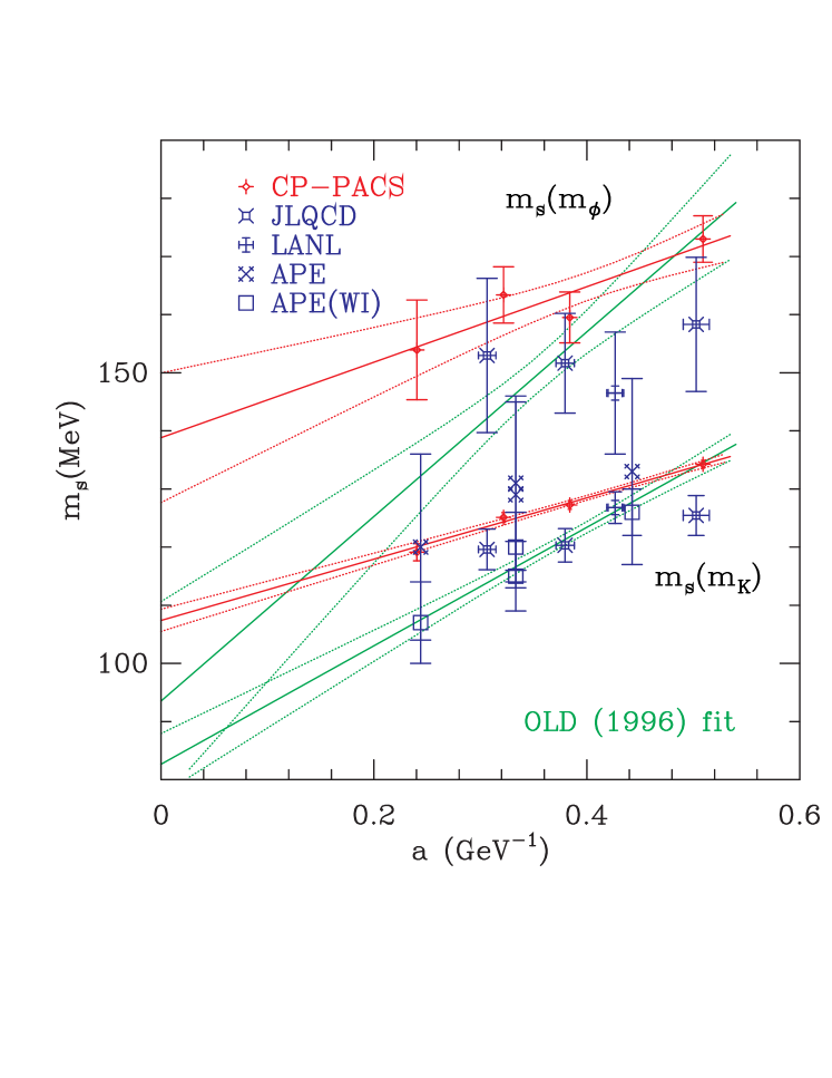
Figure 2: Linear extrapolation of $m_{s}(M_{K})$ and $m_{s}(M_{\phi})$ versus $a(M_{\rho})$ for Wilson fermions. The 1996 fits are shown in green for comparison.

The second important contribution of the CP-PACS analysis is the reconciliation of the HS and WI methods. The data, and the fits shown in Fig. 1 indicate that the difference between the two methods at finite $a$ is due to different $O(a)$ discretization errors. Giusti et al. [18] argue that this difference is due to the failure of the 1-loop $Z$’s. We have therefore reanalyzed the CP-PACS/LANL WI data using the non-perturbative $Z_{A},Z_{P}$ calculated by Giusti et al. (we interpolated or extrapolated the Giusti et al. results to other $\beta$ linearly). These reweighted points are plotted using the symbol octagon in Fig. 1. What is remarkable is the agreement between non-perturbative WI and perturbative HS data around $\beta=6.1$, and the change in the slope, $i.e.$ the slope switches sign and ends up being even larger than that for HS with 1-loop $Z$’s! This equality of HS and WI data around $\beta=6.1$ is consistent with the findings of Giusti et al. [18] as discussed in section 4.3. What the APE data cannot expose is the slope in $a$ from simulations at just $\beta=6.0$ and $6.2$. We would also like to point out that $Z^{non-pert}/Z^{pert}$ typically decreases rapidly with $\beta$ as, for example, in Table 1. Hence, if the 1-loop $Z_{m}$ turns out to be an underestimate, then correcting for it will increase the slope of the HS data as well. Thus, the issue of the size of the slope, and of the final extrapolated value will be resolved soon, once the non-perturbative estimates of $Z_{m}$ are made available [18].

4.1 Clover Action

One way to reduce/remove the large $O(a)$ corrections in the Wilson formulation, and thus improve the reliability of the $a=0$ extrapolation, is to simulate the Sheikholeslami-Wohlert (SW or clover) action. In the last couple of years a number of calculations have been done using this action. Unfortunately, different calculations use different values of $C_{SW}$: (i) tree-level value $C_{SW}=1$, (ii) tree-level Tadpole Improved (TI), (iii) 1-loop tadpole improved, and (iv) non-perturbative $O(a)$ improved. To get a feel for the effects of tuning $C_{SW}$, we first show in Fig. 3 the data for $\overline{m}$ for different values of $C_{SW}$ as a function of $a$. The data at $\beta=6.0$ show that as $C_{SW}$ is increased, $\overline{m}$ decreases and $a$, as determined from $M_{\rho}$, increases. The expectation is that as $\beta\to\infty$, the ordering should stay the same, only the spread should decrease.

     

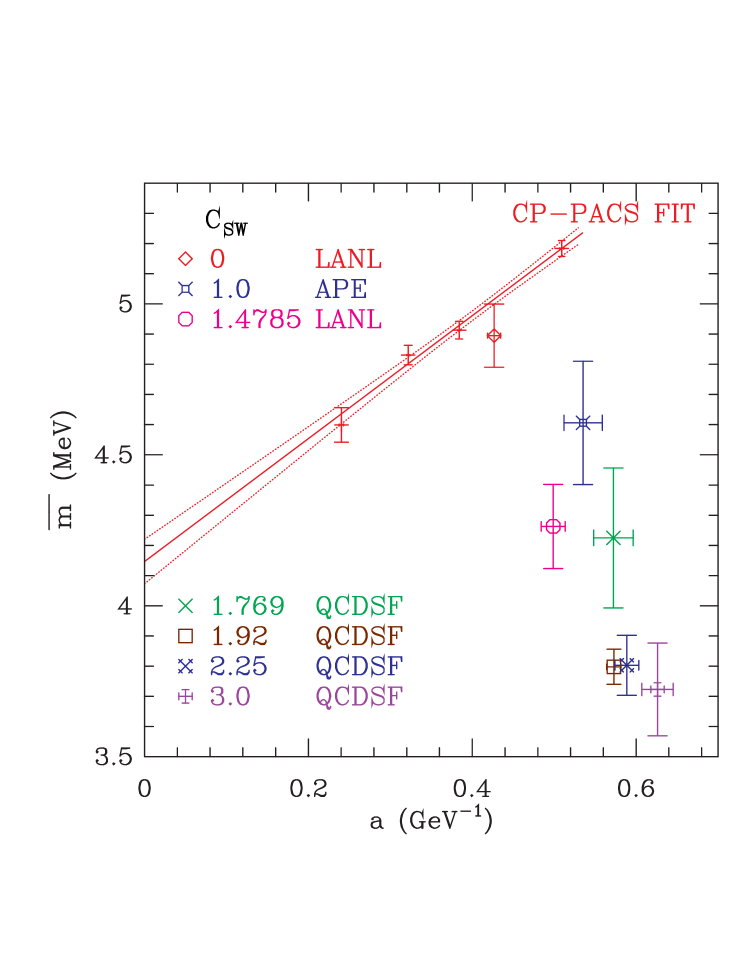
Figure 3: Behavior of $\overline{m}$ and $a(M_{\rho})$ as a function of the clover coefficient $C_{SW}$ at $\beta=6.0$. Also shown are the CP-PACS data and fit from Fig. 1.

The most extensive data are using the tadpole improved clover action (we do not distinguish between tree-level and 1-loop improved as the difference in $C_{SW}$ is small and we assume that it amounts to a negligible change in quark masses). These data for $\overline{m}$ from JLQCD [24, 25], LANL [26], and UKQCD [27] collaborations are shown in Fig. 4. We also show the Fermilab data given in [9]. Of the $\approx 10\%$ difference between JLQCD and Fermilab data at $\beta=5.9$ and $6.1$, $\approx 6\%$ comes from the setting of $a$ (Fermilab uses $1P-1S$ splitting in charmonium), and the rest from differences in $B_{\pi}$ and conversion to $\overline{\rm MS}$. Since the data needed for extracting $a(M_{\rho})$ for the Fermilab runs are not available, we cannot use these points in our continuum extrapolation. A fit to the rest of the data, assuming that the errors are $O(\alpha a)$, gives

$$\hbox{$\overline{m}$}=3.84(10){\rm MeV}[1+1.0{\rm GeV}\ \alpha(a)\ a],$$ (13)

shown by the fancy square at $a=0$. An analysis of $m_{s}(M_{K})$ and $m_{s}(M_{\phi})$ gives

$$m_{s}(M_{\phi})\mskip-3.0mu = \mskip-3.0mu117(8){\rm MeV}[1+1.5{\rm GeV}\alpha(a)a]$$

$$m_{s}(M_{K})\mskip-3.0mu = \mskip-3.0mu99(3){\rm MeV}[1+1.0{\rm GeV}\alpha(a)a].$$ (14)

In the figure we plot, for simplicity, the linear fit which has roughly the same $\chi^{2}$

$$\hbox{$\overline{m}$}=3.72(13){\rm MeV}[1+0.26{\rm GeV}\ a].$$ (15)

This lies $\approx 1\sigma$ below our preferred fit and value given in Eq. 13. Similar linear fits to the $m_{s}(M_{K})$ and $m_{s}(M_{\phi})$ data are shown in Fig. 5.

     

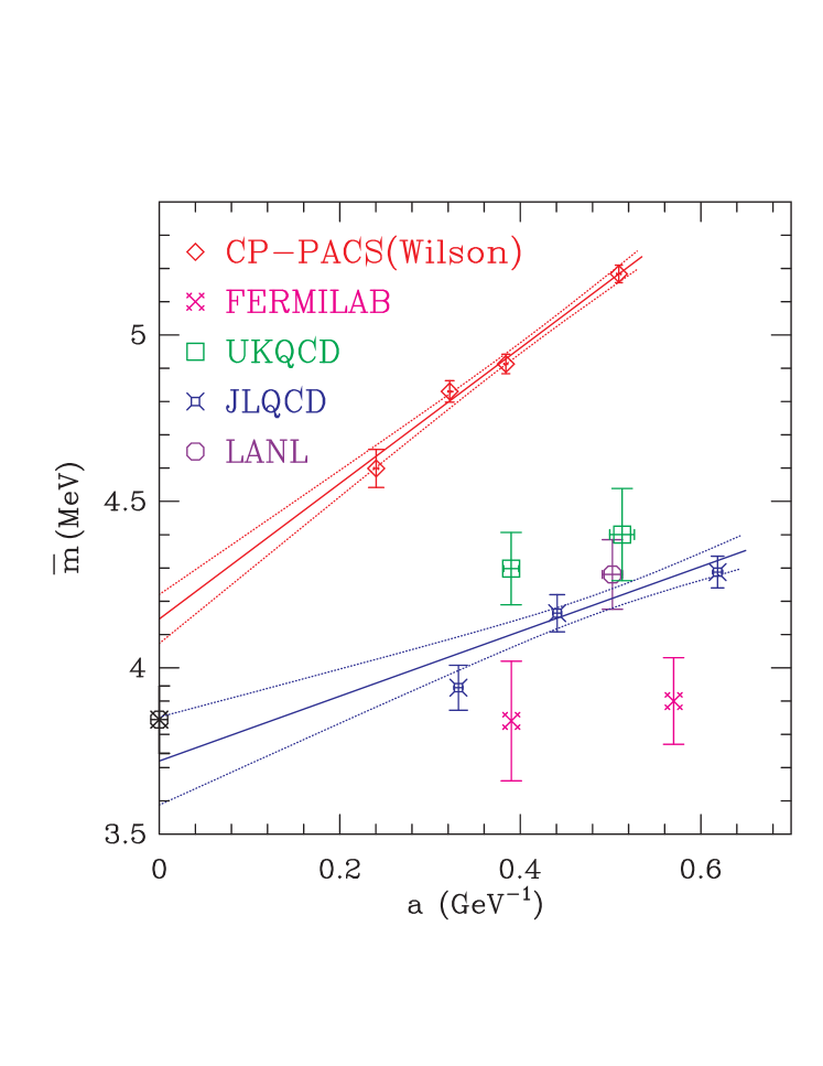
Figure 4: $\overline{m}$ from the TI clover data versus $a(M_{\rho})$. Also shown are CP-PACS Wilson data and fit from Fig. 1. Result of extrapolation in $\alpha a$ is shown by the fancy square at $a=0$.

     

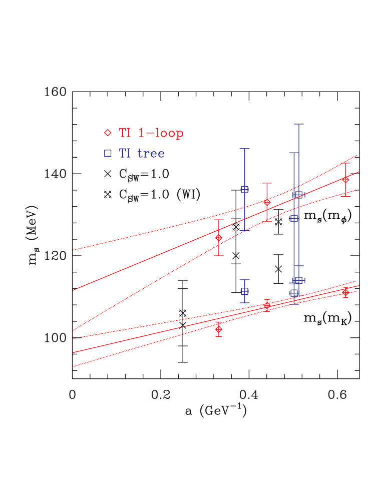
Figure 5: Data for $m_{s}(M_{K})$ and $m_{s}(M_{\phi})$ versus $a(M_{\rho})$ for TI clover fermions, along with simple linear extrapolation. Also shown are APE data with $C_{SW}=1$ for comparison.

The APETO [28], QCDSF [29] and UKQCD [27] collaborations have calculated quark masses using the non-perturbative value of $C_{SW}$ determined by the ALPHA collaboration. The data for $\overline{m}$ by QCDSF and UKQCD at $\beta=6.0$ and $6.2$ are shown in Fig. 6 and compared to tadpole improved clover. We find the following features. At $\beta=6.0$, data with the WI (QCDSF) and HS (larger volume QCDSF and UKQCD) methods agree, and roughly lie on the tadpole improved clover line. Going to $\beta=6.2$, the QCDSF WI data show a small increase. Consequently, a fit to the two QCDSF-WI points, assuming $O(a^{2})$ errors, gives the large value $\hbox{$\overline{m}$}=5.1(2)$ MeV (the value in the Fig. 6 is slightly different as it is from our analysis). On the other hand the QCDSF-HS value decreases slightly, while the UKQCD-HS data (still preliminary) show no $a$ dependence. Our overall conclusion is that the range in $\beta$ is too narrow to allow a meaningful extrapolation in $a$ with just two points.

     

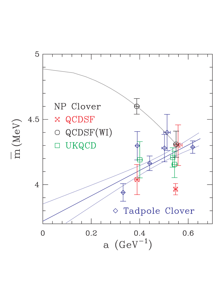
Figure 6: $\overline{m}$ from non-perturbative SW fermions. TI clover fit from Fig. 4 is also shown.

Both APETO [28] and QCDSF [29] have extracted $m_{s}$ at $\beta=6.2$ on $24^{3}\times 48$ lattices. Their raw data for pseudoscalar and vector masses are consistent. Since the extraction of $m_{s}$ includes $ma$ corrections to the renormalization constants, their results are correct to $O(a)$. The estimates of $m_{s}$ are $111(15)$ and $102(2)$ MeV respectively. QCDSF find a small increase between $\beta=6.0$ and $\beta=6.2$, and their value extrapolated to $a=0$ is $112(5)$ MeV. Higher statistics and larger lattices data at other values of $\beta$ are expected in the next year. These will improve the reliability of the extrapolation to the continuum limit.

4.2 Staggered Fermions

The advantage of staggered fermion formulation is the remnant chiral symmetry that guarantees Ward identities as in the continuum. As a result $Z_{A}=1$ and $Z_{S}=Z_{P}$, and the quark mass is only multiplicatively renormalized. Consequently, the two methods for determining quark masses, HS and WI, are the same. The sticky point is that the finite piece in TI 1-loop expression $Z_{m}=1/Z_{P}^{local}=1-\frac{\alpha_{s}}{4\pi}(8\log(\mu a)-39.1)$ is very large. Therefore, the 1-loop matching between lattice and continuum may not be reliable. Second, the 1996 data at $\beta>6.3$ was preliminary and suggested a small increase with $\beta$. There has been progress on both fronts in the last year. First, a partially non-perturbative analysis of the reliability of $Z_{P}$ has been done by Gupta, Kilcup, and Sharpe [30], and secondly there is new data by the JLQCD [31] and MILC [32] collaborations.

The basic idea of the partially non-perturbative analysis is that if $Z_{P}^{local}$ is large, then one could get a more reliable estimate using

$$Z_{P}^{local}=Z_{P}^{smeared}\times\left({Z_{P}^{local}\over Z_{P}^{smeared}}\right)$$ (16)

where “smeared” is any discretization of the pseudoscalar density that has a reliable perturbative expansion. The ratio in the parenthesis, which is a large factor, is calculated non-perturbatively. On the basis of such an analysis, Gupta, Kilcup, and Sharpe found that the 1-loop perturbative expression for $Z_{P}^{local}$ is $\sim 5\%$ smaller than the partially non-perturbative result at $\beta=6.0$. The caveat in this calculation is that the non-perturbative determination of the ratio shows large $O(a^{2})$ discretization errors, and the extrapolation to $a=0$ is based on only two points at $\beta=6.0$ and $6.2$. Thus, the calculation of the ratio needs corroboration. For the moment we apply this shift when presenting final estimates in Section 5.

The staggered fermion world data are shown in Fig. 7. The new data by JLQCD and MILC collaborations are consistent with the old, and confirm the small rise at weaker couplings. Assuming that the partially non-perturbative analysis of $Z_{P}$ validates the 1-loop result, and thus the non-monotonic behavior, we fit the data including $a^{2}$ and $a^{4}$ corrections. (Note that the absence of $O(a)$ corrections implies that the fit approaches $a=0$ with zero slope.) The results, in ${\rm MeV}$, are

$$\overline{m} = \mskip-12.0mu3.35(7)\big{[}1{-(.7{\rm GeV}\,a)^{2}}{+(1{\rm GeV}\,a)^{4}}\big{]}$$

$$m_{s}(M_{\phi})\mskip-12.0mu = \mskip-12.0mu104(5)\big{[}1{-(1{\rm GeV}\,a)^{2}}{+(1{\rm GeV}\,a)^{4}}\big{]}.$$ (17)

The discretization corrections are small, and account for the non-monotonic behavior, however, to resolve this issue a fully non-perturbative calculation of $Z_{m}$ is needed. The net upshot is that the staggered results using 1-loop $Z_{m}$ are basically unchanged, and raised by $\sim 5\%$ by using the partially non-perturbative calculation of $Z_{m}$.

     

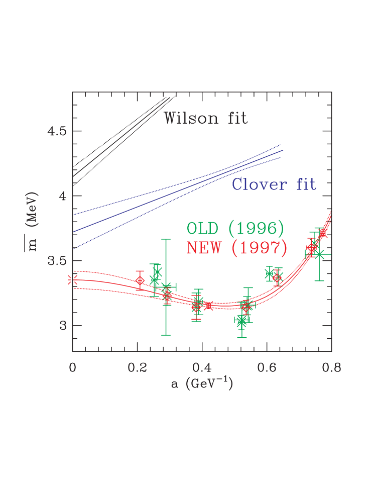
Figure 7: Staggered fermion data for $\overline{m}$ versus $a(m_{\rho})$. The fit assumes $a^{2}$ and $a^{4}$ corrections.

4.3 Non-perturbative $Z$’s: APE data

The APE collaboration has presented new data on the estimates of $\hbox{$\overline{m}$},m_{s}$, and $m_{c}$ using both the HS and WI methods [18]. They also provide a non-perturbative determination of $Z_{A},Z_{P}$ needed in the WI method, however, the $Z_{m}$ used in the HS method is still 1-loop. In their calculations of the NP $Z$’s for Wilson fermions bare operators are used, while for clover fermions a field rotation by $1+a{\hbox to0.0pt{\hbox to8.55695pt{\hfil/\hfil}\hss}\hbox{$D$}}/4$ is included.

The APE data are summarized in Table 1. We have also included a comparison of the tadpole improved $Z_{A}/Z_{P}$ with the non-perturbative factor $(1+\alpha_{s}C_{m}^{\rm Lan})Z_{A}/Z_{P}^{RI}$ with $\mu^{2}a^{2}=0.9648$. In keeping with the authors, who consider the $\beta=6.4$ lattices too small, we neglect the corresponding quark mass data. The first remarkable feature is that Wilson and clover fermions give consistent results for the WI method. Next, based on the consistency of the data at $\beta=6.0$ and $6.2$, the authors assume that there are no significant discretization errors. Thus, their final number $m_{s}(M_{K})=123\pm 4\pm 15$ is from the WI method, averaged over the Wilson and Clover fermions data at $\beta=6.0$ and $6.2$.

We consider the agreement between WI and the HS data fortuitous. If the difference between the perturbative and non-perturbative $Z_{m}$ is similar to that in $Z_{P}$, then the final HS results would be significantly different. Second, the CP-PACS/LANL data show a significant $a$ dependence which the APE data are not precise nor extensive enough to expose. This is the reason why their final value is higher than the world average given next.

Table 1: APE data for $m_{s}(M_{K})$ for Wilson (upper box) and $C_{SW}=1$ clover fermions. The perturbative and non-perturbative $Z$’s are also compared.

	$\beta=6.0$	$\beta=6.2$	$\beta=6.4$
$Z_{m}$( pert)	1.252	1.222	1.200
$Z_{A}/Z_{P}$( pert)	1.178	1.156	1.140
$Z_{A}/Z_{P}$(Npert)	1.659	1.507	1.345
$m_{s}$(WI) (MeV)	128(6)	117(8)	107(8)
$m_{s}$(HS) (MeV)	133(16)	130(16)	120(16)
$Z_{m}$( pert)	1.177	1.157	1.143
$Z_{A}/Z_{P}$( pert)	1.825	1.680	1.611
$Z_{A}/Z_{P}$(Npert)	2.350	2.033	1.700
$m_{s}$(WI) (MeV)	125(5)	127(9)	106(8)
$m_{s}$(HS) (MeV)	117(7)	120(9)	103(9)

5 Bottom line on quenched results

A summary of the quenched results, in ${\rm MeV}$, is

	Wilson	TI Clover	Staggered
$\overline{m}$	$4.1(1)$	$3.8(1)$	$3.5(1)$
$m_{s}(M_{K})$	$107(2)$	$99(3)$	$91(2)$
$m_{s}(M_{\phi})$	$139(11)$	$117(8)$	$109(5)$ .

These differences between Wilson, TI clover, and staggered results could easily be accounted for by the uncertainties in the extrapolations, and/or by the ratio of the non-perturbative to 1-loop estimates of $Z$’s. Thus, for our best estimate we take the mean and use the spread as the error. In case of $m_{s}$ we have an addition uncertainty coming from the dependence on the state used to extract it, $M_{K}$ versus $M_{K^{*}}$ (or equivalently $M_{\phi}$). This could be due to the quenched approximation or an artifact of having used linear chiral extrapolations. Since we do not have control over either of these two uncertainties, we again average over all the data. To these, we add a second uncertainty of $10\%$ as due to the determination of the scale $1/a$. Thus, our best estimates of $\overline{\rm MS}$ masses evaluated at $2$ GeV are

$$\overline{m} = 3.8(4)(4)\ {\rm MeV}$$

$$m_{s} = 110(20)(11)\ {\rm MeV}\,.$$ (18)

6 $N_{f}=2$ Wilson results

The SESAM collaboration has presented new data for $n_{f}=2$ Wilson fermions at $\beta=5.6$ [33]. The novel feature of their data is that pseudoscalar and vector masses have been calculated for degenerate ($\kappa^{V}=\kappa^{sea}$), and for non-degenerate ($\kappa^{V}\neq\kappa^{sea}$) combinations. The superscripts $V$ and ${sea}$ refer to valence and sea quarks respectively. Their data can be fit to

$$M_{\pi}^{2} = A_{\pi}+B_{\pi}^{V}\frac{1}{2\kappa^{V}}+B_{\pi}^{sea}\frac{1}{2\kappa^{sea}}$$

$$M_{\rho} = A_{\rho}+B_{\rho}^{V}\frac{1}{2\kappa^{V}}+B_{\rho}^{sea}\frac{1}{2\kappa^{sea}}\,.$$ (19)

As a result they study the dependence on both $\kappa^{V}$ and $\kappa^{sea}$ .

The first surprise of their calculation is a large dependence on $\kappa^{sea}$ ($B^{V}\sim B^{S}$). This is surprising because QCD perturbation theory and the success of lowest order $\chi$PT suggests that the dependence on sea quark masses should be small.

Their second important contribution is that they correctly point out that all previous extractions of $m_{s}$ from $n_{f}=2$ data are incorrect. Previous calculations were essentially calculating $m_{s}$ in a sea of strange quarks.

The last issue they raise is specific to Wilson-like fermions and concerns the zero of mass scale ($\kappa_{c}$), and concomitantly the definition of the quark mass. They discuss two possible ways of analyzing the data. (i) Degenerate extrapolation: determine $\kappa_{c}^{0}$ by extrapolating pion masses for the degenerate case $\kappa^{V}=\kappa^{sea}$ and measure all quark masses with respect to this $\kappa_{c}^{0}$. (ii) Partially quenched extrapolation: calculate $\overline{m}$, $m_{s}$ and $a$ for a fixed sea quark mass, and then extrapolate in the sea quark mass. They argue that the first method is the correct one and discard the second. It is at this point we disagree with them. What we now show is that if one uses the conventional perturbative $Z_{m}$ to relate the lattice mass to $\overline{\rm MS}$ scheme, then it is actually the partially quenched method that is more appropriate. We also argue that if $Z_{m}$ is calculated non-perturbatively, then both methods would give the same result for $\overline{m}$. Lastly, our analysis shows that the large dependence on $\kappa^{sea}$ is actually that of $\kappa_{c}$ on $\kappa^{sea}$, and not of physical masses.

The pole mass defined by the inverse propagator $S_{\psi}^{-1}=Z_{\psi}^{-1}({\hbox to0.0pt{\hbox to5.03125pt{\hfil/\hfil}\hss}\hbox{$p$}}-m)+\cdots$, can be written as

$$ma=\frac{1}{2\kappa^{V}}-8+\delta m\left(\alpha_{s},\frac{1}{2\kappa^{V}},\frac{1}{2\kappa^{sea}}\right)\,.$$ (20)

The linear divergence in $\delta m$ is absorbed in the definition of $\kappa_{c}^{0}$ (SESAM calls it $\kappa_{c}^{sea}$) as

$$\frac{1}{2\kappa_{c}^{0}}-8+\delta m\left(\alpha_{s},\frac{1}{2\kappa_{c}^{0}},\frac{1}{2\kappa_{c}^{0}}\right)=0\,.$$ (21)

Then, suppressing the dependence on $\alpha_{s}$,

$$ma = \frac{1}{2\kappa^{V}}-\frac{1}{2\kappa_{c}^{0}}+\delta m\left(\frac{1}{2\kappa^{V}},\frac{1}{2\kappa^{sea}}\right)$$ (22)

$$\hphantom{\frac{1}{2\kappa^{V}}-\frac{1}{2\kappa_{c}^{0}}}-\delta m\left(\frac{1}{2\kappa_{c}^{0}},\frac{1}{2\kappa_{c}^{0}}\right)\,.$$

Near $a=0$, $\kappa^{V}$ and $\kappa^{sea}$ approach $\kappa_{c}^{0}$, $i.e.$ the valence and the sea quark masses measured in lattice units approach zero, so we expand $\delta m$ about $\kappa^{V}=\kappa^{sea}=\kappa_{c}^{0}$

$$ma = \left(\frac{1}{2\kappa^{V}}-\frac{1}{2\kappa_{c}^{0}}\right)+\zeta^{V}\left(\frac{1}{2\kappa^{V}}-\frac{1}{2\kappa_{c}^{0}}\right)$$ (23)

$$\qquad{}+\zeta^{sea}\left(\frac{1}{2\kappa^{sea}}-\frac{1}{2\kappa_{c}^{0}}\right)$$

$$\equiv Z_{m}^{lat}\left(\frac{1}{2\kappa^{V}}-\frac{1}{2\kappa_{c}}\right),$$

where

$$Z_{m}^{lat} = 1+\zeta^{V}$$

$$\frac{1}{2\kappa_{c}} = \frac{1}{2\kappa_{c}^{0}}-\frac{\zeta^{sea}}{1+\zeta^{V}}\left(\frac{1}{2\kappa^{sea}}-\frac{1}{2\kappa_{c}^{0}}\right).$$ (24)

Note that both $Z_{m}^{lat}$ and $\kappa_{c}$ are the partially quenched ones. What has happened is that, for Wilson like fermions, along with the linear divergence which is absorbed in $1/2\kappa_{c}^{0}$, there is a finite piece of $O(1)$ that shifts the quark mass. As this finite piece is of $O(\hbox{$\overline{m}$})$ after extrapolation to the physical sea quark masses, its effect on the determination of $\overline{m}$ is dramatic, while it is a small correction in $m_{s}$.

In the degenerate case Eq. 23 becomes

$$ma = (1+\zeta^{V}+\zeta^{sea})\left(\frac{1}{2\kappa}-\frac{1}{2\kappa_{c}^{0}}\right)$$ (25)

$$= Z_{m}^{deg}\left(\frac{1}{2\kappa}-\frac{1}{2\kappa_{c}^{0}}\right),$$

where $Z_{m}^{deg}\equiv 1+\zeta^{V}+\zeta^{sea}$ has a contribution from valence and sea quarks. At 1-loop, $\zeta^{sea}=0$, therefore $Z_{m}^{lat}=Z_{m}^{deg}$ and $\kappa_{c}=\kappa_{c}^{0}$. What the SESAM data are telling us is that corrections to this 1-loop result are large, $i.e.$ $\zeta^{sea}\sim 1$. Thus, we arrive at the conclusion that combining the 1-loop $Z_{m}^{lat}$, which is independent of $\zeta^{sea}$, with the partially quenched extrapolation, which already incorporates $\zeta^{sea}$ as shown in Eq. 23, is more appropriate. Another way of saying this is that had $Z_{m}^{deg}$ been calculated non-perturbatively, one would have found $Z_{m}^{deg}\sim 2Z_{m}^{lat}$, which would have compensated for the smaller $\overline{m}$ obtained from the degenerate extrapolation.

SESAM, by measuring quark masses with respect to $\kappa_{c}^{0}$, extract $\hbox{$\overline{m}$}=2.7(2)$ MeV and $m_{s}=140(20)$. The large shift in $m_{s}/\hbox{$\overline{m}$}$ from $\chi$PT values is attributed to the effect of sea quarks, which could change as $a\to 0$. Our proposal for using the partially quenched extrapolation gives $\hbox{$\overline{m}$}=4.7(1)$ MeV which is $\sim 10\%$ below the quenched value at the same scale $a$ and roughly preserves the $\chi$PT ratio. Note, however, when using the partially quenched method there exist enhanced chiral logs, similar to those in the quenched approximation [34]. These afflict the theory at small quark masses, but for present masses this effect is expected to be negligible.

If the meson masses are completely independent of $\kappa^{sea}$, then

$${B_{\pi}^{sea}}/{B_{\pi}^{V}}={B_{\rho}^{sea}}/{B_{\rho}^{V}}\,.$$ (26)

The SESAM data bears this out within errors. However, when this constraint is used in the fits for the vector masses, they find high $\chi^{2}$s of about 50 for 25 degrees of freedom. We take this statistically significant, but small, effect to indicate that higher order terms in the chiral expansion do bring in small dependence of the meson masses on the sea quark mass.

In view of the above discussion, the only $n_{f}=2$ numbers that survive the above discussed ambiguity from the 1996 analysis are for staggered fermions, $\hbox{$\overline{m}$}\sim 2.7$ MeV. More data are necessary to establish the continuum limit in that case. For Wilson like fermions the final word on the values of $\overline{m}$ and $m_{s}$ has to await data using the WI method along with a non-perturbative determination of the $Z$’s.

7 Sum rule determinations of $\overline{m}$ and $m_{s}$

Progress in the sum-rules determination of quark masses has been incremental as has been the case for LQCD. Over time the perturbation expansion for the 2-point hadronic correction functions has been carried out to higher order, along with a better determination of $\Lambda_{QCD}^{(3)}$. Models for the hadronic spectral functions have been improved. The main limitation continues to be the lack of experimental data, with the one exception of $\tau$ decays. Thus, one has to model the spectral function rather than measure it. This slow but steady progress was, as summarized in Table 2, reaching a consensus by 1996 at $\hbox{$\overline{m}$}(2{\rm GeV})\approx 5{\rm MeV}$ and $m_{s}(2{\rm GeV})\approx 140{\rm MeV}$.

Sum rule calculations proceed in one of two ways. (i) Using axial or vector current Ward identities one writes a relation between two 2-point correlation functions, where the constant of proportionality are the quark masses [6, 7]. (ii) Evaluate a given correlation function both by saturating with known hadronic states and by evaluating it in perturbative QCD (PQCD) [36]. The PQCD expression depends on quark masses, and defines the scheme in which they are measured. Systematic errors arise from the (i) finite order calculation of PQCD expressions, (ii) the scale $\mu$ above which perturbative and hadronic solutions are valid and can be matched on the average (duality), and (iii) the ansatz for the hadronic spectral function.

Table 2: Values and bounds on $\overline{m}$ and $m_{s}$ from sumrules.

reference	$\overline{m}$ (MeV)	$m_{s}$ (MeV)
[37] 1989	${}=6.2(0.4)$	${}=138(8)$
[6] 1995	${}=4.7(1.0)$
[36] 1995	${}=5.1(0.7)$	${}=144(21)$
[7] 1995		${}=137(23)$
[38] 1996		${}=148(15)$
[39] 1997		${}=91-116$
[40] 1997		${}=115(22)$
[41] 1997	${}=4.9(1.9)$
[42] 1997	${}\geq 3.8-6$	${}\geq 118-189$
[43] 1997	${}\geq 3.4$	${}\geq 88(9)$
[44] 1997	${}\geq 4.1-4.4$	${}\geq 104-116$

In the last year, with the calculation of $\alpha_{s}^{3}$ terms in the perturbative expansions, the value of $\Lambda_{QCD}^{(3)}$ settling around $380{\rm MeV}$, and a critical reappraisal of the systematic errors in the sum-rule calculations [35], there has been a flurry of activity as shown in Table 2. The highlights of the new works are as follows.

The calculation of $O(\alpha_{s}^{3})$ terms and a detailed analysis of the convergence of the perturbation expansion suggests that the associated error is under control at $\approx 10\%$ level for $\mu\geq 2$ GeV [38].

Colangelo et al. [39] have extended the analysis of $m_{s}$ in [7, 38] by constructing the hadronic spectral function from known phase shift data. Similarly, Jamin [40] has also used a different parametrization of the hadronic spectral function using this phase shift data. In both cases the reanalysis lowers the estimate of the strange quark mass significantly as shown in Table 2.

Prades [41] has repeated the analysis of $\overline{m}$ incorporating the $\alpha_{s}^{3}$ corrections and using $\Lambda_{QCD}^{(3)}=380$ MeV. He reports a slightly higher value than in [6]. This is because Prades chooses the duality point at $\mu^{2}=2{\rm GeV}^{2}$, where $\overline{m}$ has a maximum. There is a significant decrease with $\mu$, the number dropping to $4.3(1.7)$ at $\mu^{2}=3{\rm GeV}^{2}$, and $3.8(1.5)$ at $\mu^{2}=4{\rm GeV}^{2}$. The rationale for the low choice of $\mu$ is that contributions not included in the spectral function will bolster the answer for larger $\mu$. This assumption needs to be substantiated.

Finally, a number of calculations have used the positivity of the spectral function to derive lower bounds [35, 42, 43, 44] which depend on $\mu$. Of these, the most stringent were reported by Lellouch at this conference [44, 45]. These bounds rule out the 1996 $n_{f}=2$ lattice results for $\mu\mathrel{\raise 2.0pt\hbox to8.0pt{\raise-5.0pt\hbox{$\sim$}\hss{$<$}}}2.8$ GeV. The hard to resolve question is – what is the scale $\mu$ at which PQCD, and thus the bound, becomes reliable? Unfortunately, this question cannot be answered at present.

8 Bottom quark mass

There are two determinations of $m_{b}$. The NRQCD collaboration [46] determine it from the Upsilon binding energy and the APE collaboration [47] use HQET. The two results agree:

$$m_{b}^{\overline{\rm MS}}(m_{b}^{\overline{\rm MS}}) = 4.15(5)(20)\ {\rm GeV}\quad{\rm(APE)}$$ (27)

$$= 4.16(15)\ {\rm GeV}\quad{\rm(NRQCD)}$$

The nice features of the NRQCD method are (i) determination of the scale from the spin averaged $1P-1S$ splitting. Data show that these splittings are independent of the precise tuning of the input mass $m^{0}_{H}$, and of the light quark action. (ii) tuning of $m^{0}_{H}$ using the kinetic mass

$$M=\lim_{p\to 0}\left({\partial^{2}E}/{\partial p^{2}}\right)^{-1}.$$ (28)

The heavy quark mass is then defined in two ways

$$m_{H}^{pole} = \frac{1}{2}[m_{H\overline{H}}-(E_{sim}-2E_{0})]$$

$$m_{H}^{\overline{\rm MS}} = Z^{pole\to\overline{\rm MS}}m_{H}^{pole}$$

$$m_{H}^{\overline{\rm MS}} = Z_{m}m_{H}^{0}\,.$$ (29)

The drawbacks are that $Z^{pole\to\overline{\rm MS}}$, $Z_{m}$, and $E_{0}$ (the energy of a zero-momentum quark state) are only known in PQCD to 1-loop. The two methods give consistent results, however, it is essential that the calculation be done at other values of $\beta$, to test for stability under variations of $a$.

The APE collaboration uses HQET to define

$$m_{b}(m_{b})=\left(M_{B}{-{\cal E}}+{\alpha_{s}(a)X\over a}\right)\left(1-{\alpha_{s}(m_{b})\over\pi}\right).$$

They explain how the linear divergence in the energy measured on the lattice, ${\cal E}$, is cancelled by that in the perturbative series whose first term is $\alpha_{s}(a)X/a$. The residual renormalon ambiguity is cancelled by a similar one in the second factor that relates the pole mass to the $\overline{\rm MS}$ mass. However, to take into account effects of higher orders in perturbation theory, they assign a systematic error of $200{\rm MeV}$ to the final result. We believe that their analysis of the cancellation of the renormalon ambiguity also applies to the NRQCD analysis, and with a similar residual uncertainty. The last issue concerning APE data is the stability under variations of the lattice spacing. We feel that by averaging over data at $\beta=6.0-6.4$, which shows a marginally significant variation, the APE collaboration may have missed an equally important source of uncertainty.

9 Charm quark mass

There are two new determinations of the charm quark mass by the APE [18] and the Fermilab collaborations [48]. The extraction by APE uses the same method as in [17]. The new features are that they use both the WI and the HS methods and use non-perturbative estimates of $Z$’s in the WI method. The drawback once again is that they average the data at $\beta=6.0,6.2$, and are not able to resolve discretization errors.

The Fermilab collaboration uses a combination of the NRQCD and Fermilab approaches. In their TI clover results, they include $O(ma)$ corrections in the determination of 1-loop $Z$’s, and calculate the $q^{*}$ in the matching factor using the Brodsky-Lepage-Mackenzie prescription, which they argue gets rid off possible infrared scales seen in the connection to pole mass. They find agreement in the extrapolated value between the two ways of calculating $m_{c}$, and also argue that quenching errors are expected to be small, unlike in the case of light quarks.

The final results are

$$m_{c}^{\overline{\rm MS}}(m_{c}^{\overline{\rm MS}}) = 1.525(40)(125){\rm GeV}\quad{\rm APE}\ .$$

$$m_{c}^{\overline{\rm MS}}(m_{c}^{\overline{\rm MS}}) = 1.33(8){\rm GeV}\qquad{\rm Fermilab}\ .$$ (30)

We do not consider the difference significant as it could easily be due to the different ways of setting the scale and/or due to the discretization errors that the APE data does not resolve.

Finally, we would like to mention the work of Bochkarev and Forcrand [49]. They calculate $m_{c}$ by evaluating the correlation functions arising in QCD sum-rules on the lattice. Their estimate, in the quenched approximation, is

$$m_{c}^{\overline{\rm MS}}(m_{c}^{\overline{\rm MS}})=1.22(5){\rm GeV}\ .$$ (31)

The errors include effects of discretization and finite volume, and in fact are dominated by the scale uncertainty. Given that these results were obtained on relatively small lattices ($16^{3}\times 32$) and with low statistics (20 configurations), the quoted accuracy is impressive. This approach should be investigated further.

10 Conclusions and Acknowledgements

Reliable estimates of quark masses have two immediate phenomenological consequences. (i) Standard Model predictions of $\epsilon^{\prime}/\epsilon$ are very sensitive to $m_{s}+m_{d}$ [50], and (ii) they constrain Supersymmetric models [51]. It is therefore exciting to report that the range listed in the Particle Data Book [52] has been significantly reduced.

In the last year the quenched estimates have been significantly improved, mainly due to the factor of 100 better data by the CP-PACS collaboration. There has been progress by the APE and ALPHA collaborations in the non-perturbative determination of renormalization constants. The SESAM analysis has lead to a deeper understanding of how to extract quark masses from $N_{f}=2$ simulations, however, we are no further along in obtaining continuum limit estimates. Since the quenching errors are the least well understood, it is this issue that needs maximum attention.

There has been progress in understanding errors in heavy quark analysis by the APE, Fermilab, and NRQCD collaborations. We now have “first generation” estimates of $m_{c}$ and $m_{b}$.

An area that has seen no progress is the study of isospin breaking effects. Knowing whether $m_{u}=0$ is important since a zero value solves the strong CP problem. The exploratory quenched calculations by Duncan et al. [13], where an electromagnetic field was added to quantify isospin breaking, reported a non-zero value of $m_{u}$: $(m_{d}-m_{u})/m_{s}=0.0249(3)$ and $m_{u}/m_{d}=0.512(6)$. Unfortunately, quenched calculations cannot address this question. The subtle point is that quark masses calculated from low energy phenomenology (or LQCD calculations with chiral extrapolations based on truncated $\chi$PT expansions) include instanton induced finite renormalizations [53]. What one wants is $m_{u}$ defined at a high scale. LQCD can directly probe this, but only if simulations are done including very light dynamical fermions whereby the influence of instanton zero modes on the light quark propagation is properly included.

Finally, it is exciting to see the rivalry between the LQCD and sum-rules estimates of quark masses heating up. We feel that both sides have made big strides in understanding and addressing the various sources of systematic errors, and estimates of masses have been tightened.

We thank C. Allton, L. Giusti, S. Gottlieb, S. Hashimoto, H. Hoeber, R. Kenway, A. Kronfeld, M. Luscher, S. Ohta, K. Schilling, G. Schierholz, and T. Yoshie, for providing details of their data in advance. We also acknowledge informative conversations with L. Lellouch, M. Lüscher and S. Sharpe. We thank DOE and the ACL for support of our work.

References

- [1]
- [2] J. Gasser etal., .
- [3] H. Leutwyler, .
- [4] H. Leutwyler, hep-ph/9609467.
- [5] D. Kaplan etal., .
- [6] J. Bijnens etal., .
- [7] M. Jamin etal., .
- [8] R. Gupta, etal., .
- [9] B. Gough etal., .
- [10] A. Ukawa, .
- [11] R. Gupta, .
- [12] P. Mackenzie, .
- [13] Duncan etal., .
- [14] S. Gottlieb, .
- [15] T. Bhattacharya, etal. .
- [16] S. Sharpe, .
- [17] C.R. Allton etal., .
- [18] L. Giusti, hep-lat/9709004, & private comm.
- [19] Bochicchio etal., .
- [20] G. Martinelli etal., .
- [21] S. Capitani etal., hep-lat/9709125.
- [22] J.A.M. Vermaseren etal., hep-ph/9703284.
- [23] T. Yoshie, these proceedings.
- [24] S. Hashimoto, these proceedings.
- [25] Y. Kuramashi, these proceedings.
- [26] T. Bhattacharya, R. Gupta, in preparation.
- [27] P. Rowland, these proceedings.
- [28] A. Cucchieri etal., hep-lat/9711040.
- [29] M. Göckeler etal., hep-lat/9707021.
- [30] G. Kilcup etal., hep-lat/9707006.
- [31] S. Aoki etal., , and private communications.
- [32] C. Bernard, hep-lat/9707014; and S. Gottlieb, private communications.
- [33] N. Eicker etal., hep-lat/9704019.
- [34] S. Sharpe, hep-lat/9707018.
- [35] T. Bhattacharya etal., hep-ph/9703455.
- [36] S. Narison, .
- [37] S. Narison, .
- [38] K.G. Chetyrkin etal., hep-ph/9612394.
- [39] P. Colangelo etal., hep-ph/9704249.
- [40] M. Jamin, hep-ph/9709484.
- [41] J. Prades, hep-ph/9708395.
- [42] F.J. Ynduráin, hep-ph/9708300.
- [43] H.G. Dosch etal., hep-ph/9709215.
- [44] L. Lellouch etal., hep-ph/9707523.
- [45] L. Lellouch, hep-ph/9709405.
- [46] C. Davies etal., .
- [47] V. Giménez etal., .
- [48] A. Kronfeld, hep-lat/9710007.
- [49] A. Bochkarev, P. de Forcrand, ; .
- [50] A.J. Buras etal., .
- [51] T. Blazek, etal., hep-ph/9611217.
- [52] R.M. Barnett etal., .
- [53] T. Banks, etal., hep-ph/9403203.