1 Introduction and motivations

The statistical mechanics of random manifolds provides a possible framework for a non-perturbative construction of a quantum theory of gravity (there exist several excellent reviews, e.g. [1], [2]). In this construction the standard recipes of lattice field theory are adopted, with a notable extension: the lattice itself becomes a dynamical object instead of being an inert scaffold. For fixed topology, the summation over geometries involved in the partition function, approximating Feynman’s path integral, is best implemented using the method of dynamical triangulations. The successes of this approach are particularly spectacular in two dimensions. The results obtained with models exactly solvable in the continuum formalism have been reproduced. Furthermore, completely new results, hardly attainable with another approach, have been derived. As an example, let us quote the beautiful calculation of the ”two-point” invariant correlation function in Ref. [3]. The method of dynamical triangulations is also applicable to four dimensional gravity. However, and this is not a surprise, the construction of a viable theory is much more difficult in four than in two dimensions.

At $d=2$ the Einstein term in the action is a topological invariant and the dynamics is insensitive to the corresponding coupling constant, as long as the topology of the manifold is kept fixed. For $d>2$ one finds that changing the (lattice analogue) of the Newton constant can modify the intrinsic geometry of the manifold. A phase transition is observed, separating two phases: in one the manifolds are crumpled, in the other they are elongated and resemble branched polymers. The transition was first discovered at $d=3$, and is there of first order [4]. The latent heat is large, in agreement with the generic picture suggested by mean field arguments [5]. The transition found at $d=4$ was initially thought to be continuous [6], but a more recent study [7] has furnished the evidence that it is actually of first order too, but with a very small latent heat. This finding has been confirmed by further work [8]. The smallness of the latent heat remains, however, a mystery. On the other hand, the dynamics of the transition has been to a large extent elucidated [9, 10, 11].

In Ref. [12] it has been emphasized that the crumpled $\to$ elongated transition occurs in all dimensions, but at $d=2$ this happens only when the central charge $c$ of matter fields is large enough. By lowering $c$ below unity one enters the Liouville phase, where a sensible continuum limit can be defined. There exists a heuristic argument [13] explaining that: when, increasing $c$, one crosses the magic value $c=1$ there occurs a condensation of metric singularities (“spikes”) and a collapse of the Euclidean space-time. The continuum formalism and the known dynamics of the conformal factor (Liouville action) can be used to calculate the free energy of spikes. The authors of Ref. [12] have suggested that a similar phenomenon might occur at $d=4$. Using the effective action for the conformal factor calculated in Ref. [14], the free energy/spike is:

$$F=\left[{{1411+N_{S}+11N_{F}+62N_{V}-28}\over{360}}-4\right]\;\ln{{\rho}\over a}\;.$$ (1)

The logarithmic factor on the right-hand side can be made arbitrarily large by taking a sufficiently spiky spike. The symbols $N_{S,F,V}$ refer to the number of massless scalar, fermion and vector fields contributing to the trace anomaly. The number $1411$ comes from a one loop calculation of the contribution of transverse gravitons and $28$ from ghosts and from quantum fluctuations of the conformal factor itself. This suggests that in the absence of matter fields the theory has no sensible vacuum and that this instability is lifted when the number of matter fields is large enough. As emphasized in Ref. [14], it is remarkable that the sign of the contributions of matter and ghost fields is in 4d opposite to that found in 2d. Thus in 4d one stabilizes the theory by adding matter fields, while in 2d the contrary happens. This idea has been further expanded in Ref. [15].

In two dimensions the effective action behind the estimate of the contribution of spikes can be derived essentially rigorously. It should be emphasized that this is not the case in four dimensions, because it is not clear how to treat the transverse part of the metric. Nevertheless, we consider the conjecture discussed above sufficiently interesting to investigate the influence of matter on the geometry in 4d simplicial quantum gravity, although earlier investigations have not observed any non-trivial effects of the matter sector [16].

Since the right-hand side of Eq. (1) depends most strongly on the number of vector fields, we consider in this paper only continuous vector gauge fields, which have not been studied previously in 4d simplicial gravity. The model is defined in Section 2. In Section 3 we discuss the strong coupling expansion of the partition function for simplicial gravity interacting with any number of gauge vector fields. Our analysis of this series indicates that polymerization is suppressed when $N_{V}>2$. We check this point in Section 4, where the results of our Monte Carlo simulations are presented. Our speculations and conclusions form the content of Section 5.

2 The model

The action is a sum of two parts. The first is the Einstein-Hilbert action, which for a 4d simplicial manifold reads:

$$S_{G}\,=\,-\kappa_{2}N_{2}+\kappa_{4}N_{4}\;,$$ (2)

where $N_{k}$ denotes the number of $k$-simplexes. The second part is

$$S_{M}\,=\,\sum_{t_{abc}}o(t_{abc})\left[A(l_{ab})+A(l_{bc})+A(l_{ca})\right]^{2}\;,$$ (3)

where $A(l_{ab})$ is a $U(1)$ gauge field living on link $l_{ab}$ and $A(l_{ab})=-A(l_{ba})$. The sum extends over all triangles $t_{abc}$ of the random lattice and $o(t_{abc})$ denotes the order of the triangle $t_{abc}$, i.e. the number of simplexes sharing this triangle. Since we adopt a non-compact version of the theory, with a Gaussian action, there is no need to introduce a coupling in front of the sum on the right-hand side above.

We work in a pseudo-canonical ensemble of (spherical) manifolds, with almost fixed $N_{4}$. The model is defined by the partition function:

$$Z(\kappa_{2},\bar{N}_{4})\,=\,\sum_{T}W(T)\int^{\prime}\prod_{l\in T}dA(l)\;\;{\rm e}^{\textstyle-S_{G}-S_{M}-{\delta\over 2}(N_{4}-\bar{N}_{4})^{2}}.$$ (4)

The sum is over all distinct triangulations $T$ and $W(T)$ is the symmetry factor taking care of equivalent re-labelings of vertexes. The prime indicates that the zero modes of the gauge field are not integrated. As is well known, the volume conserving local move is not ergodic, hence we must allow the volume to fluctuate. The quadratic potential term added to the action ensures, for an appropriate choice of $\delta$, that these fluctuations are small. The parameter $\kappa_{4}$ is adjusted so that $N_{4}$ fluctuates around a mean volume $\bar{N}_{4}$.

The Monte Carlo algorithm is constructed following one of the standard recipes of grand-canonical simulations [17]. A geometry move is done in two steps: first one integrates out the changing matter degrees of freedom, then the move is accepted/rejected based on a Metropolis test. If it is accepted, new matter fields are generated from a heatbath distribution, if new links are created, or disregarded if links have been removed. A geometry sweep consists of $N_{4}$ attempted (randomly chosen) geometry moves. Matter fields are updated using heatbath and overrelaxation algorithms. In a heatbath update the field is generated from the Gaussian distribution appearing in the partition function. In an overrelaxation update the field is given its “image” value: $A(l)\to-A(l)+2\bar{A}$, where $\bar{A}$ is the average over neighboring fields. A heatbath, or overrelaxation, sweep consists of $N_{1}$ attempted updates. The relative frequency of geometry and matter sweeps is chosen so as to minimize both the auto-correlation time and the CPU demand; we use typically one heatbath sweep followed by one overrelaxation sweep, after each geometry sweep. Measurements are done when $N_{4}=\bar{N}_{4}$, and are separated by a constant number of “passes” through $N_{4}=\bar{N}_{4}$. This number is chosen so that the system makes approximately 10 geometry sweeps between two successive measures.

3 The strong coupling expansion

In parallel to the development of the Monte Carlo code, we have calculated successive terms of the strong coupling expansion of the partition function Eq. (4). This calculation is split into two distinct parts: First, for a given triangulation, one has to find the symmetry factor: $W(T)=1/(\mbox{\rm number of equivalent re-labelings of}\;T)\;$. Second, one has to calculate the determinant $\Delta$, resulting from the Gaussian integration over one species of gauge fields (with unobservable zero modes kept fixed).

We found the weights up to $N_{4}=18$ by inspection, in order to test our codes and to get some insight into the problem. For larger manifolds we used pure gravity Monte Carlo simulations to identify the distinct triangulations and to determine the corresponding symmetry factors numerically, counting the relative frequency of the triangulations. The symmetry factors are also calculated explicitly, by going through all permutations of vertex labelings; comparing this to the Monte Carlo results serves as a consistency check on the identification. Finally, the determinant $\Delta$ is calculated using Maple. We have pushed the calculation up to $N_{4}=30$; the different contributions to the partition function, Eq. (4), are shown in Table 1 for zero, one and three vector fields.

Table 1: The number of different graphs, $N_{g}$, for a fixed volume $N_{4}$ and fixed number of vertexes $N_{0}$, and the corresponding weights $W_{N_{V}}(N_{4},N_{0})$. This is shown both for pure gravity, and one and three vector fields coupled to gravity ($N_{V}=0$, 1, and 3). All weights are normalized with the value at $N_{4}=6$.

$N_{4}$	$N_{0}$	$N_{g}$	$W_{0}$	$W_{1}$	$W_{3}$
6	6	1	1	1	1
10	7	1	3	$0.097638467\ldots$	$1.03423\ldots\times 10^{-4}$
12	7	1	5	$0.030058406\ldots$	$1.08632\ldots\times 10^{-6}$
14	8	1	15	$0.018550484\ldots$	$2.83715\ldots\times 10^{-8}$
16	8	2	255/4	$0.015777808\ldots$	$9.68553\ldots\times 10^{-10}$
18	8	3	110	$0.005500465\ldots$	$1.38182\ldots\times 10^{-11}$
	9	3	95	$0.004759295\ldots$	$1.19996\ldots\times 10^{-11}$
20	8	2	225	$0.002512817\ldots$	$3.15034\ldots\times 10^{-13}$
	9	7	693	$0.007291315\ldots$	$8.14758\ldots\times 10^{-13}$
22	9	15	2460	$0.005728290\ldots$	$3.27573\ldots\times 10^{-14}$
	10	7	690	$0.001447804\ldots$	$6.46761\ldots\times 10^{-15}$
24	9	13	16365/2	$0.004226212\ldots$	$1.17586\ldots\times 10^{-15}$
	10	34	14625/2	$0.003378959\ldots$	$7.45244\ldots\times 10^{-16}$
26	9	50	17865	$0.001946262\ldots$	$2.34367\ldots\times 10^{-17}$
	10	124	39645	$0.003936950\ldots$	$3.97116\ldots\times 10^{-17}$
	11	30	5481	$0.000491334\ldots$	$4.06700\ldots\times 10^{-18}$
28	9	89	291555/7	$0.001058334\ldots$	$6.96159\ldots\times 10^{-19}$
	10	415	182820	$0.004119603\ldots$	$2.16619\ldots\times 10^{-18}$
	11	217	77057	$0.001534637\ldots$	$6.33995\ldots\times 10^{-19}$
30	9	139	73860	$0.000457581\ldots$	$1.78973\ldots\times 10^{-20}$
	10	1276	672821	$0.003427165\ldots$	$9.13722\ldots\times 10^{-20}$
	11	1208	564000	$0.002507268\ldots$	$5.17157\ldots\times 10^{-20}$
	12	143	46376	$0.000179907\ldots$	$2.84432\ldots\times 10^{-21}$

The big advantage of the strong coupling approach is that once the weights and the determinants have been calculated, it does not cost any effort to change $\kappa_{2}$ and/or the number of matter fields. The series has been analyzed using the ratio method to extract the string susceptibility exponent $\gamma$ (cf. Ref. [18]), assuming the asymptotic behavior of the partition function:

$$Z(\bar{N}_{4})\;\sim\;{\rm e}^{\textstyle\kappa_{4}^{c}\bar{N}_{4}}\;\bar{N}_{4}^{\gamma-3}.$$ (5)

Actually, only every second term of the series can be used for this purpose. One finds an oscillation in the behavior of the coefficients; a closer look reveals that the complete series is a sum of two. If one estimates the critical coupling using these series separately, the two estimates approach the correct value from below and from above, respectively. For $\gamma$ we obtained more reliable results using the terms corresponding to $N_{4}=6,10,14,\dots$

Our results can be summarized as follows:

• For fixed (large) $\kappa_{2}$ the susceptibility exponent $\gamma$ becomes negative when the number $N_{V}$ of vector fields increases.

• For fixed $N_{V}$ and varying $\kappa_{2}$, the exponent $\gamma$ has a characteristic behavior: it is large negative for small enough $\kappa_{2}$, while it tends to a constant value for large $\kappa_{2}$. This limiting value is ${1\over 2}$, as expected, for pure gravity, and becomes negative for $N_{V}>2$. For intermediate $\kappa_{2}$ the estimate of the exponent is highly unstable, which is presumably a reflection of the existence of a phase transition. This is illustrated in Fig. (1). For $\kappa_{2}>\kappa_{2}^{c}$, on the other hand, the results are very stable, both with respect to variations in $\kappa_{2}$ and number of terms included in the analysis.

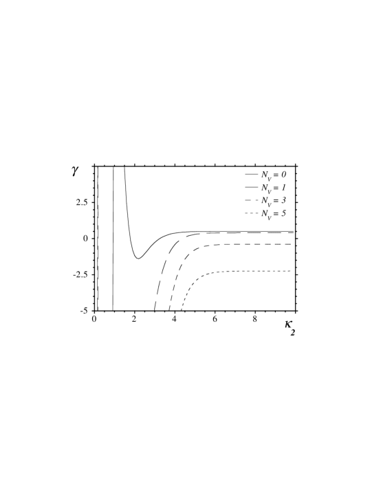
Figure 1: Variations of $\gamma$ with $\kappa_{2}$, for 0, 1, 3, and 5 vector fields coupled to gravity. These values are obtains using the ratio method to analyze the strong coupling series, including terms corresponding to $N_{4}=6$, 10, 14, 18, 22, 26, and 30.

These results suggest that for $N_{V}>2$ the branched polymer phase disappears, and is replaced by a new phase with a negative $\gamma$. This is similar to what happens in two dimensions, except in four dimensions $\gamma$ becomes more negative as the number of vector fields is increased. All this is in qualitative agreement with the expectations described in the Introduction. As these results have been obtained using relatively small triangulations, we have also carried out a series of Monte Carlo simulations to substantiate this picture; those results are presented in the next section.

4 Monte Carlo simulations

To understand better the phase structure of the model, as the number of vector fields $N_{V}$ is increased, we have performed Monte Carlo simulations using one and three vector fields, mostly on lattices with no more than 16K simplexes. As these are rather modest lattice volumes, we present our results with the appropriate reservations; it is well known that for pure gravity, simulations with such small volumes can give misleading informations, especially about the nature of the phase transition. We nevertheless believe that the results of our simulations, which agree well with the strong coupling expansion, present the correct qualitative picture.

As we want to compare our results to the corresponding simulations of pure gravity, we summarize what is observed in that case: There is a first-order transition [7, 8] separating a small $\kappa_{2}$ (strong coupling) crumpled phase from a large $\kappa_{2}$ (weak coupling) branched polymer phase; $\kappa_{2}^{c}\approx 1.29$. The crumpled phase is characterized by two singular vertexes, connected to an extensive fraction of the total volume, i.e. their local volume grows like $N_{4}$. Those vertexes are joined together by a sub-singular link; its local volume grows like $N_{4}^{2/3}$. This singular structure is not present in the branched polymer phase, it dissolves at the phase transition. In simulations on small lattices one actually observes that the transition occurs in two steps [10, 11, 19]; first the sub-singular link is dissolved, later, at weaker coupling, the singular vertexes disappear. Those two sub-transitions, however, seem to merge as the volume is increased.

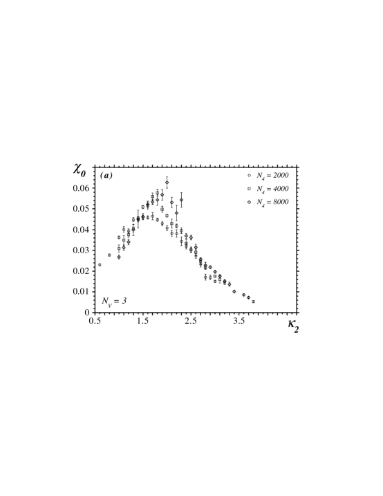
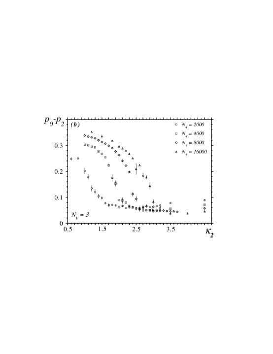
Figure 2: (a) The node susceptibility $\chi_{0}$, for three vector fields coupled to gravity, vs. $\kappa_{2}$. For $N_{4}=16000$ the statistics is not sufficient for a reliable estimate of $\chi_{0}$. (b) The corresponding change in the difference between the orders of the first and of the third most singular vertex, $p_{0}$ and $p_{2}$, normalized with the total volume $N_{4}$.

This picture does not change much if one adds one vector field to the model. We still observe two peaks in the node susceptibility, $\chi_{0}=(\left<N_{0}^{2}\right>-\left<N_{0}\right>^{2})/N_{4}$, presumably associated with the two sub-transitions discussed above. Those transition separate the usual crumpled and branched polymer phases. The second transition, at larger $\kappa_{2}$, is more pronounced, and for the largest volume (32K) we observe a clear signal of a first-order transition, i.e. fluctuations between two states in the timeseries of the energy. The corresponding latent heat appears to be smaller than in the case of pure gravity — maybe an indication that the transition becomes softer as matter is added.

A dramatic change occurs, however, when we introduce three vector fields to the model. We only observe a single peak in the node susceptibility, at $\kappa_{2}\approx 2$. Its height increases with the volume; see Fig. (2a). Presently, our data are not good enough to decide whether this is a real phase transition and, in the affirmative, what is the nature of the transition and the corresponding critical coupling. Simulations with higher statistics and at larger volumes are needed for that. We also observe a change in the geometry of the manifolds coinciding roughly with the peak in $\chi_{0}$: at strong couplings the system is in the crumpled phase, one has two well identified singular vertexes of almost the same order, separated by a large gap from the orders of other vertexes. As $\kappa_{2}$ increases the orders of these vertexes merge with the rest of the vertex order distribution. This is shown in Fig. (2b), where is plotted the difference between the orders of the first and the third most singular vertex: $p_{0}-p_{2}$. Combined, these results indicate that there still is a phase transition in this model.

Table 2: Measured values of the string susceptibility exponent $\gamma$ in the weak coupling (large $\kappa_{2}$) phase, for $N_{V}=3$.

$N_{4}$	$\kappa_{2}=4.5$	$\kappa_{2}=6.0$
2000	-0.22(2)
4000	-0.18(3)	-0.17(4)
8000	-0.23(3)
16000	-0.30(6)	-0.12(6)

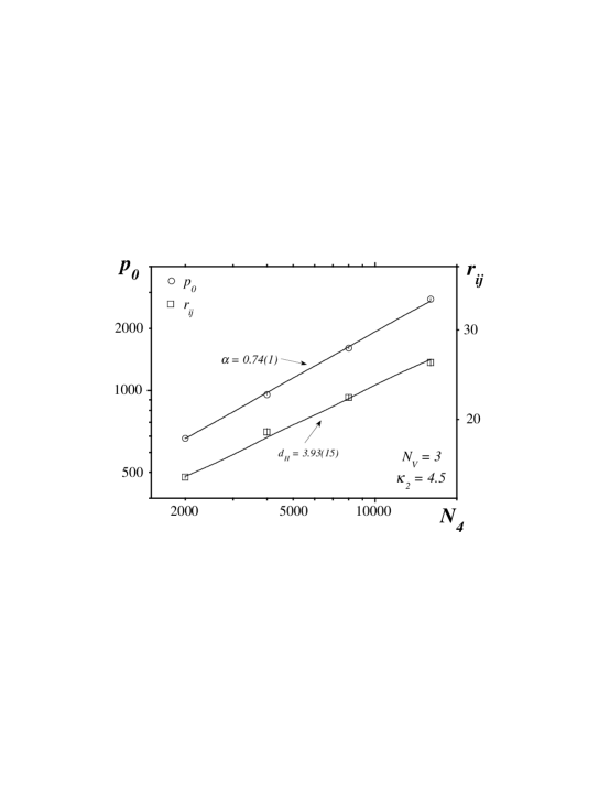
Figure 3: The scaling of both the largest vertex order, $p_{0}$, and of the average distance between two simplexes, $r_{ij}$, in the new weak coupling phase, for $N_{V}=3$ and at $\kappa_{2}=4.5$. The lines are the best linear fits to the data.

What about the respective phases? At small $\kappa_{2}$ there is the usual crumpled phase, but the weak coupling phase is no longer that of branched polymers. As mentioned above, it does not contain a singular vertex. This is best demonstrated by the scaling of the largest vertex order, which we show in Fig. (3) for $\kappa_{2}=4.5$. From the slope we see that the local volume grows like $N_{4}^{3/4}$, i.e. it is a vanishing fraction of the total volume. We have also measured the string susceptibility exponent $\gamma$ in this phase, extracted from the minbu distribution [20]. This we did for two values of $\kappa_{2}$ (4.5 and 6.0) and at different volumes (see Table 2). In all cases we get a consistent negative value, $\gamma\approx-0.2$, in reasonable agreement with the prediction from the strong coupling expansion, which is $\gamma\approx-0.38$. The fits to the minbu distributions are very good, which confirms the validity of the assumed asymptotic behavior Eq. (5). In contrast, it is not possible to extract any reliable value of $\gamma$ in the crumpled phase, nor close to the phase transition. Finally, we have measured the Hausdorff or fractal dimension $d_{H}$, using the scaling of the average distance between the simplexes [21]:

$$\left<r_{ij}\right>_{N_{4}}\;=\;\left<\sum_{r=0}^{\infty}r\;n(r)\right>\;\sim\;N_{4}^{1/d_{H}}\;,$$ (6)

were $n(r)$ counts the number of simplexes at a geodesic distance $r$ from a marked simplex. This is included in Fig. (3); a fit to Eq. (3) gives $d_{H}=3.97(15)$.

One apparent pathology of this new phase, is that the node number is very close to its upper kinematic bound, i.e. $\langle N_{0}\rangle/N_{4}\approx 0.25$. What this implies for the nature of the phase is not yet clear to us.

5 Summary and discussion

The most important result of this work is the discovery that by introducing matter fields one can prevent the standard collapse of 4d random manifolds into branched polymers. Contrary to all earlier investigations [16], we find a strong back-reaction of matter on geometry. This opens new research possibilities although, of course, one still faces many uncertainties and pathologies.

As already mentioned, the (discontinuous) phase transition observed with $N_{V}=1$ seems softer than that in pure gravity. Eq. (1) indicates that a weighted sum of $N_{S,F,V}$ controls the behavior of the theory; it is not excluded that, for some appropriate “combination” of matter fields, the transition might become continuous. This would be very exciting: one would have a relation between the matter content of the theory and its very existence.

The nature of the new weak coupling phase, which we have observed, for $N_{V}=3$, is also very intriguing. Our results suggest that this phase is characterized by a non-trivial negative $\gamma$ and that it has fractal dimension four, the same as the flat space. Yet it has some pathologies. Although its largest vertex order scales sub-linearly with the volume, it grows much faster than, for example, the largest vertex order in pure 2d gravity (where the growth is logarithmic). In addition, we observe that the number of nodes of the manifolds is very close to its kinematic bound. In spite of this, it is not excluded that a non-trivial continuum limit can be taken in this phase, i.e. that the whole phase is critical, as a negative susceptibility exponent would suggest. That would be analogous to what happens in two dimensions, but it is not clear what would be the nature of such a continuum theory, obtained without tuning the Newton’s constant to a critical value.

References

- [1] F. David, Simplicial Quantum Gravity and Random Lattices, Proc. Les Houches Summer School, Session LVII (1992).
- [2] J. Ambjørn, Quantization of Geometry, Proc. Les Houches Summer School, Session LXII (1994), (hep-th/9411179).
- [3] H. Kawai, N. Kawamoto, T. Mogami and Y. Watabiki, Phys. Lett. B306 (1993) 19; J. Ambjorn and Y. Watabiki, Nucl. Phys. B445 (1995) 129.
- [4] D.V. Boulatov and A. Krzywicki, Mod. Phys. Lett. A6 (1991) 3005; J. Ambjørn, D.V. Boulatov, A. Krzywicki and S. Varsted, Phys. Lett. B276 (1992) 432.
- [5] P. Bialas and Z. Burda, (hep-lat/9707028); P. Bialas, Z. Burda and D. Johnston, Nucl. Phys. B493 (1997) 505.
- [6] J. Ambjørn and J. Jurkiewicz, Phys. Lett. B278 (1992) 395; M. Agishtein and A.A. Migdal, Nucl. Phys. B385 (1992) 395; B. Brugmann and E. Marinari, Phys. Rev. Lett. 70 (1993)i 1908; S.M. Catterall, J.B. Kogut and R.L. Renken, Phys. Lett. B328 (1994) 277; B. de Bakker and J. Smit, Nucl. Phys. B439 (1995) 239; Z. Burda, J.P. Kownacki and A. Krzywicki, Phys. Lett. B356 (1995) 466.
- [7] P. Bialas, Z. Burda, A. Krzywicki and B. Petersson, Nucl. Phys. B472 (1996) 293.
- [8] B. de Bakker, Phys. Lett. B389 (1996) 238; S. Catterall, J. Kogut, R. Renken and G. Thorleifsson, Nucl. Phys. B53 (Proc. Suppl.) (1997) 756; S. Bilke, Z. Burda, A. Krzywicki and B. Petersson, Nucl. Phys. B53 (Proc. Suppl.) (1997) 743.
- [9] T. Hotta, T. Izubuchi and J. Nishimure, Prog. Theor. Phys. 94 (1995) 263; Nucl. Phys. B47 (Proc. Suppl.) (1996) 609; S.M. Catterall, R.L. Renken, J.B. Kogut and G. Thorleifsson, B468 (1996) 263;
- [10] P. Bialas, Z. Burda, B. Petersson and J. Tabaczek, Nucl. Phys. B495 (1997) 463.
- [11] S.M. Catterall, R.L. Renken and J.B. Kogut, (hep-lat/9709007).
- [12] J. Jurkiewicz and A. Krzywicki, Phys. Lett. B392 (1997) 291.
- [13] M.E. Cates, Europhys. Lett. 8 (1988) 719; A. Krzywicki, Phys. Rev. D41 (1990) 3086; F. David, Nucl. Phys. B368 (1992) 671.
- [14] I. Antoniadis and E. Mottola, Phys. Rev. D45 (1992) 2013; I. Antoniadis, P.O. Mazur and E. Mottola, Nucl. Phys. B388 (1992) 627.
- [15] I. Antoniadis, P.O. Mazur and E. Mottola, Phys. Lett. B394 (1997) 49.
- [16] J. Ambjørn, Z. Burda, J. Jurkiewicz and C.F. Kristjansen, Phys. Lett. B297 (1992) 253; Phys. Rev. D48 (1993) 3695; J. Ambjørn, S. Bilke, Z. Burda, J. Jurkiewicz and B. Petersson, Mod. Phys. Lett. A9 (1994) 2527; S.M. Catterall, J.B. Kogut and R.L. Renken, Nucl. Phys. B389 (1993) 601; Nucl. Phys. B422 (1994) 677.
- [17] J. Jurkiewicz, A. Krzywicki and B. Petersson, Phys. Lett. B177 (1986) 89.
- [18] F. David, J. Jurkiewicz, A. Krzywicki and B. Petersson, Nucl. Phys. B290 (1987) 218.
- [19] J. Tabaczek, M.Sc. Thesis, University of Bielefeld 1997.
- [20] J. Ambjørn, S. Jain, J. Jurkiewicz and C.F. Kristjansen, Phys. Lett. B305 (1993) 208.
- [21] J. Ambjørn and J. Jurkiewicz, Nucl. Phys. B451 (1995) 643.