Correlation functions and critical behaviour on fluctuating geometries

Abstract

We study the two–point correlation function in the model of branched polymers and its relation to the critical behaviour of the model. We show that the correlation function has a universal scaling form in the generic phase with the only scale given by the size of the polymer. We show that the origin of the singularity of the free energy at the critical point is different from that in the standard statistical models. The transition is related to the change of the dimensionality of the system.

, ,

The notion of correlation length is of a paramount importance in discrete field theoretical models. To define the continuum limit one requires correlation length to be infinite. This can be achieved by tuning the system to the continuous phase transition.

Consider as an example a spin system. The correlation length can be defined by the behaviour of the connected correlation function :

$$G_{c}(r,N)=\Big{\langle}\frac{1}{N}\sum_{i,j}^{N}\delta_{|i-j|,r}(s_{i}-\langle s\rangle_{N})(s_{j}-\langle s\rangle_{N})\Big{\rangle}_{N}$$ (1)

where the averaging goes over spin configurations on the lattice of size $N$. The delta function selects pairs at a distance $r$. This function has a well defined thermodynamic (large $N$) limit. In this limit near the transition point $G_{c}(r)$ behaves as

$$G_{c}(r)\sim\frac{1}{r^{\eta-1}}u\Big{(}\frac{r}{\xi}\Big{)}$$ (2)

where $\xi=\xi(\beta)$ is the correlation length which depends on a relevant coupling constant $\beta$ and $u(x)$ is a quickly decreasing universal function, typically an exponential. In the standard theory of continuous phase transitions the behaviour of $\xi$ near the critical point is characterised by the scaling exponent $\nu$:

$$\xi(\beta)\sim|\Delta\beta|^{-\nu}$$ (3)

where $\Delta\beta=\beta-\beta_{c}$ is the deviation from the critical value $\beta_{c}$. Integrating the connected correlation function (1) over $r$ one obtains magnetic susceptibility :

$$\sum_{r}G_{c}(r)=\frac{\langle M^{2}\rangle-\langle M\rangle^{2}}{N}\equiv\chi$$ (4)

where $M=\sum_{i}s_{i}$ is the total magnetization. The susceptibility is a second derivative of the free energy density $f(\beta,h)$ with respect to the magnetic field $h$ and has a singularity with a critical exponent $\gamma$ :

$$\chi(\beta)=\partial^{2}_{h}f(\beta,h)\sim|\Delta\beta|^{-\gamma}$$ (5)

Comparing with (2) one obtains

$$\chi\sim\xi^{-\eta+2}\sim|\Delta\beta|^{(\eta-2)\nu}$$ (6)

which leads to the Fisher scaling relation :

$$\gamma=(2-\eta)\nu$$ (7)

Similar reasoning can be applied to the energy–energy correlation function, which gives specific heat $c_{V}$ when integrated over $r$. In this case one obtains the scaling relation $\alpha=2-\nu d$ for the critical exponent of $c_{V}=\partial^{2}_{\beta}f\sim|\Delta\beta|^{-\alpha}$.

In other words the singularity of the free energy is directly related to the divergence of the correlation length. This picture is closely tied with the renormalization group analysis where infinite correlation length implies the scale invariance and hence the existence of a critical fixed point. At the critical point the free energy scales uniformly in relevant couplings and this yields singularity of the free energy.

In this paper we discuss a different source of the singularity of the free energy. We investigate a model with a random geometry. In such models the lattice is dynamical. There is an ensemble of lattices and one sums over all lattices in the ensemble. Geometry is defined by providing the distance definition between nodes.

The correlation function is defined in the same way as in the equation (1). Now the average is taken over the ensemble of lattices with size $N$, say with $N$ nodes. If there were fields on lattices one should additionally average over them, but here we consider the simplest model without the field dressing. One should note here that the correlation function in this case is not just a two-point function but rather a global correlator since the distance in the delta function depends on the whole geometry. Contrary to the quenched geometry models the delta function cannot be pulled outside the average brackets in (1).

In the following we consider the branched polymer model [1, 2, 3]. The partition function in this model is given as a weighted sum over an ensemble of trees. Trees are weighted by one-vertex branching weights. The partition function for the ensemble of trees with $N$ vertices is given by :

$$Z_{N}=\sum_{T\in{\mathcal{T}}_{N}}\frac{1}{C(T)}\exp\left(-\beta\sum_{i\in T}s(q_{i})\right)$$ (8)

where $q_{i}$ is order of vertex $i$ and $s$ is a one vertex action and $C(T)$ an appropriate symmetry factor of the graph. For some actions $s(q)$ the system has a phase transition. As an example we consider here the model with the action :

$$s(q)=\log(q)$$ (9)

The model has been solved in [2]. It has a fourth order phase transition at $\beta_{c}=2.47875...$. We discuss this particular form of the action to fix attention but the presented results concerning the universality and the critical behaviour hold also for a much broader class of actions where (9) is satisfied only asymptotically for large $q$ and which in particular allow for tuning the critical exponents and the order of the transition with the help of one effective parameter $\beta_{c}$ [3].

The second derivative of the free energy with respect to $\beta$ is finite but has a singularity :

$$f^{\prime\prime}\sim|\Delta\beta|^{\frac{3-\beta_{c}}{\beta_{c}-2}}$$ (10)

for small $\Delta\beta$. The model has two phases : the tree phase where the Hausdorff dimension is two and the bush phase where it is infinite. At the transition the Hausdorff dimension is $d_{H}=(\beta_{c}-1)/(\beta_{c}-2)$. The entropy exponent $\gamma_{s}$ changes from the generic value $1/2$ in the tree phase to $2-\beta_{c}$ in the bush phase and $\gamma_{s}=1/d_{H}$ at the transition [3].

The tree phase has highly universal properties. The volume–volume correlation function :

$$V(r,N)=\Big{\langle}\frac{1}{N}\sum_{i,j}^{N}\delta_{|i-j|,r}\Big{\rangle}_{N}$$ (11)

is for large $N$ given by the scaling formula [4, 5]:

$$V(r,N)=\sqrt{N}a\,v(x)$$ (12)

where the universal function is

$$v(x)=2xe^{-x^{2}}$$ (13)

and the scaling argument

$$x=\frac{a(r+d)}{\sqrt{N}}$$ (14)

with $d$ a finite shift which can be neglected in the large $N$ limit. This form holds in the whole tree phase. The only dependence on the coupling is in the coefficient $a=a(\beta)$ which rescales the distance $r$. The average distance between points on the branched polymers is

$$\langle r\rangle_{N}=\frac{\sum_{r}V(r,N)r}{\sum_{r}V(r,N)}=\frac{\sqrt{N}}{a}$$ (15)

The meaning of the formulae (12) and (15) is that the Hausdorff dimension is two as long as $a$ is finite. At the critical point $a$ diverges and the formula (12) does not hold anymore. At this point the Hausdorff dimension changes.

The volume-volume correlation function (11) is not a measure of geometric fluctuations. It is called correlation function only by analogy. Its geometric meaning is the average number of points at a distance $r$ from a given point. In this way the function (11) defines the dimensionality of the system. On a quenched geometry the the scaling (12) and (15) would give the canonical dimension.

To speak about geometric fluctuations and correlations one should consider a connected correlation function of the type (1) for a geometrical local quantity. In the branched polymer a good candidate for such a local quantity is any function which depends on a vertex order. In particular one can consider correlations between $q_{i}$ or between $s(q_{i})$ [5, 6]. The latter is an analog of the energy–energy correlation function and integrated over $r$ gives the second derivative of the free energy with respect to $\beta$.

Using similar techniques as for $V(r)$ one can find the large $N$ limit of other correlators. We sketch the derivation in the appendix. In particular for the two point connected correlator of the vertex operator $s(q)=\log(q)$ we obtain :

$$G_{c}(r,N) = \Big{\langle}\frac{1}{N}\sum_{i,j}^{N}\delta_{|i-j|,r}(s(q_{i})-\langle s(q)\rangle_{N})(s(q_{j})-\langle s(q)\rangle_{N})\Big{\rangle}_{N}$$ (16)

$$\approx \frac{1}{\sqrt{N}}\langle s(q)\rangle_{\infty}^{2}\,\delta^{2}a\,\,g(x)\qquad\qquad r>0,$$

where the scaling variable $x$ is again given by (14). The value at $r=0$ is a $N$ independent constant which we denote by $c=G_{c}(0,N)$. The universal function $g$ has the form :

$$g(x)=v^{\prime\prime}(x)=4x\left(2x^{2}-3\right)\exp\left(-x^{2}\right)\,.$$ (17)

The coefficients $a,\delta$ and $c$ depend on $\beta$. Near the transition they behave as :

$$\begin{array}[]{rl}a&\sim|\Delta\beta|^{-\frac{3-\beta_{c}}{2(\beta_{c}-2)}}\\ \delta&\sim|\Delta\beta|^{\frac{3-\beta_{c}}{2(\beta_{c}-2)}}\\ \langle s(q)\rangle_{\infty}&\sim\mbox{const}+|\Delta\beta|^{\frac{1}{\beta-2}}\\ c&\sim\mbox{const}+|\Delta\beta|^{\frac{1}{\beta-2}}\end{array}$$ (18)

One should note here that similar correlation function defined in the grand–canonical ensemble vanishes identically for $r>0$. It is essential that the averages, in particular $\langle s(q)\rangle_{N}$ are taken in the ensemble with a fixed number of nodes $N$. The source of the long–range correlations lies in the fact that for fixed $N$ the orders of vertices $q_{i}$ satisfy the global constraint

$$\sum_{i=1}^{N}q_{i}=2(N-1)$$ (19)

The second derivative of the universal function $v^{\prime\prime}(x)$ in the formula (17) comes about as follows. One can split the correlation function (16) into three terms :

$$G_{c}(r,N) = \Big{\langle}\frac{1}{N}\sum_{ij}^{N}\delta_{|i-j|,r}(s(q_{i})s(q_{j})\Big{\rangle}_{N}$$

$$-\,2\langle s(q)\rangle_{N}\Big{\langle}\frac{1}{N}\sum_{i,j}^{N}\delta_{|i-j|,r}s(q_{i})\Big{\rangle}_{N}$$

$$+\,\langle s(q)\rangle_{N}^{2}\Big{\langle}\frac{1}{N}\sum_{i,j}^{N}\delta_{|i-j|,r}\Big{\rangle}_{N}$$

Each of them is calculated separately. For $r>0$ and large $N$ they correspond to three terms in the following sum :

$$G_{c}(r,N) \approx \langle s(q)\rangle_{\infty}^{2}\Big{\{}V\big{(}r+2\frac{\delta}{a}\big{)}-2V\big{(}r+\frac{\delta}{a}\big{)}+V\big{(}r\big{)}\Big{\}}$$

$$= \langle s(q)\rangle_{\infty}^{2}\sqrt{N}a\Big{\{}v\Big{(}x+2\frac{\delta}{\sqrt{N}}\Big{)}-2v\Big{(}x+\frac{\delta}{\sqrt{N}}\Big{)}+v(x)\Big{\}}$$

$$\approx \frac{1}{\sqrt{N}}\langle s(q)\rangle_{\infty}^{2}a\delta^{2}v^{\prime\prime}(x)$$

where we used the fact that

$$\langle s(q)\rangle_{N}=\langle s(q)\rangle_{\infty}+O({1\over N})$$ (22)

The interesting point which we would like to emphasize is that the dressing of the geodesic line by the operators $s(q)$ at the ends results only in the effective shift of the argument $r$. This finite shift $\delta$ gives a subleading contribution to each of the correlators in the sum (Correlation functions and critical behaviour on fluctuating geometries). However as the leading terms cancel out only those subleading terms contribute to the end result. As we show below, the singularity of the free energy is directly related to the singularity of $\delta$.

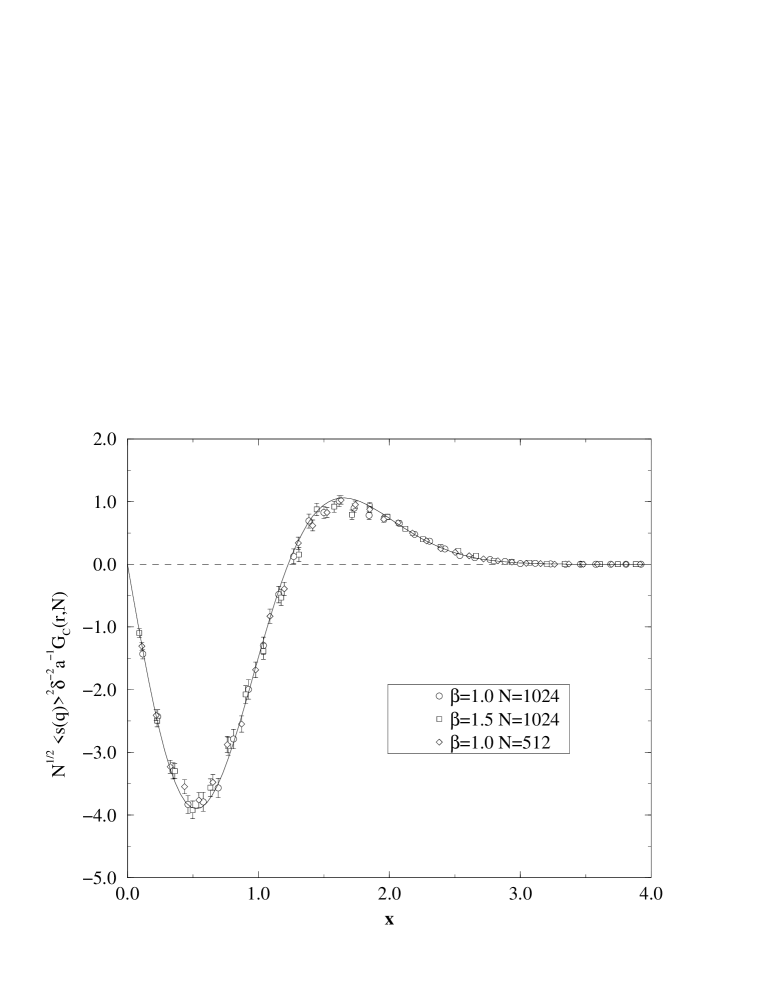
Figure 1: Scaling behaviour of the connected correlation function. The points are results of the direct computation of $G_{c}(r,N)$ by the Monte–Carlo program. For clarity only every third point is plotted. The line is the universal function $g(x)$. The argument $x=a(\beta)r/N^{1/2}$.

An important issue is the large $N$ limit. The formula (16) has been calculated for large $N$. In the scaling variable $x$ (14) the correlation function contains a part proportional to the delta function and the scaling part. The scaling part gives a non–vanishing contribution when the sum over $r>0$ is performed for $N\to\infty$ even though the contributions for individual $r$ vanish :

$$\sum_{r=1}^{\infty}G_{c}(r,N)\approx\int_{0}^{\infty}drG_{c}(r,N)\approx\langle s(q)\rangle_{\infty}^{2}\delta^{2}\int\mbox{d}xv^{\prime\prime}(x).$$ (23)

The second derivative of the free energy density becomes :

$$c_{V}=\partial^{2}_{\beta}f=\sum_{r=0}^{\infty}G_{c}(r,N)=c-2\delta^{2}\langle s(q)\rangle_{\infty}^{2}.$$ (24)

The first term $c$ comes from $N$ vertices and is a trivial self correlation. The second one is an anomalous term coming from correlations of pairs. The individual correlations vanish like $1/N$. The number of pairs, however, grows as $N^{2}$ so effectively the correlations contribute in the same order as $c$. This of course is possible only because the correlations are long range ie. they are not cut off by any finite scale. In fact it is the latter term which gives the singularity of the free energy density. From (18) we see that $a$ goes to infinity and $\delta$ to zero at the critical point. The singularity of $c$ is weaker than the one in $\delta^{2}$. Thus the singularity of the heat capacity $c_{V}$ comes from the coefficient $\delta^{2}$. Paradoxically the contribution from $\delta$ vanishes at the transition. The singularity arises from the way the coefficient $\delta$ vanishes and leads to the divergence of higher derivatives.

In the vicinity of the critical point the universal argument $x=ar/N^{1/2}$ has two large factors : $N^{1/2}$ and $a$ that diverge. One has to carefully define the limit $\Delta\beta\rightarrow 0$. If one did it naively and sent $\Delta\beta$ to zero at fixed $N$, the average distance $\langle r\rangle$ (15) would collapse to zero. In fact it does not. At the transition the Hausdorff dimension changes to $d_{H}=(\beta_{c}-1)/(\beta_{c}-2)$ [3] and the universal argument of the functions $v$ and $g$ changes to $x\propto r/N^{1/d_{H}}$. Also the function $v$ and $g$ themselves change the form. Just beyond the transition point the geometry collapses. The collapse results from the appearance of an additional mass term $e^{-m(\beta)r}$ in the correlation function with the non–zero mass independent on $N$. This mass fixes the average distance between points on the polymer to $1/m$ which is independent of $N$. The fact that the average distance (15) does not grow with the lattice size $N$ can be interpreted as an infinite Hausdorff dimension.

The model can be easily generalized to other actions. By a simple modification one has a possibility to tune $\beta_{c}$ in the range $(2,\infty)$[2]. For $2<\beta_{c}<3$ the critical behaviour of the coefficients $a,\delta$ and $c$ is still described by the same formulae (18). The coefficient $a$ diverges and $\delta$ gives the the singularity of the free energy. The situation changes for $\beta_{c}>3$ where both $a$, $\delta$ approach finite constants at the critical point. The singularities of both of them are of the form $\Delta\beta^{\beta_{c}-3}$. The singularity of $b$ is inherited by $c_{V}\sim\Delta\beta^{\beta_{c}-3}$. The fact that $a$ is finite at the transition means that the argument $x$ of the universal functions (12) and (17) preserves the form $x=ar/N^{1/2}$ and the Hausdorff dimension is two as in the tree phase. In the limiting case $\beta_{c}=3$ the system undergoes a strong third order phase transition with the singularity $f^{\prime\prime}\sim\log|\Delta\beta|^{-1}$.

Let us at the end briefly compare the critical behaviour of the model with the standard critical phenomena of statistical models. The general scaling Ansatz for a two-point correlation function involves two dimensionless ratios : $r/\xi$ and $r/N^{1/d_{H}}$. The singularity of the free energy arises when the correlation length $\xi$ diverges. In our model the scaling function involves only the argument $r/N^{1/d_{H}}$. In other worlds it has no other scale except the size of the system. One can say that the model is always critical ($\xi\to\infty$). The long–range correlations between orders of different vertices are not induced by local interactions but rather by the Euler relation (22). The mechanism of the transition is the same as in the balls-in-boxes model and relies on appearance of the surplus anomaly [7]. There the correlations between number of balls in two boxes vanish for large $N$ (this is in the analogy with the vanishing of $G_{c}(r,N)$ for fixed $r>0$ and $N\to\infty$), but this is compensated by the growing number of pairs of boxes over which we have to sum over. The anomaly corresponds to the singular vertex which changes the geometrical properties of the branched polymer and leads to the collapse which is associated with the appearance of the non scaling mass in the two point correlation function.

A similar phase transition between the branched polymer phase and the collapsed phase is observed in 4d simplicial gravity [10, 11, 12]. One can expect the same qualitative behaviour of the correlation function (1) for the curvature-curvature correlations in 4d simplicial gravity [13].

Two of the authors (P.B. & Z.B.) thank the Niels Bohr Institute for the hospitality during their stay, where the work was completed. The authors are grateful to J. Ambjørn for valuable comments and discussions. The work was partially financed by the KBN grants 2P03B04412 and 2P03B19609.

Appendix A

The correlation functions are constructed by means of the partition function of planted, rooted, planar trees. This partition function can be found from the following recursive equation [1]:

$$Z=e^{-\mu}F(Z)$$ (25)

where the generating function is

$$F(Z)=\sum_{q=1}e^{-\beta s(q)}Z^{q-1}\,.$$ (26)

For $\mu$ approaching a critical value $\mu_{C}$ from above, $Z$ has the following singularity :

$$Z(\mu)=Z_{0}(\beta)-Z_{1}(\beta)\sqrt{\Delta\mu}+\dots$$ (27)

The critical value $\mu_{C}$ corresponds in the large $N$ limit to the free–energy density of the canonical ensemble [2]. In particular

$$\langle s(q)\rangle_{N}=\partial_{\beta}f(\beta)=-\partial_{\beta}\mu_{C}(\beta)+O(\frac{1}{N})$$ (28)

As a function of $\beta$ the free energy $\mu_{C}$ has a singularity at a critical point $\beta_{C}$. This singularity appears also in the coefficients $Z_{i}$ of the expansion (27) [2, 5] :

$$1-Z_{0} \sim |\Delta\beta|^{\frac{1}{\beta_{C}-2}}$$ (29)

$$Z_{1} \sim |\Delta\beta|^{\frac{3-\beta_{C}}{2}}$$ (30)

The correlation functions in the grand–canonical ensemble can be calculated in terms of $Z(\mu,\beta)$ [4, 5] as :

$$\sum_{T\in\mathcal{T}}\sum_{i,j}\delta_{|i-j|,r} = \Big{(}1-\frac{Z}{\partial_{\mu}Z}\Big{)}^{r-1}Z^{2}$$ (31)

$$\sum_{T\in\mathcal{T}}\sum_{i,j}s(q_{i})\delta_{|i-j|,r} = \Big{(}1-\frac{Z}{\partial_{\mu}Z}\Big{)}^{r-1}Z^{2}\frac{\partial_{\beta}Z}{\partial_{\mu}Z}$$ (32)

$$\sum_{T\in\mathcal{T}}\sum_{i,j}s(q_{i})s(q_{j})\delta_{|i-j|,r} = \Big{(}1-\frac{Z}{\partial_{\mu}Z}\Big{)}^{r-1}\Big{(}\frac{\partial_{\beta}Z}{\partial_{\mu}Z}\Big{)}^{2}$$ (33)

which then can be transformed by Laplace transform to the canonical ensemble with a fixed size $N$ leading to the terms in (Correlation functions and critical behaviour on fluctuating geometries). The results (Correlation functions and critical behaviour on fluctuating geometries) correspond to the leading order terms of the Laplace transform calculated by the saddle point approximation.

References

- [1] J. Ambjørn, B. Durhuus, J. Fröhlich, P. Orland Nucl. Phys. B270 (1986) 457.
- [2] P. Bialas, Z. Burda Phys. Lett. B384 (1996) 75.
- [3] J. Jurkiewicz, A. Krzywicki Phys. Lett. B392 (1997) 291.
- [4] J. Ambjørn, B. Durhuus, T. Jónsson, Phys. Lett. B244
- [5] P. Bialas, Phys. Lett. B373 (1996) 289.
- [6] P. Bialas Nucl. Phys. B (Proc Suppl.) 53 (1997) 739.
- [7] P. Bialas, Z. Burda, D. Johnston Nucl. Phys. B493 (1997) 505.
- [8] P. Bialas, Z. Burda, A. Krzywicki, B. Petersson Nucl. Phys. B472 (1996) 293.
- [9] J. Ambjørn, J. Jurkiewicz, Nucl. Phys. B541 (1992) 643
- [10] P. Bialas, Z. Burda, B. Petersson, J. Tabaczek Nucl. Phys. B495 (1997) 463. (1990) 403.
- [11] P. Bialas, Z. Burda “Collapse of 4D random geometries” hep-lat/9707028
- [12] S. Catterall, R. Renken, J. Kogut “Singular Structure in 4D Simplicial Gravity” hep-lat/9709007
- [13] B .V. de Bakker, J. Smit Nucl. Phys. B454 (1995) 343.