Abstract

We consider the lattice regularization of $N=1$ supersymmetric Yang–Mills theory with Wilson fermions. This formulation breaks supersymmetry at any finite lattice spacing; we discuss how Ward identities can be used to define a supersymmetric continuum limit, which coincides with the point where the gluino becomes massless. As a first step towards the understanding of the zero gluino–mass limit, we present results on the quenched low-lying spectrum of SU(2) $N=1$ Super-Yang–Mills, at $\beta=2.6$ on a $V=16^{3}\times 32$ lattice, in the OZI approximation. Our results, in spite of the quenched and OZI approximations, are in remarkable agreement with theoretical predictions in the supersymmetric theory, for the states with masses which are not expected to get a large contribution from fermion loops.

Towards $N=1$ Super-Yang–Mills

on the Lattice

A. Donini^a, M. Guagnelli^b, P. Hernandez^b, A. Vladikas^c

^a Dip. di Fisica, Univ. di Roma “La Sapienza” and INFN, Sezione di Roma,

P.le A. Moro 2, I-00185 Roma, Italy.

^b Theory Division, CERN, 1211 Geneva 23, Switzerland.

^c INFN, Sezione di Roma II, and Dip. di Fisica, Univ. di Roma “Tor Vergata”,

Via della Ricerca Scientifica 1, I-00133 Roma, Italy.

CERN-TH/97-266

1 Introduction

Softly broken $N=1$ supersymmetry gives a natural solution to the long-standing hierarchy problem present in the Standard Model, considered as a low-energy effective model of a more fundamental theory that includes gravity. In recent years, many new results on the non-perturbative regime of supersymmetric gauge theories have been derived and/or conjectured [1]. However, the only proved results have been obtained in the context of extended supersymmetry ($N>1$), where the renormalization properties are severely constrained [2]. From these, rigorous results can also be derived in the phenomenologically more relevant cases of $N=1$ and $N=0$, through the introduction of explicit and perturbative soft-breaking terms [3]. Unfortunately, the analytical methods fail when the soft-breaking terms become large with respect to the scale of the strong dynamics. This is of course the most interesting regime, and the lattice is a good non-perturbative method to explore it.

In this work we will consider the case of $N=1$ Super-Yang–Mills theory (SYM). Some preliminary results for gauge observables in this theory have been presented in [4] and confirmed with a different method in [5]. The standard lore in SYM was conjectured a long time ago [6, 7] and our programme is to confirm this picture on the lattice. It is believed that these theories show confinement and a mass gap. Furthermore SUSY is expected to be unbroken. This expectation is based on the fact that the Witten index is not zero [8]. As will be explained in this work, SUSY Ward identities (WIs) can be used to study the issue of SUSY breaking on the lattice. At low energies, the relevant degrees of freedom are expected to be colourless composite fields of gluons and gluinos and the lowest-lying spectrum can be described by a low-energy effective supersymmetric Lagrangian [6]. The bound states belong to chiral supermultiplets. The lowest-lying chiral supermultiplet is expected to be [6]

$$\Phi=(\tilde{\pi},\tilde{\sigma},\tilde{\chi},F,G),$$ (1)

where $\tilde{\pi}=\bar{\lambda}\gamma_{5}\lambda$ is a pseudoscalar, $\tilde{\sigma}=\bar{\lambda}\lambda$ is a scalar, and $\tilde{\chi}=\frac{1}{2}\sigma_{\mu\nu}F_{\mu\nu}\lambda$ is a fermionic composite field (here $\lambda$ denotes the gluino field and $F_{\mu\nu}$ the gluon field tensor). The fields $F$ and $G$ (scalar and pseudoscalar respectively) are auxiliary fields with no dynamics. In the supersymmetric limit, these particles should be degenerate in mass [6]. With supersymmetry softly broken by a gluino mass term, the mass splittings between $\tilde{\pi},\tilde{\sigma}$ and $\tilde{\chi}$ have been computed, to lowest order in the gluino mass, in [9].

In this paper we will be concerned with supersymmetric $SU(2)$. Our lattice formulation, described in section 2, is simply the Wilson action for the bosonic components and the Wilson–Dirac operator for the gluinos. The presence of Majorana fermions implies a modification of the standard measure of the path integral and the rules of Wick contractions. This lattice regularization breaks supersymmetry for two reasons. Firstly the breaking of Lorentz symmetry implies that the supersymmetric algebra cannot be satisfied at finite lattice spacing. Secondly, the Wilson term induces a finite mass for the gluino which splits the supermultiplet. This problem is, however, not very different from the explicit breaking of chiral symmetry in lattice QCD with Wilson fermions and can be handled in the same way [10]. The essential point is that the symmetry-breaking effects that survive the continuum limit can be eliminated through renormalization (if there are no SUSY anomalies), which in this case amounts to a proper tuning of the gluino bare mass. This follows from very general principles. Since the lattice theory is asymptotically free, the continuum limit can be defined at the UV fixed point. In this limit the lattice theory must be equivalent to a theory with the same degrees of freedom and all possible interactions of dimension four or less, which are compatible with the symmetries of the lattice action. In particular, from the exact gauge and cubic symmetries of the lattice action, it follows that the only possible continuum action is the one corresponding to SYM, augmented by a gluino mass term. So even though SUSY is broken at finite lattice spacing in a very complicated way, the continuum limit of this theory is softly broken SYM, provided there are no supersymmetric anomalies. Through a non-perturbative tuning of the bare gluino mass, a supersymmetric limit can be obtained, which coincides with the zero gluino-mass limit [10]. In section 3, we review how this can be achieved in practice through the use of Ward identities. Moreover, we argue that an important simplification of this method consists in the implementation of the OZI approximation. A method to determine the order parameter of supersymmetry breaking using WI is also discussed in the same section.

The low-lying spectrum defined in (1) can be computed from exponential decay of the two-point correlation functions at large time separations, as described in section 4. The measurements in the scalar and pseudoscalar channels are completely analogous to their QCD counterparts. The fermionic composite $\tilde{\chi}$ is a new channel that presents difficulties, which closely resemble those encountered in glueball spectroscopy in QCD and, fortunately, can be overcome with the same type of techniques.

In sections 5 and 6, we present our spectroscopy results in the quenched and OZI approximations. Although SUSY is lost in these approximations, this is a convenient first step, which enables lattice calibrations and optimizations of the observables, without the high computer cost of dynamical fermion simulations. It is also useful in the understanding of the zero gluino-mass limit in a simpler setting, where the chiral anomaly is switched off. As in quenched QCD, PCAC is expected to govern the chiral restoration of the theory in the continuum limit. Our results strongly support these expectations. Whenever comparison with the results of [9] is possible, we find agreement within large statistical errors. A preliminary version of our results can be found in [11].

2 Lattice gauge theory with Majorana fermions

We use the lattice regularization of the $N=1$ SYM, first proposed in ref. [10]. The gauge field (the gluon), is the usual link variable $U_{\mu}(x)$ in the fundamental representation of the gauge group $SU(N_{c})$ (here $N_{c}=2$). The purely gluonic part of the action $S_{g}$ is the usual sum over plaquettes formed by link variables $U_{\mu}(x)$. The gluino $\lambda$ is in the adjoint representation of the gauge group and satisfies the Majorana condition

$$\lambda=\lambda^{{\cal C}}=C\bar{\lambda}^{T},\;\;\;\;\bar{\lambda}=\bar{\lambda}^{{\cal C}}=\lambda^{T}C,$$ (2)

where the superscript ${\cal C}$ stands for charge conjugation, the superscript $T$ for transposition in spin and colour indices (implicit in the above equations) and $C$ is the charge conjugation matrix. The fermionic action is the Wilson–Dirac operator for adjoint fermions, i.e.

$$S_{f}=\sum_{x,y}\bar{\lambda}^{a}_{\alpha}(x)\Delta^{ab}_{\alpha\beta}(x,y)\lambda^{b}_{\beta}(y)=\sum_{x,y}\lambda^{a}_{\alpha}(x)M^{ab}_{\alpha\beta}(x,y)\lambda^{b}_{\beta}(y),$$ (3)

where $M=C\Delta$ is the fermion matrix

$$M^{ab}_{\alpha\beta}(x,y) = \frac{1}{4}\sum_{\mu}V^{ab}_{\mu}(x)[C(\gamma_{\mu}-r)]_{\alpha\beta}\delta^{4}_{y,x+\hat{\mu}}$$ (4)

$$- \frac{1}{4}\sum_{\mu}V^{ab}_{\mu}(y)[C(\gamma_{\mu}+r)]_{\alpha\beta}\delta^{4}_{y,x-\hat{\mu}}$$

$$+ \frac{1}{2}(m_{0}+4r)\delta^{ab}C_{\alpha\beta}\delta^{4}_{y,x}.$$

The basic notation and index conventions are given in Appendix A. As usual, we have fixed $r=1$. The gauge field $V_{\mu}^{ab}(x)$ is defined by

$$V_{\mu}^{ab}(x)=2\;{\rm Tr}[U^{\dagger}_{\mu}(x)T^{a}U_{\mu}(x)T^{b}],$$ (5)

with the trace acting on colour indices in the fundamental representation. It satisfies the properties [4]

$$V_{\mu}^{ab}(x)=V_{\mu}^{ab}(x)^{\ast}=[V_{\mu}^{ab}(x)^{T}]^{-1},$$ (6)

where the transposition and inversion act on the adjoint colour indices $a,b$. Using these properties, it can easily be shown that the field $V_{\mu}^{ab}(x)$ transforms in the adjoint representation of the colour group. The fermion matrix is antisymmetric:

$$M^{ab}_{\alpha\beta}(x,y)=-M^{ba}_{\beta\alpha}(y,x).$$ (7)

In the simulations, the fermion fields are rescaled, in standard lattice QCD fashion, by a factor $\sqrt{(}1/2K)$, with the hopping parameter given by $K=(2m_{0}+8r)^{-1}$.

The theory is defined by the path integral

$${\cal Z}[{J}]=\int{\cal D}Ue^{-S_{g}}\int{\cal D}\lambda e^{-S_{f}-\sum_{x}J(x)\lambda(x)},$$ (8)

where $J$ is an external source of the gluino field $\lambda$. Note that the fermionic integration is only over ${\cal D}\lambda$ (unlike the QCD case, where we integrate over ${\cal D}\lambda{\cal D}\bar{\lambda}$). This is a consequence of the fact that, with Majorana fermions, the field $\bar{\lambda}$ is not an independent degree of freedom; c.f. eq. (2). Since the action is at most quadratic in the fermion fields, these can be integrated out by the standard change of variables:

$$\lambda^{a}_{\alpha}(x)^{\prime}=\lambda^{a}_{\alpha}(x)+\frac{1}{2}\sum_{y}J^{b}_{\beta}(y)[M^{-1}]_{\beta\alpha}^{ba}(y,x)\,\,,$$ (9)

from which we obtain

$${\cal Z}[J] = \int{\cal D}Ue^{-S_{g}}\int{\cal D}\lambda^{\prime}e^{-\sum_{x,y}[\lambda^{\prime}(x)M(x,y)\lambda^{\prime}(y)+\frac{1}{4}J(x)M^{-1}(x,y)J(y)]}$$ (10)

$$= \int{\cal D}Ue^{-S_{g}}Pf[M]e^{-\frac{1}{4}\sum_{x,y}J(x)M^{-1}(x,y)J(y)},$$

where $Pf[M]$ is the Pfaffian of the antisymmetric fermion matrix $M$ (see ref. [4]). The gluino propagator is defined as (using eq. (2))

$$\langle T\{\lambda(x)\bar{\lambda}(y)\}\rangle=\langle T\{\lambda(x)\lambda(y)\}\rangle C=$$ (11)

$$2\left[\frac{\delta^{2}\ln(Z[J])}{\delta J(x)\delta J(y)}\right]_{J=0}C=\langle M^{-1}(x,y)\rangle C=\langle\Delta^{-1}(x,y)\rangle,$$

where $T\{...\}$ means time ordering. For the last term of the above equation, we use the definition $M=C\Delta$ and the properties of the charge conjugation matrix $C$; see Appendix A. An important consequence of the Majorana nature of the gluino is that, unlike the case of Dirac fermions, Wick contractions of the form $\lambda(x)\lambda(y)=M^{-1}(x,y)$ and $\bar{\lambda}(x)\bar{\lambda}(y)=C^{T}M^{-1}(x,y)C$ are now allowed.

Note that our formulation is apparently different from that of [4], where the action, path integral and gluino propagator are obtained in two steps. First, the usual Wilson fermion action with Dirac fermions is expressed in terms of Majorana fermions. Then, by using a “doubling trick”, which identifies “half” the Dirac degrees of freedom with Majorana degrees of freedom, all quantities of interest (such as the Majorana fermion action, path integral and Green functions) are obtained. With this method (see ref. [4] for details) the gluino propagator is given by

$$\langle T\{\lambda(x)\bar{\lambda}(y)\}\rangle=\frac{1}{2}[\langle\Delta^{-1}(x,y)\rangle+C^{-1}\langle(\Delta^{-1}(y,x))^{T}\rangle C]$$ (12)

(here $T$ transposes spin and colour indices). Using the antisymmetry of $M$ and the basic properties of $C$ (see Appendix A), it can easily be shown that, on a single gauge field configuration,

$$\Delta(x,y)=C^{-1}\Delta(y,x)^{T}C,$$ (13)

which implies that the two terms on the r.h.s. of eq. (12) are equal. Thus, the gluino propagator is identical in the two formalisms (eqs. (11) and (12)). Similar identities can easily be derived for any correlation function of gluino fields. We therefore conclude that the formalism of ref. [4] and the one presented here are equivalent; the latter is conceptually more straightforward, as it avoids the “doubling trick”.

We define the local composite operators that we will use in this work:

$$P(x) = \bar{\lambda}(x)\gamma_{5}\lambda(x),$$

$$S(x) = \bar{\lambda}(x)\lambda(x)$$

$$A_{\mu}(x) = \bar{\lambda}(x)\gamma_{\mu}\gamma_{5}\lambda(x),$$ (14)

$$\chi_{\alpha}(x) = \frac{1}{2}P^{a}_{\mu\nu}(x)\left(\sigma_{\mu\nu}\right)_{\alpha\beta}\lambda^{a}_{\beta},$$

where $P_{\mu\nu}$ is the lattice transcription of the field strength $F_{\mu\nu}$,

$$P_{\mu\nu}\equiv\frac{U_{\mu\nu}-U^{\dagger}_{\mu\nu}}{2ig_{0}},$$ (15)

with $g_{0}$ the bare lattice coupling and $U_{\mu\nu}$ the Clover open plaquette. The reason for this choice is that $P_{\mu\nu}$ transforms under parity and time-reversal in the same way as $F_{\mu\nu}$ in the continuum; see Appendix B. Finally, its dual tensor is defined as

$$\tilde{P}_{\mu\nu}(x)=\frac{1}{2}\epsilon_{\mu\nu\rho\sigma}P_{\rho\sigma}(x).$$ (16)

3 Chiral and supersymmetric Ward identities

The action described in the previous section is not supersymmetric. However, as explained in the introduction, this can be cured in the continuum limit through an appropriate tuning of the bare gluino mass (and of operator mixing coefficients, if composite operators are involved) [10]. This is completely analogous to the problem of restoration of non-singlet chiral symmetries in lattice QCD, with Wilson fermions, best formulated through WIs [12]. In subsec. 3.1 we review the mechanism of SUSY restoration on the lattice and show how the gluino mass can be tuned to the supersymmetric limit non-perturbatively with the aid of axial and/or SUSY WIs. This procedure may be difficult to implement in practice. For this reason, we argue in subsec. 3.2 that the tuning of the gluino mass can also be realized in the much simpler framework of axial WIs in the OZI approximation. Finally, in subsec. 3.3 we discuss the determination of the order parameter of SUSY breaking from SUSY WIs. Unlike the rest of this paper, all quantities in this section are in physical (rather than lattice) units.

3.1 Ward identities and restoration of supersymmetry

For any global symmetry which is broken by the lattice regularization, the bare WIs have a form which differs from their continuum counterparts by additional terms arising from the explicit breaking. However, the renormalization conditions can be fixed by the requirement that the renormalized WIs have the same form as the continuum ones, up to terms which vanish in the continuum limit. In our case, there are two global symmetries at the classical level: the first is the symmetry under a chiral rotation of the gluino field, which is broken by the anomaly. The second is supersymmetry. On the lattice both are broken explicitly. Under axial rotations the following WI is obtained

$$\nabla_{\mu}A_{\mu}=2m_{0}P+X_{A},$$ (17)

where $P$ and $A_{\mu}$ are defined in eq. (14), $m_{0}$ is the bare gluino mass and $X_{A}$ is a dimension-five operator with two fermion legs .

All quantities in the above relation are bare and need renormalization. Both $A_{\mu}$ and $P$ are renormalized multiplicatively, whereas $X_{A}$ can mix with several operators of lower dimension. By using the symmetries of the action, namely parity, gauge invariance and cubic invariance, three such operators are identified, in terms of which a finite ${\bar{X}}_{A}$ can be defined as

$$\bar{X}_{A}=X_{A}+(Z_{A}-1)\nabla_{\mu}A_{\mu}-{\tilde{Z}}_{A}\nabla_{\mu}A_{\mu}-Z_{Q}P_{\mu\nu}{\tilde{P}_{\mu\nu}}+2{\bar{m}}P.$$ (18)

$P_{\mu\nu}$ is defined in eq. (15) and $\tilde{P}_{\mu\nu}$ in eq. (16). The renormalization condition is chosen to be the vanishing of the matrix element of $\bar{X}_{A}$ between gluino or physical (colourless) states in the continuum limit. Schematically we write $\lim_{a\rightarrow 0}\;\bar{X}_{A}=0$. This implies that the renormalized WI is

$$\nabla_{\mu}{\hat{A}}_{\mu}=2(m_{0}-{\bar{m}})Z^{-1}_{P}{\hat{P}}+{\hat{Q}}+{\cal O}(a),$$ (19)

where

$$\hat{A}_{\mu} = Z_{A}A_{\mu},$$

$$\hat{P} = Z_{P}P,$$ (20)

$$\hat{Q} = Z_{Q}P_{\mu\nu}{\tilde{P}_{\mu\nu}}+{\tilde{Z}}_{A}\nabla_{\mu}A_{\mu}.$$

Note that the renormalization of the anomalous term $\hat{Q}$ is not multiplicative. This fact was anticipated in eq. (18), where the mixing with $\nabla_{\mu}A_{\mu}$ was artificially split into two terms, in order to highlight that one term (proportional to $Z_{A}-1$) renormalizes the current while the other (proportional to $\tilde{Z}_{A}$) renormalizes the operator $P_{\mu\nu}\tilde{P}_{\mu\nu}$. This WI has the same form as the continuum one, provided we identify the renormalized gluino mass with

$$\hat{m}_{\lambda}=(m_{0}-\bar{m})Z^{-1}_{P}.$$ (21)

For details see the second paper of ref.[13].

For the supersymmetric WI, the procedure is analogous [10]. Performing supersymmetric transformations on the gluino and gauge fields (see Appendix C), we obtain the bare lattice WI

$$\nabla_{\mu}S_{\mu}=2m_{0}\chi+X_{S},$$ (22)

where $S_{\mu}(x)$ is the lattice version of the supersymmetric current, $\chi$ is defined in eq. (14) and $X_{S}$ is a sum of operators of dimension 11/2. The explicit expressions of $S_{\mu}$ and $X_{S}$ has been worked out in Appendix C.

As before, we have to renormalize this relation. The identification of all operators of equal or lower dimension, with the same quantum numbers [10] defines a finite (subtracted) $\bar{X}_{S}$. Imposing the renormalization condition (schematically) $\lim_{a\rightarrow 0}\;\bar{X}_{S}=0$, we obtain the renormalized WI

$$\nabla_{\mu}{\hat{S}}_{\mu}=2(m_{0}-\tilde{m})Z^{-1}_{\chi}\hat{\chi}+{\cal O}(a),$$ (23)

where

$$\hat{\chi} = Z_{\chi}\chi,$$ (24)

$$\hat{S}_{\mu}=Z_{S}S_{\mu}+Z_{T}T_{\mu},$$

with $T_{\mu}(x)\equiv\gamma_{\nu}P^{a}_{\nu\mu}(x)\lambda^{a}(x)$. This has the same form as the continuum WI, provided we identify the renormalized gluino mass with

$$\hat{m}_{\lambda}=(m_{0}-\tilde{m})Z^{-1}_{\chi}.$$ (25)

The compatibility of (21) and (25) implies

$$(m_{0}-\tilde{m})Z^{-1}_{\chi}=(m_{0}-\bar{m})Z^{-1}_{P}.$$ (26)

Both sides of the equation are functions of $m_{0}$ and, for fixed $g_{0}$, and they vanish at the same critical value $m_{0}=m_{cr}$, as expected. The supersymmetric limit is restored when

$$m_{0}=m_{cr}=\tilde{m}(m_{cr},g_{0})=\bar{m}(m_{cr},g_{0}).$$ (27)

In principle, the WIs (19) and (23) can be used for an explicit non-perturbative verification of the above scenario. The supersymmetric WI (23) for two independent operators $O_{i}$, becomes

$$\frac{Z_{S}}{Z_{T}}\langle\nabla_{\mu}S_{\mu}(x)O_{i}(0)\rangle+\langle\nabla_{\mu}T_{\mu}(x)O_{i}(0)\rangle=2\frac{(m_{0}-{\tilde{m}})}{Z_{T}}\langle\chi(x)O_{i}(0),\rangle$$ (28)

with $i=1,2$. This is valid for $x\neq 0$ or for $O_{i}$ invariant under SUSY transformations (otherwise there would also be contact terms). The above two equations (for $i=1,2$) can be solved for $Z_{S}/Z_{T}$ and $(m_{0}-{\tilde{m}})/Z_{T}$. Similarly, from the axial WI (19), we obtain

$$\frac{Z_{A}-\tilde{Z}_{A}}{Z_{Q}}\langle\nabla_{\mu}A_{\mu}(x)O_{i}(0)\rangle-\langle P_{\mu\nu}(x)\tilde{P}_{\mu\nu}(x)O_{i}(0)\rangle=2\frac{(m_{0}-{\bar{m}})}{Z_{Q}}\langle P(x)O_{i}(0)\rangle,$$ (29)

which can be solved for $(Z_{A}-\tilde{Z}_{A})/Z_{Q}$ and $(m_{0}-{\bar{m}})/Z_{Q}$. Thus, at finite UV cutoff $a^{-1}$ the ratios of renormalization constants can be determined and, more importantly, the tuning of the gluino mass to its critical value can be performed in two independent ways. However, since at least two independent amplitudes for each WI insertion are needed to tune $m_{0}$, this might be difficult in practice.

3.2 Ward identities in the OZI approximation

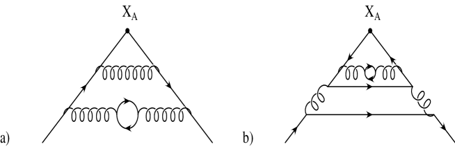
Figure 1: Examples of the two types of insertion of $X_{A}$: (a) OZI diagram; (b) Non-OZI diagram.

In order to obtain a simple alternative method for the tuning of the gluino mass to its critical value, we consider the axial WI in the “OZI approximation”. It consists in separating the insertions of the operator $X_{A}$, appearing in any correlation function, into two contributions: those arising from diagrams in which the two fermion fields of $X_{A}$ are not contracted (OZI) and those arising from diagrams in which they are (non-OZI); see Fig. 1. Note that the anomaly operator $P_{\mu\nu}\tilde{P}_{\mu\nu}$ can only arise as a counterterm to the non-OZI contributions. Thus, we may render the OZI part of $X_{A}$ finite by defining the subtraction

$$\bar{X}_{A,OZI}=\left[X_{A}+(Z_{A}^{\prime}-1)\nabla_{\mu}A_{\mu}+2\bar{m}^{\prime}P\right]_{OZI}$$ (30)

and imposing $\lim_{a\rightarrow 0}\;\bar{X}_{A,OZI}=0$. A renormalized WI can then be obtained

$$\nabla_{\mu}{\hat{A}}^{\prime}_{\mu}=2(m_{0}-{\bar{m}}^{\prime})(Z_{P}^{\prime})^{-1}{\hat{P}}^{\prime}+{\cal O}(a),$$ (31)

with ${\hat{A}}^{\prime}_{\mu}=Z^{\prime}_{A}A_{\mu}$ and $\hat{P}^{\prime}=Z^{\prime}_{P}P$. This WI is an operator relation, which holds in any OZI amplitude. Now, using eq. (31) it is easy to get the point $m_{0}=\bar{m}^{\prime}(m_{0},g_{0})$ by tuning to zero the ratio $2\rho_{OZI}$:

$$2\rho_{OZI}\equiv\frac{\nabla_{\mu}\langle{A}_{\mu}(x)P(0)\rangle|_{OZI}}{\langle P(x)P(0)\rangle|_{OZI}}=\frac{m_{0}-{\bar{m}}^{\prime}}{Z^{\prime}_{A}}.$$ (32)

However, this is only useful if $m_{0}-{\bar{m}}^{\prime}$ vanishes at the same critical point where $m_{0}-{\bar{m}}=0$, which is not at all obvious. To see how this may come about, we also consider the subtractions generated by the non-OZI part of $X_{A}$; these are

$$\bar{X}_{A,non-OZI}=\left[X_{A}-Z_{A}^{\prime\prime}\nabla_{\mu}A_{\mu}-Z_{Q}P_{\mu\nu}\tilde{P}_{\mu\nu}+2\bar{m}^{\prime\prime}P\right]_{non-OZI}.$$ (33)

The sum of OZI and non-OZI insertions must reproduce the anomalous renormalized WI (19). This implies that the OZI tuning of $m_{0}-{\bar{m}}^{\prime}$ and that of $m_{0}-{\bar{m}}$ occur at the same point $m_{cr}$, provided

$${\bar{m}}^{\prime\prime}(m_{cr},g_{0}^{2})=0.$$ (34)

This is expected to be the case for a theory with more gluino flavours, $N_{f}>1$. In such a theory, the previous reasoning holds, but in addition there is an additional non-singlet chiral symmetry, which yields the standard non-anomalous PCAC WI. The explicit breaking of this symmetry, contained in $X^{NS}_{A}$, can be subtracted through renormalization

$$\bar{X}^{NS}_{A}=X^{NS}_{A}+(Z_{A}^{\prime}-1)\nabla_{\mu}A^{NS}_{\mu}+2\bar{m}^{\prime}P^{NS},$$ (35)

where the superscript $NS$ stands for non-singlet current and operator. As usual, the renormalization condition is $\lim_{a\rightarrow 0}\bar{X}^{NS}_{A}=0$. Notice that $Z^{\prime}_{A}$ and $\bar{m}^{\prime}$ are identical to those appearing in the OZI singlet WI, eq. (30), since the insertions of $X^{NS}_{A}$ only have OZI contributions.

In the continuum limit we should recover the expected continuum WIs:

$$\nabla_{\mu}{\hat{A}}_{\mu}^{NS} = 2\hat{m}_{\lambda}{\hat{P}}^{NS},$$ (36)

$$\nabla_{\mu}{\hat{A}}_{\mu} = 2\hat{m}_{\lambda}{\hat{P}}+{\hat{Q}}.$$

Notice that, in the continuum, the renormalized gluino mass appearing in both WIs is the same. It then follows that

$$\hat{m}_{\lambda}=\frac{m_{0}-\bar{m}^{\prime}-\bar{m}^{\prime\prime}}{Z_{P}}=\frac{m_{0}-\bar{m}^{\prime}}{Z_{P}^{NS}},$$ (37)

where $\hat{P}^{NS}=Z_{P}^{NS}P^{NS}$. This implies that, at the critical point defined from eq. (32), eq. (34) is verified. If we further assume that the dependence of $\bar{m}^{\prime\prime}(m_{cr},g_{0})$ on $N_{f}$ is analytic, this result should also hold in the $N_{f}=1$ case. In this case, the point of symmetry restoration is given, up to ${\cal O}(a)$ terms, by the vanishing of $2\rho_{OZI}$; c.f. eq.(32).

The computations of the present paper have been performed in the quenched-OZI approximation. In this case, the requirement that $\bar{m}^{\prime\prime}$ be analytic in $N_{f}$ can be relaxed, since the OZI two-point correlation functions are identical to the non-singlet ones in a theory with $N_{f}=2$ (internal fermion loops, which could depend on $N_{f}$, are absent). Hence, the tuning to the zero gluino-mass limit can be done using eq. (32). Furthermore, it is believed that, in these approximations, spontaneous chiral symmetry breaking occurs because of a non-vanishing gluino condensate [6, 7]. If that is the case, the OZI pseudoscalar $\tilde{\pi}$ should become massless in the zero gluino–mass limit. The two requirements $m_{\tilde{\pi}}\rightarrow 0$ and $2\rho\rightarrow 0$ give two determinations of $m_{0}$, which should only coincide if chiral symmetry is spontaneously broken. We will see that this is confirmed numerically.

3.3 Order parameter of supersymmetry breaking

WIs can also be used to study the issue of spontaneous supersymmetry breaking, in complete analogy with the study of spontaneous breaking of the non-singlet chiral symmetry in QCD described in [12]. Consider the supersymmetric WI,

$$\langle\nabla_{\mu}{\hat{S}}_{\mu}(x)\hat{\chi}(0)\rangle=2(m_{0}-\tilde{m})Z^{-1}_{\chi}\langle{\hat{\chi}}(x)\hat{\chi}(0)\rangle+\;\delta^{4}(x)\langle{\hat{F}}(x)\rangle.$$ (38)

The operator $\hat{F}$ is the renormalized vacuum expectation value of the bare auxiliary field of the $\Phi$ supermultiplet. Thus it is the order parameter of SUSY breaking. For a non-zero gluino mass, we can integrate the previous relation over space-time and obtain

$$0=2\;(m_{0}-\tilde{m})\sum_{x}Z^{-1}_{\chi}\langle\hat{\chi}(x)\hat{\chi}(0)\rangle+\langle\hat{F}(0)\rangle.$$ (39)

The renormalized order parameter for spontaneous SUSY breaking can then be computed as

$$\langle\hat{F}(0)\rangle=-2\;\lim_{m_{0}\rightarrow m_{cr}}\;\;(m_{0}-\tilde{m})\sum_{x}Z^{-1}_{\chi}\langle\hat{\chi}(x)\hat{\chi}(0)\rangle.$$ (40)

If this expectation value does not vanish, then SUSY is spontaneously broken. In this case the WI also implies that, in the supersymmetric limit, there exists a massless fermion field which propagates in the $\langle\chi\chi\rangle$ channel. This is the Goldstone fermion of supersymmetry breaking (the goldstino). Hence, another signal of spontaneous supersymmetry breaking would be to find a massless fermion in the channel $\langle\chi(x)\chi(y)\rangle$ in the limit of zero gluino mass (where this limit is defined by using eq. (28) or eq. (29)).

4 Correlation functions

In this section we discuss the method for extracting the lowest-lying masses of the pseudoscalar, scalar and spinor particles of the supermultiplet $\Phi$ (i.e. $\tilde{\pi}$, $\tilde{\sigma}$ and $\tilde{\chi}$, respectively), in the OZI approximation.

The two-point correlation functions used to obtain the $\tilde{\pi}$ and $\tilde{\sigma}$ masses are

$$C_{PP}(t) = \sum_{\vec{x}}\langle P(\vec{x},t)P(\vec{x}_{0},t_{0})\rangle,$$

$$C_{SS}(t) = \sum_{\vec{x}}\langle S(\vec{x},t)S(\vec{x}_{0},t_{0})\rangle.$$ (41)

In order to compute $2\rho$ we need also the following correlation functions:

$$C_{AP}(t) = \sum_{\vec{x}}\langle A_{0}(\vec{x},t)P(\vec{x}_{0},t_{0})\rangle,$$

$$C_{PA}(t) = \sum_{\vec{x}}\langle P(\vec{x},t)A_{0}(\vec{x}_{0},t_{0})\rangle.$$ (42)

In the computation of all these correlations, the point ($\vec{x}_{0},t_{0}$) is held fixed at the origin. The correlations $C_{AP}$ and $C_{PA}$ are antisymmetrized, in order to enhance the signal-to-noise ratio (from now on $C_{AP}$ stands for the antisymmetrized correlation function). The quantity $2\rho$ is obtained from the ratio:

$$R(t)=\frac{\nabla_{0}C_{AP}(t)}{C_{PP}(t)}.$$ (43)

where $\nabla_{\mu}f(x)\equiv[f(x+\hat{\mu})-f(x-\hat{\mu})]/2$ is a symmetric lattice derivative.

We now express the two-point correlation functions of eqs. (41)–(43) in terms of gluino propagators. The correlation function

$$C(t)=\sum_{\vec{x}}\langle O_{1}(x)O_{2}(x_{0})\rangle$$ (44)

of two generic bilocal operators $O_{i}=\bar{\lambda}\Gamma_{i}\lambda$, with $\Gamma_{i}$ any Dirac matrix ($i=1,2$), can be written as

$$C(t)= - \sum_{\vec{x}}\langle{\rm Tr}[Q(\vec{x},t;\vec{x}_{0},t_{0};U_{\mu})\Gamma_{2}Q(\vec{x}_{0},t_{0};\vec{x},t;U_{\mu})\Gamma_{1}]\rangle$$

$$+ \sum_{\vec{x}}\langle{\rm Tr}[Q(\vec{x},t;\vec{x},t;U_{\mu})\Gamma_{1}]{\rm Tr}[Q(\vec{x}_{0},t_{0};\vec{x}_{0},t_{0};U_{\mu})\Gamma_{2}]\rangle$$

$$+ \sum_{\vec{x}}\langle{\rm Tr}[Q(\vec{x},t;\vec{x}_{0},t_{0};U_{\mu})\Gamma_{2}Q(\vec{x}_{0},t_{0};\vec{x},t;U_{\mu})C\Gamma_{1}^{T}C]\rangle,$$

where $Q(\vec{x},t;\vec{0},0;U_{\mu})=\Delta^{-1}(\vec{x},t;\vec{0},0;U_{\mu})$ is the fermion propagator, computed on a single background field configuration (i.e. the inverse of the fermion matrix). The first two terms of the above expression are the familiar one- and two-boundary quark diagrams which also appear in the Dirac fermion formulation. The third term arises from the extra contractions characteristic of Majorana fermions; see also comments after eq. (11). It is also a one-boundary quark diagram. For the cases of interest (i.e. eqs. (41)–(43)), we have that $C\Gamma_{1}^{T}C=-\Gamma_{1}$, and the first and third terms are equal. In the present work we are interested in the OZI approximation of the above expression, for which the second term does not contribute. In other words, we compute only one-boundary diagrams.

For the $\tilde{\chi}$ mass, we use the two-point correlation function

$$[C_{\tilde{\chi}}(t)]_{\alpha\beta} = \sum_{\vec{x},\vec{x}_{0}}\langle\chi_{\alpha}(\vec{x},t)\bar{\chi}_{\beta}(\vec{x}_{0},t_{0})\rangle$$ (46)

$$= \frac{1}{4}\langle\left(\sigma_{\mu\nu}\right)_{\alpha\alpha^{\prime}}P_{\mu\nu}^{a}(\vec{x},t)Q^{ab}_{\alpha^{\prime}\beta^{\prime}}(\vec{x},t;\vec{x}_{0},t_{0};U_{\mu})P_{\rho\sigma}^{b}(\vec{x}_{0},t_{0})\left(\sigma_{\rho\sigma}\right)_{\beta^{\prime}\beta}\rangle.$$

This correlation remains unchanged in the OZI approximation, as it only has one valence gluino line. For $C_{\tilde{\chi}}(t)$, we keep $t_{0}$ at the origin and vary $\vec{x}_{0}$ over the whole time-slice $t_{0}$. This is obtained in the simulations by solving numerically the equation

$$\Delta^{aa^{\prime}}_{\alpha\beta^{\prime}}(\vec{x},t;\vec{x}^{\prime},t^{\prime})\Sigma^{a^{\prime}}_{\beta^{\prime}\beta}(\vec{x}^{\prime},t^{\prime};\vec{x}_{0},t_{0})=\delta^{3}_{\vec{x},\vec{x}_{0}}\delta_{t,t_{0}}P_{\mu\nu}^{a}(\vec{x},t)\left(\sigma_{\mu\nu}\right)_{\alpha\beta}.$$ (47)

The solution of the above is

$$\Sigma^{a}_{\alpha\beta}(\vec{x},t;\vec{x}_{0},t_{0})=Q^{aa^{\prime}}_{\alpha\alpha^{\prime}}(\vec{x},t;\vec{x}_{0},t_{0};U_{\mu})P_{\mu\nu}^{a^{\prime}}(\vec{x}_{0},t_{0})\left(\sigma_{\mu\nu}\right)_{\alpha^{\prime}\beta},$$ (48)

as can be verified by back substitution. Once $\Sigma$ has been obtained numerically by inverting eq. (47), the correlation $C_{\tilde{\chi}}$ can be easily computed. By using various properties (parity, time reversal, etc.) we show in Appendix B that the correlation function has the form

$$[C_{\tilde{\chi}}(t)]_{\alpha\beta}=C_{1}(t)\delta_{\alpha\beta}+C_{2}(t)\gamma^{0}_{\alpha\beta}.$$ (49)

We recall that the local operator $\chi_{\alpha}(x)$ also extends in the time direction, since it contains the field strength tensor $P^{a}_{\mu\nu}$. In order to eliminate the contact terms arising from adjacent time-slices, we have also considered the operator that has only the spatial component of the field strength, defined as follows:

$$\chi^{S}_{\alpha}(x)=\frac{1}{2}F^{a}_{ij}(x)\left(\sigma_{ij}\right)_{\alpha\beta}\lambda^{a}_{\beta},$$ (50)

where $i,j=1,2,3$. Its two-point correlation function is given by:

$$[C^{S}_{\tilde{\chi}}(t)]_{\alpha\beta} = \sum_{\vec{x},\vec{x}_{0}}\langle\chi^{S}_{\alpha}(\vec{x},t)\bar{\chi}^{S}_{\beta}(\vec{x}_{0},t_{0})\rangle$$ (51)

$$= \frac{1}{4}\left(\sigma_{ij}\right)_{\alpha\alpha^{\prime}}P_{ij}^{a}(\vec{x},t)Q^{ab}_{\alpha^{\prime}\beta^{\prime}}(\vec{x},t;\vec{x}_{0},t_{0})P_{kl}^{b}(\vec{x}_{0},t_{0})\left(\sigma_{kl}\right)_{\beta^{\prime}\beta},$$

where $i,j,k,l=1,2,3$.

The $\tilde{\pi}$, $\tilde{\sigma}$ and $\tilde{\chi}$ masses are extracted from the asymptotic behaviour of the corresponding correlation functions at large time separations. In principle, both form factors of eq. (49) should decay exponentially in time with the same mass. Hence, we can obtain in principle two independent measurements of the $\tilde{\chi}$ mass.

5 Particle masses

We have performed simulations at $\beta=2.6$. The lattice volume is $V=16^{3}\times 32$. We have generated quenched configurations, separated by 400 thermalizing sweeps, with a standard hybrid heat-bath algorithm. We have measured 950 gluino propagators (the measurement has been made every 30 sweeps) at four values of the hopping parameter: $K=0.174,\,0.178,\,0.182,\,0.184$. In [15], simulations performed at $\beta=2.3$ gave too large a value for the $\tilde{\sigma}$ (greater than 1.5 in lattice units). We have opted for a larger $\beta$ value, hoping to keep all masses smaller than 1 (in lattice units), by reducing the UV cutoff $a$. Statistical errors have been obtained with the jacknife method, by discarding 10 configurations at a time. Unfortunately the time extension of the lattice seems a little too short to isolate the lowest-lying state in the $\tilde{\pi}$ channel and two-exponential fits are needed in this case. This increases the statistical error in this channel.

5.1 The $\tilde{\pi}$ particle

We isolate the lowest-lying mass of the correlation function $C_{PP}(t)$ by fitting it with the function

$$C_{PP}(t)=\frac{Z_{1}}{2m}\exp(-mt)\left[1+Z_{2}\exp(-\Delta mt)\right]+\left(t\rightarrow T-t\right).$$ (52)

We have used this two-state fit in order to estimate the lowest mass, by fitting in time interval $t_{i}\leq t\leq T/2-1$, where $T=32$ is the time extension of the lattice. In table 1 we show the results of our two-state fits at the different values of the gluino mass as a function of the initial time $t_{i}$.

$K$	$t_{i}=6$	$t_{i}=7$	$t_{i}=8$	$t_{i}=9$	$t_{i}=10$
$0.174$	$0.869(2)$	$0.867(2)$	$0.864(5)$	$0.855(6)$	$0.860(7)$
$0.174$	$-$	$-$	$0.876(1)$	$-$	$-$
$0.178$	$0.713(2)$	$0.711(2)$	$0.707(5)$	$0.698(8)$	$0.703(11)$
$0.178$	$-$	$-$	$0.720(1)$	$-$	$-$
$0.182$	$0.536(2)$	$0.534(3)$	$0.531(4)$	$0.526(11)$	$0.528(11)$
$0.182$	$-$	$-$	$0.543(1)$	$-$	$-$
$0.184$	$0.433(2)$	$0.432(3)$	$0.430(4)$	$0.428(7)$	$0.426(9)$
$0.184$	$-$	$-$	$0.441(1)$	$-$	$-$

Table 1: The mass of $\tilde{\pi}$ as a function of initial fitting time. For each $K$ value, data at the top (for $6\leq t_{i}\leq 10)$ are the results from two-mass fits, whereas the data at the bottom of the $t_{i}=8$ column are those from one-mass fits.

We note that the two-mass fit results decrease with increasing $t_{i}$ in the interval $6\leq t_{i}\leq 8$. This probably signals the weak residual presence of a higher mass state. Since, however, from $t_{i}=8$ onwards, the values are fluctuating within their error, the isolation of two low-lying states is achieved. As $t_{i}$ increases, so does the statistical error. We take as the best estimates of the $\tilde{\pi}$ mass the results of $t_{i}=8$. As a further test, we did a one-state fit, also shown in table 1, in the interval $8\leq t\leq 16$. The results are systematically higher than the ones obtained at the same interval with the two-mass fit. This further justifies the necessity for the latter fit.

5.2 The $\tilde{\sigma}$ particle

The $\tilde{\sigma}$ particle is noisier than the $\tilde{\pi}$. In table 2 we show the results of the following one-state fit for this correlation:

$$C_{SS}(t)=Z_{0}+\frac{Z_{1}}{2m}\left[\exp\left(m(t-T)\right)+\exp(-mt)\right].$$ (53)

We take as our best estimates the masses from $t_{i}=10$. In all cases, the constant $Z_{0}$ was compatible with zero (and orders of magnitude smaller than $Z_{1}$). This is hardly surprising, since, working in the OZI approximation, we are only measuring the contribution of the one-boundary diagram to the above correlation function. This contribution is equal to the two-point correlation function of the corresponding non-singlet scalar operator $S^{NS}(x)$, for which $Z_{0}=0$.

In fig. 2 we present the effective masses for the $\tilde{\pi}$ and $\tilde{\sigma}$ as a function of $t$, compared with the results of eqs. (52) and (53) at $K=0.182$. It is clear that the curves fit the data well. However, lattices with larger time extensions are needed for the effective mass of $\tilde{\pi}$ to reach a plateau. In the case of the $\tilde{\sigma}$, the effective mass plot displays a plateau. The straightforward measurement of the $\tilde{\sigma}$ mass in our case must be contrasted to the situation in quenched QCD, where the signal for the scalar particle $\sigma$ is extremely noisy.

$K$	$t_{i}=7$	$t_{i}=8$	$t_{i}=9$	$t_{i}=10$	$t_{i}=11$
$0.174$	$1.13(1)$	$1.11(2)$	$1.10(2)$	$1.09(2)$	$1.08(3)$
$0.178$	$0.99(1)$	$0.97(2)$	$0.95(2)$	$0.95(3)$	$0.93(3)$
$0.182$	$0.83(2)$	$0.82(2)$	$0.81(3)$	$0.81(4)$	$0.80(5)$
$0.184$	$0.75(3)$	$0.74(3)$	$0.74(5)$	$0.76(6)$	$0.76(9)$

Table 2: The mass of $\tilde{\sigma}$ as a function of initial fitting time.

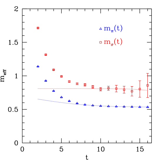
Figure 2: Effective masses for $\tilde{\pi}$ (below) and $\tilde{\sigma}$ (above) as a function of time at $K=0.182$, compared with results of the fits (dotted lines).

5.3 The $2\rho$ correlation

The ratio $R(t)$, which gives the estimate of $2\rho$, is shown in fig. 3 (for $K=0.178$). A plateau sets in at fairly early times. We perform a weighted average of the results in the time interval $9\leq t\leq 14$. The $2\rho$ estimates thus obtained are shown in table 3.

$K$	$0.174$	$0.178$	$0.182$	$0.184$
$2\rho$	$0.379(2)$	$0.254(2)$	$0.145(1)$	$0.096(1)$

Table 3: The values of $2\rho$ as a function of $K$.

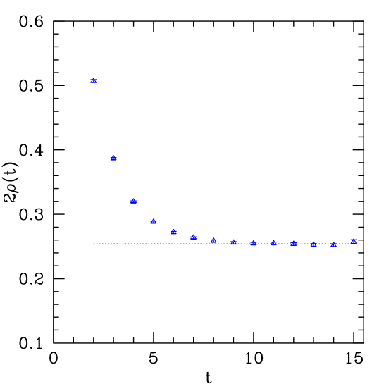
Figure 3: $R(t)$ as a function of time at $K=0.178$. The dotted line is its average value in the time interval 9-14.

5.4 The $\tilde{\chi}$ particle

We have obtained the effective mass of $\tilde{\chi}$ from the spatial correlation function of eq. (51). We used all the properties of $C_{\tilde{\chi}}^{S}(t)$ under the discrete symmetries (explained in full detail in Appendix B), in order to isolate the two independent components of the correlation, namely $C_{1}(t)$ and $C_{2}(t)$. No effective mass can be obtained naively from either $C_{1}(t)$ or $C_{2}(t)$, owing to large statistical fluctuations. In order to improve the signal-to-noise ratio, we implemented the smearing à la APE [16], which is widely adopted in glueball spectroscopy. The value of the smearing optimization parameter $\epsilon$ of [16] is fixed at $\epsilon=0.5$. We have obtained results with two smearing steps, namely $n_{s}=4$ and $n_{s}=8$. In fig. 4 we show the effective mass extracted from $C_{1}(t)$ and $C_{2}(t)$ at $K=0.174$ as a function of time ($m_{1}$ and $m_{2}$ respectively), with $n_{s}=4$ and $n_{s}=8$. The results obtained with $n_{s}=4$ show a plateau at small times; this is reminiscent of the results for the glueball masses, obtained with the same method. The results with $n_{s}=8$ have somewhat smaller statistical errors up to times $t=5$, but the values fluctuate more as a function of $t$. We plan to study the optimization of the number of smearing steps in a future simulation. Since the signal obtained from $C_{2}(t)$ is cleaner than that obtained from $C_{1}(t)$, in this paper we use the former correlation function in order to extract the $\tilde{\chi}$ mass. We take as our best estimates of the $\tilde{\chi}$ mass the results for $m_{2}$ in the interval $3\leq t\leq 5$, for $n_{s}=4$, shown in table 4.

$K$	$0.174$	$0.178$	$0.182$	$0.184$
$m_{\tilde{\chi}}$	$0.93(12)$	$0.84(11)$	$0.73(10)$	$0.66(9)$

Table 4: The values of the $\tilde{\chi}$ effective mass as a function of $K$.

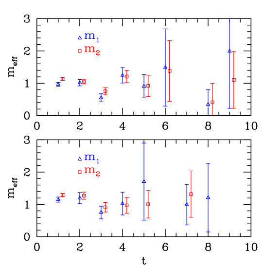
Figure 4: Effective mass of $C_{1}(t)$ and $C_{2}(t)$ at $K=0.174$ as a function of time ($m_{1}$ and $m_{2}$ respectively in the text), with $n_{s}=4$ (below) and $n_{s}=8$ (above).

6 The chiral limit

As explained in section 3, in the quenched OZI approximation, chiral symmetry is not broken by the anomaly, but it is expected to be broken spontaneously [6]. If this is the case, there are two numerically independent determinations of the critical $m_{0}(K_{c})$ at which the gluino mass vanishes. The first one is obtained upon fitting the $\tilde{\pi}$ mass as a function of the hopping parameter according to the standard PCAC relation:

$$m_{\tilde{\pi}}^{2}=A\left(\frac{1}{K}-\frac{1}{K_{c}}\right).$$ (54)

By using this relation we find the chiral limit at

$$K_{c}=0.18752(9)$$ (55)

(with one-mass fits, we obtain $K_{c}=0.18759(2)$). The second possibility is to extract $K_{c}$ from the relation between two-point correlation functions derived from the WI (32) in this approximation, which implies the vanishing of $2\rho$. Extrapolating linearly $2\rho$ in $1/K$ we obtain

$$K_{c}=0.18762(4),$$ (56)

which is compatible with the previous estimate. The behaviour of the OZI component of $\tilde{\pi}$ is thus similar to that of the $\pi$ particle in QCD, and consistent with the expectation of spontaneous chiral symmetry breaking. A discrepancy in the two estimates of $K_{c}$ would imply, either that chiral symmetry is not broken (in which case the $\tilde{\pi}$ does not need to be massless for zero gluino mass, while the WI still has to be satisfied) or, more probably, the presence of large ${\cal O}(a)$ discretization errors in the correlation functions. We see that none of these possibilities occur.

In order to obtain the masses of $\tilde{\chi}$ and $\tilde{\sigma}$ at $K_{c}$, we have performed a linear extrapolation in $1/K$ (from the results of the fit for $\tilde{\sigma}$ and from the effective mass for $\tilde{\chi}$). The results are shown in fig. 5.

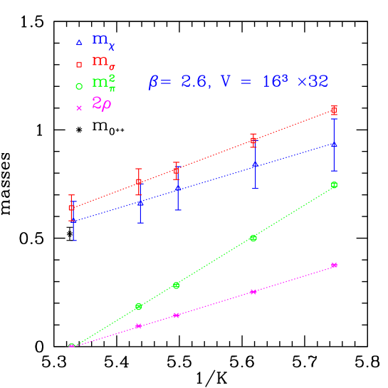
Figure 5: Masses of $\tilde{\pi},\,\tilde{\sigma},\,\tilde{\chi}$ and $2\rho$ as a function of $1/K$ (the mass of $\tilde{\pi}$ is squared). The extrapolation at $K_{c}$ is also shown (curves). The value of the $0^{++}$ glueball mass at $\beta=2.6$ is also included.

It is clear that $\tilde{\sigma}$ and $\tilde{\chi}$ do not vanish at $K_{c}$. This demonstrates that the model has QCD-like chiral behaviour, in accordance with the expectations of refs. [6, 10]. The non-vanishing of $\tilde{\sigma}$ at $K_{c}$ had already been seen in [15], at $\beta=2.3$. A comparison with [15] is possible through the ratio of the $\tilde{\sigma}$ mass to the lowest glueball mass ($0^{++}$), which has been measured for both $\beta=2.3$ and $\beta=2.6$ in [17]. The result is $\frac{m_{\tilde{\sigma}}}{m_{0^{++}}}=1.23(16)$ at $\beta=2.6$ and $1.35(16)$ at $\beta=2.3$. The two results are in fair agreement.

The dependence of the scalar and fermion masses on the gluino mass is compatible with linearity. This is expected to be the case in the unquenched theory, where the splittings in the multiplet have been computed to lowest order in the gluino mass [9]:

$$m_{\tilde{\pi}} = C+\frac{5}{6}C^{\prime}m_{\lambda},$$

$$m_{\tilde{\sigma}} = C+\frac{7}{6}C^{\prime}m_{\lambda},$$ (57)

$$m_{\tilde{\chi}} = C+C^{\prime}m_{\lambda}.$$

$C$ and $C^{\prime}$ are constants that in general depend on the renormalization scheme . We can compare the ratio of the slopes with the theoretical prediction $\Delta_{th}=1.17$. We find

$$\Delta=\frac{dm_{\tilde{\sigma}}}{dm_{\tilde{\chi}}}=1.3(5).$$ (58)

Although the error in the slope ratio is quite large, the agreement is encouraging. Moreover, the masses of $\tilde{\sigma}$ and $\tilde{\chi}$ appear to be degenerate at $K_{c}$. Of course, this does not have to be the case in the quenched-OZI approximation. Nevertheless, the mass of the $\tilde{\pi}$ particle is expected to change dramatically because of the anomaly, whereas there are no reasons to expect a dramatic change of the $\tilde{\sigma}$ and $\tilde{\chi}$ masses when the OZI and quenched approximations are relaxed. In fig. 5 the $0^{++}$ glueball mass at $\beta=2.6$ is also included. We recall that this particle represents an auxiliary field in the $\Phi$ supermultiplet, and it should be degenerate in mass with the other particles belonging to $\Phi$ in the supersymmetric limit. Its mass appears to be compatible with the extrapolated $\tilde{\chi}$ mass and $2\sigma$ below the $\tilde{\sigma}$ mass. This small discrepancy could of course be due to the effect of the OZI and/or quenched approximations on the $\tilde{\sigma}$ mass (in particular, notice that the OZI approximation only affects the $\tilde{\sigma}$ correlation function, but neither $\tilde{\chi}$ nor the glueball).

7 Conclusions

We have measured the low-lying spectrum of $SU(2)$ with one flavour of adjoint matter. This is the matter content of supersymmetric $SU(2)$. Our quenched simulation, although not yet supersymmetric, is a first step towards the understanding of the fine-tuning to the zero gluino–mass limit, which is necessary in the lattice formulation of $N=1$ supersymmetry with Wilson fermions. We have used the chiral WI to restore this limit in this work and discussed how this can also be done in the full theory.

The numerical results on the spectrum are quite encouraging. In the full theory the theoretical expectation is that SUSY is not broken spontaneously and the low-lying states are the components of a composite chiral superfield, i.e. one complex spin zero particle and its fermionic partner. Of these fields, only the imaginary part of the scalar field gets its mass from fermion loops, through the chiral anomaly. The other states are not expected to change very much when the quenched approximation is relaxed. In fact, we have found that these states are approximately degenerate at zero gluino mass, already in the quenched approximation. This could be a first signal of supersymmetry restoration at zero gluino mass on the lattice. Finally, the vanishing of the $\tilde{\pi}$ mass at the critical point is an indication of spontaneous chiral symmetry breaking, while the finite $\tilde{\chi}$ mass supports the theoretical expectation that SUSY is not spontaneously broken (although this result must be confirmed in the framework of unquenched simulations).

Acknowledgements

We thank M.B. Gavela, K. Jansen, I. Montvay, G.C. Rossi, R. Sommer, M. Testa and G. Veneziano for encouragement and/or many helpful discussions. We also thank G. Martinelli and the Rome-I lattice group for providing the computing resources that have made this work possible.

Appendix A Notation and conventions

Here we list our conventions. The number of colours is $N_{c}$ (in this work $N_{c}=2$). The number of flavours is $N_{f}$ (in this work $N_{f}=1$). Latin lower-case indices (of the form $a,b,\ldots=1,\ldots,N_{c}^{2}-1$) stand for colour in the adjoint representation. Latin upper-case indices stand for colour in the fundamental representation ($A,B,\ldots=1,\ldots,N_{c}$). Greek lower case indices from the beginning of the alphabet stand for spin ($\alpha,\beta,\ldots=1,\ldots,4$) and those from the middle of the alphabet ($\mu,\nu,\ldots=0,\ldots,3$) denote Lorentz space-time components (in Euclidean space-time). Latin lower-case indices (of the form $i,j,k,l=1,2,3$) denote Lorentz spatial components.

The gauge field is thus $U^{AB}_{\mu}(x)$, the fermion field is $\lambda_{\alpha}^{a}(x)$, the field-strength tensor is $F_{\mu\nu}^{a}(x)$, etc. It is also customary to write $\lambda_{\alpha}(x)=\lambda_{\alpha}^{a}(x)T^{a}$, $F_{\mu\nu}(x)=F_{\mu\nu}^{a}(x)T^{a}$, with the colour indices in the fundamental representation (e.g. $\lambda_{\alpha}^{AB}$, $T^{a}_{AB}$ etc.) supressed. $T^{a}$ are the group generators, normalized as follows:

$${\rm Tr}[T^{a}T^{b}]=\frac{1}{2}\delta^{ab}.$$ (59)

For $N_{c}=2$, these are the standard Pauli matrices $T^{a}=\sigma^{a}/2$.

The Dirac matrices are in the Weyl representation in Euclidean space-time. In terms of the three Pauli spin matrices and the unit $2\times 2$ matrix $I$, they are given by

$$\begin{array}[]{c}\gamma_{0}\end{array}=\left(\begin{array}[]{rr}0&I\\ I&0\end{array}\right);\qquad\begin{array}[]{c}\gamma_{k}\end{array}=-i\left(\begin{array}[]{rr}0&\sigma_{k}\\ -\sigma_{k}&0\end{array}\right).$$ (60)

We also define

$$\gamma_{5} = \gamma_{1}\gamma_{2}\gamma_{3}\gamma_{0},$$

$$\sigma_{\mu\nu} = \frac{1}{2}[\gamma_{\mu},\gamma_{\nu}],$$ (61)

$$C = \gamma_{0}\gamma_{2}.$$

We often make use of the following property of the charge conjugation matrix:

$$C^{-1}=-C=C^{T}.$$ (62)

Finally, we take the sign convention $\epsilon_{0123}=1$.

Appendix B Discrete symmetries on the lattice

In the spirit of ref. [18], we list the discrete symmetry transformations of the gauge field $U_{\mu}(x)$ and the fermion fields $\lambda(x)$ and $\bar{\lambda}(x)$ in Euclidean space-time. The symmetry transformations of the lattice field tensor $P_{\mu\nu}(x)$, the operators $\chi(x)$, $\bar{\chi}(x)$ and the gauge field in the adjoint representation $V_{\mu}(x)$ are then easily derived. We also derive useful identities between the gluino propagator $Q(x;x_{0};U_{\mu})$, computed on a single background gauge-field configuration, and the one computed on the symmetry-transformed background field. The same properties are also derived for the propagator of the $\tilde{\chi}$ operator. Finally, we derive eq. (49).

Under parity ${\cal P}$ we have:

$$(\vec{x},t_{0}) \rightarrow (\vec{x}^{{\cal P}},t_{0}^{{\cal P}})=(-\vec{x},t_{0})$$

$$\psi(x) \rightarrow \psi^{{\cal P}}(x^{{\cal P}})=\gamma_{0}\psi(x)$$

$$\bar{\psi}(x) \rightarrow \bar{\psi}^{{\cal P}}(x^{{\cal P}})=\bar{\psi}(x)\gamma_{0}$$

$$U_{0}(x) \rightarrow U_{0}^{{\cal P}}(x^{{\cal P}})=U_{0}(x)$$

$$U_{k}(x) \rightarrow U_{k}^{{\cal P}}(x^{{\cal P}})=U_{-k}(x)=U^{\dagger}_{k}(x-\hat{k})$$

$$P_{0k}(x) \rightarrow P_{0k}^{{\cal P}}(x^{{\cal P}})=-P_{0k}(x)$$ (63)

$$P_{lk}(x) \rightarrow P_{lk}^{{\cal P}}(x^{{\cal P}})=P_{lk}(x)$$

$$\chi(x) \rightarrow \chi^{{\cal P}}(x^{{\cal P}})=\gamma_{0}\chi(x)$$

$$\bar{\chi}(x) \rightarrow \bar{\chi}^{{\cal P}}(x^{{\cal P}})=\bar{\chi}(x)\gamma_{0}$$

$$V_{0}(x) \rightarrow V_{0}^{{\cal P}}(x^{{\cal P}})=V_{0}(x)$$

$$V_{k}(x) \rightarrow V_{k}^{{\cal P}}(x^{{\cal P}})=V_{-k}(x)=V_{k}(x-\hat{k})$$

Under time-reversal ${\cal T}$ we have:

$$(\vec{x},t_{0}) \rightarrow (\vec{x}^{{\cal T}},t_{0}^{{\cal T}})=(\vec{x},-t_{0})$$

$$\psi(x) \rightarrow \psi^{{\cal T}}(x^{{\cal T}})=\gamma_{0}\gamma_{5}\psi(x)$$

$$\bar{\psi}(x) \rightarrow \bar{\psi}^{{\cal T}}(x^{{\cal T}})=\bar{\psi}(x)\gamma_{5}\gamma_{0}$$

$$U_{0}(x) \rightarrow U_{0}^{{\cal T}}(x^{{\cal T}})=U_{-0}(x)=U^{\dagger}_{0}(x-\hat{0})$$

$$U_{k}(x) \rightarrow U_{k}^{{\cal T}}(x^{{\cal T}})=U_{k}(x)$$

$$P_{0k}(x) \rightarrow P_{0k}^{{\cal T}}(x^{{\cal T}})=-P_{0k}(x)$$ (64)

$$P_{lk}(x) \rightarrow P_{lk}^{{\cal T}}(x^{{\cal T}})=P_{lk}(x)$$

$$\chi(x) \rightarrow \chi^{{\cal T}}(x^{{\cal T}})=\gamma_{0}\gamma_{5}\chi(x)$$

$$\bar{\chi}(x) \rightarrow \bar{\chi}^{{\cal T}}(x^{{\cal T}})=\bar{\chi}(x)\gamma_{5}\gamma_{0}$$

$$V_{0}(x) \rightarrow V_{0}^{{\cal T}}(x^{{\cal T}})=V_{-0}(x)=V_{0}(x-\hat{0})$$

$$V_{k}(x) \rightarrow V_{k}^{{\cal T}}(x^{{\cal T}})=V_{k}(x)$$

These two discrete symmetries result in the following useful properties of the gluino propagator $Q(x;y;U_{\mu})$ valid on a single gauge-field configuration:

$$Q(x;y;U_{\mu}) = \gamma_{0}Q(x^{{\cal P}};y^{{\cal P}};U_{\mu}^{{\cal P}}(x^{{\cal P}}))\gamma_{0},$$

$$Q(x;y;U_{\mu}) = \gamma_{5}\gamma_{0}Q(x^{{\cal T}};y^{{\cal T}};U_{\mu}^{{\cal T}}(x^{{\cal T}}))\gamma_{0}\gamma_{5}.$$ (65)

The above properites are identical to the ones valid for Dirac fermions. Also, the usual $\gamma_{5}$ property, valid for Dirac fermions, is also true for Majorana fermions:

$$Q(x;y;U_{\mu}) = \gamma_{5}Q(y;x;U_{\mu})^{\dagger}\gamma_{5}.$$ (66)

We also re-write eq. (13) in the form

$$Q(x;y;U_{\mu}) = C^{-1}Q(y;x;U_{\mu})^{T}C.$$ (67)

We combine eqs. (66) and (67) to obtain:

$$Q(x;y;U_{\mu}) = C^{-1}\gamma_{5}Q(x;y;U_{\mu})^{*}\gamma_{5}C.$$ (68)

The transpose superscript $T$ and the Hermitian transpose one $\dagger$ only act on spin and colour indices, i.e. the transposition in space-time is explicit.

We now turn to the two-point correlation function of the $\tilde{\chi}$ field, computed on a single background gauge-field configuration, which we denote by $[C_{\tilde{\chi}}(t;U_{\mu})]_{\alpha\beta}$. We write

$$[C_{\tilde{\chi}}(t;U_{\mu})]_{\alpha\beta}=\sum_{\vec{x},\vec{x}_{0}}[Q_{\tilde{\chi}}(\vec{x},t;\vec{x}_{0},t_{0};U_{\mu})]_{\alpha\beta}$$ (69)

in terms of a $\tilde{\chi}$-propagator $Q_{\tilde{\chi}}$:

$$[Q_{\tilde{\chi}}(\vec{x},t;\vec{x}_{0},t_{0};U_{\mu})]_{\alpha\beta}=\frac{1}{4}\sum_{\vec{x},\vec{x}_{0}}\left(\sigma_{\mu\nu}\right)_{\alpha\alpha^{\prime}}P_{\mu\nu}^{a}(\vec{x},t)Q^{ab}_{\alpha^{\prime}\beta^{\prime}}(\vec{x},t;\vec{x}_{0},t_{0};U_{\mu})P_{\rho\sigma}^{b}(\vec{x}_{0},t_{0})\left(\sigma_{\rho\sigma}\right)_{\beta^{\prime}\beta}.$$

We shall drop the spinor subscripts $\alpha$,$\beta$ from now on. All the properties (65)–(68) are also satisfied by $Q_{\tilde{\chi}}$, as can be found by using eqs. (63), (64) and (B). The ${\cal P}$ and ${\cal T}$ properties of $Q_{\tilde{\chi}}(x,x_{0};U_{\mu})$, listed in eqs. (65), imply for the correlation $C_{\tilde{\chi}}(t;U_{\mu})$:

$$C_{\tilde{\chi}}(t;U_{\mu})=\gamma_{0}C_{\tilde{\chi}}(t;U_{\mu}^{{\cal P}})\gamma_{0},\;\;\;\;C_{\tilde{\chi}}(t;U_{\mu})=\gamma_{5}\gamma_{0}C_{\tilde{\chi}}(T-t;U_{\mu}^{{\cal T}})\gamma_{0}\gamma_{5},$$ (71)

for a single gauge-field configuration with periodic boundary conditions in time. In the first of eqs. (71) we now average over field configurations and sum over all space. This we do by $\sum_{\vec{x},\vec{x}_{0}}\int{\cal D}U_{\mu}$ on the l.h.s. and $\sum_{-\vec{x},-\vec{x}_{0}}\int{\cal D}U^{{\cal P}}_{\mu}$ on the r.h.s., in order to obtain

$$C_{\tilde{\chi}}(t)=\gamma_{0}C_{\tilde{\chi}}(t)\gamma_{0}.$$ (72)

Similarly, on the second of eqs. (71) we average over field configurations, taking $\int{\cal D}U_{\mu}$ on the l.h.s. and $\int{\cal D}U^{{\cal T}}_{\mu}$ on the r.h.s., in order to obtain

$$C_{\tilde{\chi}}(t)=\gamma_{5}\gamma_{0}C_{\tilde{\chi}}(T-t)\gamma_{0}\gamma_{5}.$$ (73)

The $\gamma_{5}$ property of eq. (66), combined with translational invariance of the propagator implies that

$$C_{\tilde{\chi}}(t)=\gamma_{5}C_{\tilde{\chi}}(T-t)^{\dagger}\gamma_{5},$$ (74)

whereas from eq. (67) and translational invariance we obtain

$$C_{\tilde{\chi}}(t)=-CC_{\tilde{\chi}}(T-t)^{T}C.$$ (75)

Finally, combining eq. (73) with (74), and (74) with (75), we obtain

$$C_{\tilde{\chi}}(t)=\gamma_{0}C_{\tilde{\chi}}^{\dagger}(t)\gamma_{0},\;\;\;\;C_{\tilde{\chi}}(t)=-C\gamma_{5}C_{\tilde{\chi}}^{*}(t)\gamma_{5}C.$$ (76)

Now, let us consider the most general form of the correlation function $C_{\tilde{\chi}}$ as a superposition of Dirac matrices:

$$C_{\tilde{\chi}}(t)=\sum_{i}C_{i}(t)\Gamma_{i},$$ (77)

with $\Gamma_{i}=I,\gamma_{5},\gamma_{\mu},\gamma_{\mu}\gamma_{5},i\sigma_{\mu\nu}$. Using eqs. (72) and (76), we reduce this expression to

$$C_{\tilde{\chi}}(t)=C_{1}(t)I+C_{2}(t)\gamma_{0}.$$ (78)

Moreover, from eq. (73) we derive that

$$C_{1}(t) = C_{1}(T-t),$$

$$C_{2}(t) = -C_{2}(T-t),$$ (79)

which, combined with eq. (74), yields that $C_{1}(t)$ and $C_{2}(t)$ are real.

By performing analogous manipulations, it is easy to obtain the same results for the “spatial” correlation $C_{\tilde{\chi}}^{S}(t)$.

Appendix C Supersymmetric Ward identity

The supersymmetric lattice transformations for the gluino fields are:

$$\left\{\begin{array}[]{lll}\delta_{\epsilon}\lambda(x)&=&-\frac{1}{2}\sigma_{\mu\nu}P_{\mu\nu}\epsilon\\ \\ \delta_{\epsilon}\bar{\lambda}(x)&=&+\frac{1}{2}\bar{\epsilon}\sigma_{\mu\nu}P_{\mu\nu}\end{array}\right.$$ (80)

where $P_{\mu\nu}(x)$, defined in eq. (15), has dimension 2. The supersymmetric transformations of the link variables are:

$$\left\{\begin{array}[]{lll}\delta_{\epsilon}U_{\mu}(x)&=&+iag\bar{\epsilon}\gamma_{\mu}\lambda(x)U_{\mu}(x)\\ \\ \delta_{\epsilon}U^{\dagger}_{\mu}(x)&=&-iagU^{\dagger}_{\mu}(x)\bar{\epsilon}\gamma_{\mu}\lambda(x)\end{array}\right.$$ (81)

In eqs. (80) and (81), $\epsilon$ is an infinitesimal fermionic parameter of dimension $-1/2$. These transformations commute with the gauge transformations and give, in the continuum limit, the continuum SUSY transformation for the vector supermultiplet.

The supersymmetric WI is:

$$\nabla_{\mu}S_{\mu}(x)=m_{0}\sigma_{\rho\sigma}P^{a}_{\rho\sigma}(x)\lambda^{a}(x)+X_{S}(x).$$ (82)

The supersymmetric current $S_{\mu}(x)$ is a dimension 7/2 operator, defined as

$$S_{\mu}(x)=-\sigma_{\rho\sigma}\gamma_{\mu}P^{a}_{\rho\sigma}(x)V^{ab}_{\mu}(x)\lambda^{b}(x+\mu).$$ (83)

In the limit $a\to 0$ it reduces to the continuum supersymmetric current.

The operator $X_{S}(x)$ is given by

$$X_{S}(x) = \frac{1}{a}\sigma_{\alpha\beta}(\gamma_{\mu}+r)\left[P^{a}_{\alpha\beta}(x)\lambda^{a}(x)-\frac{1}{2}P^{a}_{\alpha\beta}(x)V^{ab}_{\mu}(x)\lambda^{b}(x+\mu)\right.$$

$$-\left.\frac{1}{2}\lambda^{a}(x-\mu)V^{ab}_{\mu}(x-\mu)P^{b}_{\alpha\beta}(x)\right]$$

$$+ \frac{1}{a}\gamma_{\nu}\gamma_{5}\left[\lambda^{a}(x)\tilde{P}^{a}_{\mu\nu}(x)-\tilde{P}^{a}_{\mu\nu}(x-\mu)V^{ab}_{\mu}(x-\mu)\lambda^{b}(x)\right]$$

$$- g\gamma_{\mu}\lambda^{b}(x)\left[\bar{\lambda}^{a}(x)(\gamma_{\mu}-r)f_{abd}V^{dc}_{\mu}(x)\lambda^{c}(x+\mu)\right],$$

where $f_{abc}$ is the structure constant of $SU(2)$. In the naive continuum limit, $X_{S}$ is proportional to the lattice spacing times a dimension 11/2 composite operator. $X_{S}$ does not contain only terms proportional to $r$. This is because supersymmetry is broken by both the Wilson term and the explicit Lorentz group breaking (due to the finiteness of the lattice spacing). The operator $X_{S}(x)$ is irrelevant at tree level, but divergent at one loop, since it mixes with operators of dimension 11/2 or less under renormalization [10].

References

- [1] For a review on the subject, see:D. Amati et al., Phys. Rep. 162 (1988) 169; K. Intriligator and N. Seiberg, Nucl. Phys. B (Proc. Suppl.) 45 (1996) 1 and references therein.
- [2] N. Seiberg and E. Witten, Nucl. Phys. B426 (1994) 19; N. Seiberg, Phys. Rev. D49 (1994) 6857; Nucl. Phys. B435 (1995) 129.
-
[3]
O. Aharony, J. Sonnenschein, M. Peskin and S. Yankielowicz,
Phys. Rev. D52 (1995) 6157 ;
E. D’Hoker, Y. Mimura and N. Sakai, Phys. Rev. D54 (1996) 7724;
K. Konishi, Phys. Lett. B392 (1997) 101;
N. Evans, S. Hsu, M. Schwetz and S. Selipsky, Nucl. Phys. B456 (1995) 205;
N. Evans, S. Hsu and M. Schwetz, Phys. Lett. B355 (1995) 475; Nucl. Phys. B484 (1997) 124; hep-th/9703197;
L. Alvarez-Gaumé, J. Distler, C. Kounnas and M. Mariño, Int. J. Mod. Phys. A11 (1996) 4745; L. Alvarez-Gaumé and M. Mariño, Int. J. Mod. Phys. A12 (1997) 975; L. Alvarez-Gaumé, M. Mariño and F. Zamora, hep-th/9703072; hep-th/9707017. - [4] I. Montvay, Nucl. Phys. B466 (1996) 259.
- [5] A. Donini and M. Guagnelli, Phys. Lett. B383 (1996) 301.
- [6] G. Veneziano and S. Yankielowicz, Phys. Lett. B113 (1982) 231.
- [7] V.A. Novikov et al., Nucl. Phys. B229(1983)394.
- [8] E. Witten, Nucl. Phys. B202(1982)253.
- [9] A. Masiero and G. Veneziano, Nucl. Phys. B249 (1985) 593; N. Evans, S. D. Hsu and M. Schwetz, hep-th/9707260.
- [10] G. Curci and G. Veneziano, Nucl. Phys. B292 (1987) 555.
- [11] A. Donini, M. Guagnelli, P. Hernandez and A. Vladikas, talk presented at the Lattice ’97 Conference, Edinburgh, hep-lat/9708006.
- [12] L. H. Karsten and J. Smit, Nucl. Phys. B183 (1981) 103; M. Bochicchio et al., Nucl. Phys. B262 (1985) 331.
- [13] J. Smit and J. Vink, Nucl. Phys. B298 (1988) 557; C. Ungarelli, Int. J. Mod. Phys. A10 (1995) 2269.
- [14] M. Crisafulli, V. Lubicz, A. Vladikas, hep-lat/9707025.
- [15] G. Koutsoubas and I. Montvay, Phys. Lett. B398 (1997) 130.
- [16] APE collaboration, M. Albanese et al., Phys. Lett. B192 (1987) 163.
- [17] C. Michael and M. Teper, Phys. Lett. B199 (1987) 95.
- [18] C. Bernard, in “From Actions to Answers”, eds. T. DeGrand and D. Toussaint, Proceedings of the “1989 Theoretical Advanced Study Institute in Elementary Particle Physics”, University of Colorado, Boulder, USA (World Scientific, Singapore, 1990).